Totality for Mixed Inductive and Coinductive Types
Pierre Hyvernat (LAMA)

TL;DR
This paper presents a totality checker for a language with nested inductive and coinductive types, using game semantics and size-change principles to ensure recursive functions are well-behaved, aiding proof assistant reliability.
Contribution
It introduces a novel totality checker for mixed inductive and coinductive types based on game semantics and size-change analysis, with a prototype implementation.
Findings
Prototype implementation demonstrates practical effectiveness.
Game semantics approach aids in verifying totality.
Size-change principle helps ensure recursive function correctness.
Abstract
This paper introduces an ML / Haskell like programming language with nested inductive and coinductive algebraic datatypes called \chariot. Functions are defined by arbitrary recursive definitions and can thus lead to non-termination and other ``bad'' behavior. \chariot comes with a totality checker that tags possibly ill-behaved definitions. Such a totality checker is mandatory in the context of proof assistants based on type theory like Agda. Proving correctness of this checker is far from trivial and relies on - an interpretation of types as parity games, - an interpretation of correct values as winning strategies for those games, - the Lee, Jones and Ben Amram's size-change principle, used to check that the strategies induced by recursive definitions are winning. This paper develops the first two points, the last step being the subject of an upcoming paper. A prototype has been…
Click any figure to enlarge with its caption.
 Figure 0
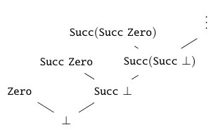 Figure 1
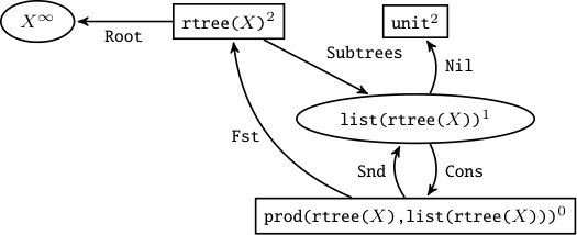 Figure 10
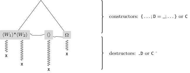 Figure 11
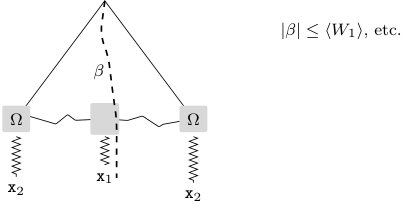 Figure 12
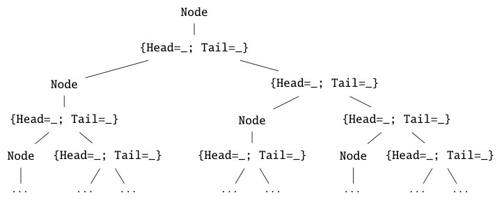 Figure 2
 Figure 3
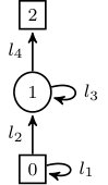 Figure 4
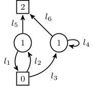 Figure 5
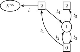 Figure 6
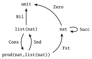 Figure 7
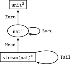 Figure 8
 Figure 9
Peer Reviews
No public reviews on file for this paper yet. If you reviewed it on a platform where reviews are public (OpenReview, ICLR, NeurIPS, ICML), you can paste yours below so the community can read it here.
Videos
No videos yet. Explain this paper in a talk, walkthrough, or lecture? Add one.
Taxonomy
TopicsLogic, programming, and type systems · Computability, Logic, AI Algorithms · Logic, Reasoning, and Knowledge
Totality for Mixed Inductive and Coinductive types
Pierre Hyvernat
Université Savoie Mont Blanc, CNRS, LAMA, 73000 Chambéry, France.
[email protected] http://lama.univ-savoie.fr/~hyvernat/
Abstract.
This paper introduces an ML / Haskell like programming language with nested inductive and coinductive algebraic datatypes called chariot. Functions are defined by arbitrary recursive definitions and can thus lead to non-termination and other “bad” behaviour. chariot comes with a totality checker that tags such bad definitions. Such a totality checker is mandatory in the context of proof assistants based on type theory like Agda.
Proving correctness of this checker is far from trivial, and relies on
- (1)
an interpretation of types as parity games due to L. Santocanale, 2. (2)
an interpretation of definitions as strategies for those games, 3. (3)
the Lee, Jones and Ben Amram’s size-change principle, used to check that those strategies are “total”.
This paper develops the first two points, the last step being the subject of an upcoming paper.
A prototype has been implemented and can be used to experiment with the resulting totality checker. It gives a practical argument in favor of this principle.
Key words and phrases:
coinductive types; nested fixed points; functional programming; recursive definitions; parity games; circular proofs
This work was partially funded by by ANR project RECIPROG, project reference ANR-21-CE48-019-01
Introduction
Inductive types (also called algebraic datatypes) are a cornerstone of typed functional programming: Haskell and Caml both rely heavily on them. One mismatch between the two languages is that Haskell is lazy while Caml is strict. A definition like
let rec nats : nat -> nat list
             = fun n -> n::(nats (n+1))
is valid but useless in Caml because the evaluation mechanism will loop trying to evaluate it completely (call-by-value evaluation), resulting in a stack overflow exception. In Haskell, because evaluation is lazy (call-by-need), such a definition isn’t unfolded until strictly necessary and asking for its third element will only unfold the definition three times. Naively, it seems that types in Caml correspond to “least fixed points” while they correspond to “greatest fixed points” in Haskell.
The aim of this paper is to introduce a language, called chariot,111All the examples will now be given using the syntax of chariot which is described in sections 1.2 and 1.5. They should be readable by anyone with a modicum of experience in functional programming. A prototype implementation in Caml is available from https://github.com/phyver/chariot for anyone wishing to experiment with it. which distinguishes between least and greatest fixed points and where the user can nest them arbitrarily to define new datatypes. To offer a familiar programming experience, definitions are not restricted and any well-typed recursive definition is allowed. In particular, it is possible to write badly behaved definitions like
val f : nat -> nat
  | f 0 = 1
  | f (n+1) = f(f n)         *– f(1) =¿ f(f(0)) =¿ f(1) =¿ …*
To guarantee that a definition is correct, two independent steps are necessary:
- (1)
Hindley-Milner type-checking [Milner] to guarantee that evaluation doesn’t provoke runtime errors, 2. (2)
a totality test to check that the definition respects the fixed points polarities involved in its type.
When no coinductive type is involved, totality amount to termination and this works is a generalization of the termination checker previously developed by the author [SCTHyvernat]. Any definition that passes this test is guaranteed to be correct but because the halting problem is undecidable, some correct definitions are rejected. In a programming context, the programmer may choose to ignore the warning if she (thinks she) knows better. In a proof-assistant context however, it cannot be ignored as non total definitions lead to inconsistencies, the most obvious example being
val magic_proof = magic_proof
which is non-terminating but belongs to all types. There are subtler examples of definitions that normalize to values but still lead to inconsistencies (c.f. example on page 1.5).
In Coq [Coq], the productivity condition for coinductive definitions is ensured by a strict syntactic condition (guardedness [Coquand93]) similar to the condition that inductive definitions need to have one structurally decreasing argument. In Agda [Agda], the user can write arbitrary recursive definitions and the productivity condition is ensured by the termination checker. Agda’s checker extends the termination checker developed by A. Abel [foetus] to deal with coinductive types, but while this is sound for simple types like streams, it is known to be unsound for nested coinductive and inductive types [ThorstenNad]. Currently, Agda’s checker is patched to deal with known counter examples like the one described in Section 1.5, but no proof of correctness is available. This paper provides a first step toward a provably correct totality checker.
Related Works
Circular proofs
The main inspiration for this work comes from ideas developed by L. Santocanale in his work on circular proofs [Luigi:muBicomplete, Luigi:CircularProofs, Luigi:parity]. Circular proofs are defined for a linear proof system and are interpreted in categories with products, coproducts and enough initial algebras / terminal coalgebras. In fine, the criterion implemented in chariot uses a strong combinatorial principle (the size-change principle) to check a sanity condition on a kind of circular proof (a program). This is strictly stronger than the initial criterion used by L. Santocanale and G. Fortier, which corresponds to the syntactical structurally decreasing / guardedness condition on recursive definitions.
However, while circular proofs were a primary inspiration, the chariot language cannot be reduced to a circular proof system. The main problem is that existing circular proof systems are linear and do not have a simple cut-elimination procedure, i.e. an evaluation mechanism. Cuts and exponentials would be needed to interpret the full chariot language and while cuts can be added [Luigi:cuts, Fortier:PHD], adding exponentials looks difficult and hasn’t been done.
More recent works in circular proof theory replace L. Santocanale’s criterion by a much stronger combinatorial condition [doumanePHD, doumane_completeness]. It involves checking that some infinite words are recognized by a parity automata, which is a decidable problem. The presence of parity automata points to a relation between this work and the present paper, but the different contexts make it all but obvious.
Size-change principle
The second idea will be developped in an upcoming paper and consists of adapting the size-change principle (SCP) from C. S. Lee, N. D. Jones and A. M. Ben-Amram [SCT] to the task of checking general totality. This problem is subtle as totality is strictly more than termination and productivity. Moreover, while the principle used to check termination of ML-like recursive definitions [SCTHyvernat] was inherently untyped, totality checking needs to be somewhat type aware. For example, in chariot, records are lazy and are used to define coinductive types. The definition
val inf = Node { Left = inf; Right = inf } *– infinite binary tree*
yields an infinite binary tree and depending on the types of Node, Fst and Snd, the definition may be correct or incorrect (c.f. page 2)!
Charity
The closest ancestor to chariot is the language charity222By the way, the name chariot was chosen as a reminder of this genealogy. [charity, charitable], developed by R. Cockett and T. Fukushima. It lets the programmer define types with arbitrary nesting of induction and coinduction. Values in these types are defined using categorical principles.
- •
Inductive types are initial algebras: defining a function from an inductive type amounts to defining an algebra for the corresponding operator.
- •
Coinductive types are terminal coalgebras: defining a function to an inductive type amount to defining a coalgebra for the corresponding operator.
It means that recursive functions can only be defined via eliminators. By construction, they are either “trivially” structurally decreasing on their argument, or “trivially” guarded. The advantage is that all functions are total by construction and the disadvantage is that the language is not Turing complete.
Guarded recursion
Another approach to checking correctness of recursive definitions is based on “guarded recursion”, initiated by H. Nakano [nakano] and later extended in several directions [birkedal, guatto]. In this approach, a new modality “later”, written “”, is introduced. The type “” gives a syntactical way to talk about terms that “will later, after some computation, have type ”. This work is quite successful and has been extended to very expressive type systems. The drawbacks are that this requires a non-standard type theory with a not quite standard denotational semantics (topos of trees). Moreover, it makes programming more difficult as it introduces new constructors for types and terms. Finally, these works only consider greatest fixed points (as in Haskell) and are thus of limited interest for systems like Agda or Coq.
Sized types
This approach extends type theory with a notion of “size” that annotate types. It has been successful and is implemented in Agda [Andreas, Andreas2]. It is possible to specify that the map function on list has type , where is the type of lists with elements of type . These extra parameters give information about recursive functions and make it easier to check termination. A drawback is that functions on sized-types must take extra size parameters. This complexity is balanced by the fact that most of them can be inferred automatically and are thus mostly the libraries’ implementors job: in many cases, sizes are invisible to the casual user. Note however that sizes only help showing termination and productivity. Developing a totality checker is orthogonal to designing an appropriate notion of size and the totality checker described in this paper can probably work hand in hand with standard size notions.
Fixed points in game semantics
An important tool in this paper is the notion of parity game. P. Clairambault [clairambault13] explored a category of games enriched with winning conditions for infinite plays. The way the winning condition is defined for least and greatest fixed points is reminiscent of L. Santocanale’s work on circular proofs and the corresponding category is cartesian closed. Because this work is done in a more complex setting and aims for generality, it seems difficult to extract a practical test for totality from it. The present paper aims for specificity and practicality by devising a totality test for the usual semantics of recursion.
SubML
C. Raffalli and R. Lepigre used the size-change principle to check correctness of recursive definitions in the language SubML [subml]. Their approach uses a powerful but non-standard type theory with many features: subtyping, polymorphism, sized-types, control operators, some kind of dependent types, etc. On the downside, it makes their type theory more difficult to compare with other approaches. Note that like in Agda or chariot, they do allow arbitrary definitions that are checked by an incomplete totality checker. One interesting point of their work is that the size-change termination is only used to check that some object (a proof tree) is well-founded: even coinductive types are justified with well-founded proofs.
Plan of the Paper
We start by introducing the language chariot and its denotational semantics in Section 1. We assume the reader is familiar with functional programming, recursive definitions and their semantics, Hindley-Milner type checking, algebraic datatypes, pattern matching, etc. The notion of totality is also given there. Briefly, it generalizes termination and productivity in a way that accounts for inductive and coinductive types. We then describe, in Section 2, a combinatorial approach to totality that comes from L. Santocanale’s work on circular proofs. This reduces checking totality of a definition to checking that the definitions gives a winning strategy in a parity game associated to the type of the definition.
The rest of the totality checker will be described in an upcoming paper [callgraphSCP].The first step will consist of developing an abstract interpretation of recursive definitions that can accommodate the size-change principle. This semantics will be both untyped and non-deterministic. The notion of call-graph, central to the implementation of the size-change principle can be defined on top of that. Applying and implementing the size-change principle follows naturally from there.
1. The Language and its Semantics
1.1. Values
Given a recursive definition, we are interested in the “healthiness” of its semantics. Such considerations take place in the realm of semantics values, and while every reader will have her favorite programming language and reduction strategy, those are mostly irrelevant to the rest of the paper.
Any finite list of recursive definitions only involves a finite number of types, with a finite number of constructors and destructors. We thus fix, once and for all, a finite set of constructor and destructor names. Because we deal with semantically infinite values, the next definition is of course coinductive. {defi} The set of values with leaves in ,…, , written is defined coinductively by the grammar
[TABLE]
where
- •
each is in one of the ,
- •
each C belongs to a finite set of constructors,
- •
each belongs to a finite set of destructors,
- •
the order of fields inside records is unimportant,
- •
can be 0.
To make the theory slightly less verbose, constructors always have a single argument. Expressivity doesn’t suffer because we can always use a tuple as argument. Of course, the implementation of chariot allows constructors of arbitrary arity.
{defi}
If the are ordered sets, the order on is generated by
- (1)
for all values , 2. (2)
if in , then in , 3. (3)
“” is contextual: if then for any value , where substitution is defined in the obvious way.
As opposed to Definition 1.1, this definition is not coinductive and reasoning about the order is usually done using simple inductive proofs.
1.2. Type Definitions
The approach described in this paper is first-order: we are only interested in the way values in datatypes are constructed and destructed. Higher order parameters are allowed in the implementation but they are ignored by the totality checker. The examples in the paper will use such higher order parameters but for simplicity’s sake, they are not formalized.333Note that can’t formally ignore higher order parameters as they can hide some recursive calls:
val app f x = f x --*non recursive
* val g x = app g x --non terminating The implementation first checks that all recursive functions are fully applied. If that is not the case, the checker aborts and gives a negative answer.
Just like in charity, types in chariot come in two flavors: those corresponding to sum types (i.e. colimits) and those corresponding to product types (i.e. limits). The syntax is itself similar to that of charity:
- •
a data comes with a list of constructors whose codomain is the type being defined,
- •
a codata comes with a list of destructors whose domain is the type being defined.
{defi}
Datatypes are introduced by the keywords “data” or “codata” and may have parameters. Types parameters are written with a quote as in Caml. The syntax is:
data (’x, ...) where | : -> (’x, ...) ... | : -> (’x, ...)
codata (’x, ...) where | : (’x, ...) -> ... | : (’x, ...) ->
where each is built from earlier types, parameters and (’x, ...). Note that type definitions are uniform in that the parameters of are the same everywhere in the definition.
Mutually recursive types are possible, but they need to be of the same polarity (all data or all codata) and all of them need to have exactly the same parameters “(’x, ...)”.
Here are some examples:
codata unit where                                      --* unit type: no destructor*

codata prod(’x,’y) where  Fst : prod(’x,’y) -> ’x                     --* pairs*
                        | Snd : prod(’x,’y) -> ’y

data nat where  Zero : unit -> nat                     --* unary natural numbers*
              | Succ : nat  -> nat

data list(’x) where  Nil  : unit               -> list(’x)        --* finite lists*
                   | Cons : prod(’x, list(’x)) -> list(’x)

codata stream(’x) where  Head : stream(’x) -> ’x             --* infinite streams*
                       | Tail : stream(’x) -> stream(’x)
Examples will sometimes use shortcuts, allowed in the implementation, and write Zero (instead of Zero{}) or Cons(x,xs) (instead of Cons{Fst=x;Snd=xs}).
Destructors act as projections, and because of the universal property of terminal coalgebras, we think about elements of a codatatype as records. This is reflected in the syntax of terms. For example, the following defines (recursively) the stream with infinitely many [math]s. (The syntax for recursive definitions will be formally given in Definition 1.5.)
val zeros : stream(nat)
  | zeros = { Head = Zero ; Tail = zeros }
Codata are going to be interpreted as coinductive types, while data are going to be inductive. The denotational semantics will reflect that, and in order to have a sound operational semantics, codata should not be fully evaluated. The easiest way to ensure that is to stop evaluation on records: evaluating “zeros” will give “{Head = ; Tail = }” where the “” are not evaluated. The copattern view [abel_copatterns] is natural here. The definition of zeros using copatterns (allowed in chariot) looks like
val zeros : stream(nat)
  | zeros.Head = Zero
  | zeros.Tail = zeros
We can interpret the clauses as a terminating rewriting system. In particular, the term zeros doesn’t reduce by itself. Because this paper is only interested in the denotational semantics of definitions, the details of the evaluation mechanism are fortunately irrelevant and the two definitions are equivalent.
We will use the following conventions:
- •
outside of actual type definitions (given using chariot’s syntax), type parameters will be written without quote: x, , …
- •
an unknown datatype will be called and an unknown codatatype will be called ,
- •
an unknown type of unspecified polarity will be called .
1.3. Semantics in Domains
There is a natural interpretation of types in the category of algebraic DCPOs where morphisms are continuous functions that are not required to preserve the least element. An algebraic DCPO is an order with the following properties:
- •
every directed set has a least upper bound (DCPO),
- •
it has a basis of compact elements (algebraic).
Unless specified otherwise, “domain” will always refer to an algebraic DCPO. Recall that any partial order can be completed to a DCPO whose compact elements are exactly the element of the partial order. This ideal completion formally adds limits of all directed sets. The following can be proved directly but is also a direct consequence of this general construction.
Lemma 1**.**
If the s are domains, then \big{(}\mathcal{V}(X_{1},\dots,X_{n}),\leq\big{)} is a domain.
Type expressions with parameters are generated by the grammar
[TABLE]
where is any domain (or set, depending on the context) called a parameter, and is the name of a datatype of arity and is the name of a codatatype of arity . A type is closed if it doesn’t contain variables. It may contain parameters though.
{defi}
The interpretation of a closed type T\big{(}\overline{X\,}\big{)} with domain parameters is defined coinductively from the following typing rules:
- (1)
\displaystyle\frac{\phantom{\big{(}}\quad{\displaystyle}\quad}{\phantom{\Big{(}}\quad{\displaystyle\bot:T}\quad}{} for any type , 2. (2)
\displaystyle\frac{\phantom{\big{(}}\quad{\displaystyle u\in X}\quad}{\phantom{\Big{(}}\quad{\displaystyle u:X}\quad}{} for any parameter , 3. (3)
\displaystyle\frac{\phantom{\big{(}}\quad{\displaystyle u:T[\sigma]}\quad}{\phantom{\Big{(}}\quad{\displaystyle{\leavevmode\text{{{C}}}}\,u:\theta_{\mu}(\sigma)}\quad}{} where is a constructor of , 4. (4)
\displaystyle\frac{\phantom{\big{(}}\quad{\displaystyle u_{1}:T_{1}[\sigma]\quad\dots\quad u_{k}:T_{k}[\sigma]}\quad}{\phantom{\Big{(}}\quad{\displaystyle{\leavevmode\text{{{\char 123\relax}}}{}{{\leavevmode\text{{{D}}}}}_{1}=u_{1};\ \dots;\ {{\leavevmode\text{{{D}}}}}_{k}=u_{k}\leavevmode\text{{{\char 125\relax}}}}:\theta_{\nu}(\sigma)}\quad}{} where , are all the destructors for type .
In the third and fourth rules, denotes a substitution and denotes the type where each variable has been replaced by .
If is a type with free variables , we write \left\llbracket T\right\rrbracket\big{(}\overline{X\,}\big{)} for the interpretation of where is the substitution .
Equivalently, \left\llbracket T\right\rrbracket could be defined as the ideal completion of its compact elements, obtained inductively when the second rule is restricted to compact elements of the parameters. Note that all the coming from the parameters are identified. The following is easily proved by induction on the type expression .
Proposition 2**.**
Let ,…, be domains, if is a type then
- (1)
with the order inherited from the s (Definition 1.1), \left\llbracket T\right\rrbracket(X_{1},\dots,X_{n}) is a domain, 2. (2)
X_{1},\dots,X_{n}\mapsto\left\llbracket T\right\rrbracket(X_{1},\dots,X_{n}) is functorial. 3. (3)
if is a datatype with constructors , we have
[TABLE] 4. (4)
if is a codatatype with destructors , we have
[TABLE]
The operations and are the set theoretic operations (disjoint union and cartesian product), and is the usual notation for . This shows that the semantics of types are fixed points of standard operators. For example, \left\llbracket\leavevmode\text{{{nat}}}\right\rrbracket is the domain of “lazy natural numbers”:
and the following are different elements of \left\llbracket\leavevmode\text{{{stream(nat)}}}\right\rrbracket:
- •
,
- •
- •
1.4. Semantics in Domains with Totality
At this stage, there is no distinction between greatest and least fixed point: the functors defined by types are algebraically compact [barr], i.e. their initial algebras and terminal coalgebras are isomorphic. For example, is an element of \left\llbracket\leavevmode\text{{{nat}}}\right\rrbracket as the limit of the chain . In order to distinguish between inductive and coinductive types, we add a notion of totality444Our notion seems unrelated to intrinsic notions of totality that exist in effective domain theory. [Berger] to the domains. {defi}
- (1)
A domain with totality is a domain together with a subset . 2. (2)
An element of is called total when it belongs to . 3. (3)
A function from to is a function from to . It is total if , i.e. if it sends total elements to total elements. 4. (4)
The category has domains with totality as objects and total continuous functions as morphisms.
To interpret (co)datatypes inside the category , it is enough to describe the associated totality predicate. The following definition corresponds to the natural interpretation of inductive / coinductive types in the category of sets. {defi} If is a type whose parameters are domains with totality, we define by induction
- •
if then
- •
if is a datatype, then (least fixed point),
- •
if is a codatatype, then (greatest fixed point),
where
- (1)
if is a datatype with constructors , is the operator
[TABLE] 2. (2)
if is a codatatype with destructors , is the operator
[TABLE]
In both cases, is the substitution .
Because these operators act on subsets of the set of all values and are monotonic, the least and greatest fixed points exist by the Knaster-Tarski theorem. It is not difficult to see that each element of is in \left\llbracket T\right\rrbracket and since no element of contains , contains only maximal element of \left\llbracket T\right\rrbracket:
Lemma 3**.**
If is a type with domain parameters, \big{(}\left\llbracket T\right\rrbracket,{\left|T\right|}\big{)} is a domain with totality. Moreover, if is closed, each is maximal in \left\llbracket T\right\rrbracket.
1.5. Recursive Definitions
Like in Haskell, recursive definitions are given by lists of clauses. Here are two examples: the Ackermann function (using some syntactic sugar for the constructors Zero and Succ)
val ack 0 n = n+1
  | ack (m+1) 0 = ack m 1
  | ack (m+1) (n+1) = ack m (ack (m+1) n)
and the map function on streams:555This definition isn’t strictly speaking first order as it takes a function as argument. We will ignore such arguments and they can be seen as free parameters.
val  map : (’a -> ’b) -> stream(’a) -> stream(’b)
   | map f { Head = x ; Tail = s } = { Head = f x ; Tail = map f s }
{defi}
A recursive definition is introduced by the keyword val and consists of a finite list of clauses of the form
| f $p_{1}$ ... $p_{n}$ = $u$ where
- •
f is one of the function names being mutually defined,
- •
each is a finite pattern
[TABLE]
where each is a variable name,
- •
and is a finite term
[TABLE]
where can be equal to [math], each is a variable name, and each g is function name (recursive or otherwise).
Moreover, for any clause, the patterns , …, are linear: variables can only appear at most once.
We assume the definitions are validated using standard Hindley-Milner type inference / type checking . This includes in particular checking that clauses of the definition cover all values of the appropriate type, and that no record is missing any field. Those steps are not described here [impl_func].
Standard semantics of a recursive definition
Hindley-Milner type checking guarantees that each list of clauses for functions (each is a function type) gives rise to an operator
[TABLE]
where the semantics of types is extended with \left\llbracket T\to T^{\prime}\right\rrbracket=\big{[}\left\llbracket T\right\rrbracket\to\left\llbracket T^{\prime}\right\rrbracket\big{]}. The semantics of is then defined as the fixed point of the operator which exists by Kleene theorem.
Because this will be central to the paper, let’s describe more precisely the standard semantics of the definition in the simple case of a single recursive function f taking a single argument. Given an environment for functions other than f, the recursive definition for gives rise to an operator on [\left\llbracket A\right\rrbracket\to\left\llbracket B\right\rrbracket] called the “standard semantics”. Its fixed point is the semantics of f, written \left\llbracket{\leavevmode\text{{{f}}}}\right\rrbracket_{\rho}:\left\llbracket A\right\rrbracket\to\left\llbracket B\right\rrbracket. The operator is defined as follows. {defi}
- (1)
Given a linear pattern and a value , the unifier is the substitution defined inductively with
- •
where the RHS is the usual substitution of y by ,
- •
,
- •
(note that because patterns are linear, the unifiers don’t overlap),
- •
in all other cases, the unifier is undefined. Those cases are:
- –
with ,
- –
when the 2 records have different sets of fields,
- –
and .
When the unifier is defined, we say that the value matches the pattern . 2. (2)
Given f:\left\llbracket A\right\rrbracket\to\left\llbracket B\right\rrbracket and v\in\left\llbracket A\right\rrbracket, \Theta^{\text{\rm std}}_{\rho,{\leavevmode\text{{{f}}}}}(f)\big{(}v\big{)} can now be defined by:
- •
taking the first clause “f = ” in the definition of f where matches ,
- •
returning \left\llbracket u[p:=v]\right\rrbracket_{\rho,{\leavevmode\text{{{f}}}}:=f}.
An important property of Hindley-Milner type checking is that it ensures a definition has a well defined semantics. In particular, there always is a matching clause. Because of that, the value “” corresponds only to non-termination, not to failure of the evaluation mechanism, like projecting on a non-existing field. However, it doesn’t mean the definition is correct from a denotational point of view. For that, we need to that it is total with respect to its type. For example, the definition
val all_nats : nat -> list(nat) | all_nats n = Cons n (all_nats (n+1))
is well typed and sends elements of the domain \left\llbracket\leavevmode\text{{{nat}}}\right\rrbracket to the domain \left\llbracket\leavevmode\text{{{list}}}(\leavevmode\text{{{nat}}})\right\rrbracket but the image of Zero contains all the natural numbers. This is not total because totality for contains only the finite lists. Similarly, the definition
val last_stream : stream(nat) -> nat
  | last_stream {Head=_; Tail=s} = last_stream s
sends any stream to , which is non total. Our aim is to describe a provably correct test that will detect such problems.
A note on projections
The syntax of definitions given in Definition 1.5 doesn’t allow projecting a record on one of its field. This makes the theory somewhat simpler and doesn’t change expressivity of the language because it is always possible to rewrite a projection using one of the following tricks:
- •
remove a projection on a previously defined function by introducing another function, as in
  | f x = ... (g u).Fst ... being replaced by

  | f x = ... projectFst (g u) ... where projectFst is defined with

  val projectFst { Fst = x; Snd = y } = x
- •
remove a projection on a variable by extending the pattern on the left, as in
  | f x = ... x.Head ... being replaced by

  | f { Head = h; Tail = t } = ... h ...
- •
remove a projection on the result of a recursively defined function by splitting the function into several mutually recursive functions, as in
  | f : prod($\mathit{A}$, $\mathit{B}$) -> prod($\mathit{A}$, $\mathit{B}$)
  | f p = ... (f u).Fst ... being replaced by

  | f1 : prod($\mathit{A}$, $\mathit{B}$) -> $\mathit{A}$
  | f1 x = ... (f1 u1) ...
  | f2 : prod($\mathit{A}$, $\mathit{B}$) -> $\mathit{B}$
  ...
The first point is the simplest and most general but shouldn’t be used to remove projections on variables or recursive functions. Since the checker sees each external function as a black box about which nothing is known, introducing external functions in a recursive definition hides information and makes totality checking much less powerful. Of course, the implementation of chariot doesn’t enforce this restriction and the theory can be modified accordingly.
A subtle example
Here is an example showing that productivity and termination are not enough to check validity of a recursive definition [ThorstenNad]. We define the inductive type
data stree where Node : stream(stree) -> stree
where the type of stream was defined on page 1.2. This type is similar to the usual type of “Rose trees”, but with streams instead of lists. Because streams cannot be empty, there is no way to build such a tree inductively: this type has no total value. Consider however the following definitions:
val bad_s : stream(stree)
  | bad_s = { Head = Node bad_s ; Tail = bad_s }
val bad_t : stree
  | bad_t = Node bad_s
This is well typed and productive. Lazy evaluation of bad_t or any of its subterms terminates. The semantics of bad_t doesn’t contain and unfolding the definition gives
Such a term clearly leads to inconsistencies. For example, the following structurally decreasing function doesn’t terminate when applied to bad_t:
val lower_left : stree -> empty
  | lower_left (Node { Head = t; Tail = s }) = lower_left t
It is important to understand that lower_left is a total function and that non termination of lower_left bad_t is a result of bad_t being non total.
2. Combinatorial Description of Totality
The set of total values for a given type can be rather complex when datatypes and codatatypes are interleaved. Consider the definition
val inf = Node { Left = inf; Right = inf }
It is not total with respect to the type definitions
codata pair(’x,’y) where  Left : pair(’x,’y) -> ’x
                        | Right : pair(’x,’y) -> ’y
data tree where Node : pair(tree, tree) -> tree       --* well-founded binary trees*
              | Leaf : unit -> tree
but it is total with respect to the type definitions
data option(’x) where Node : ’x -> option(’x)
                 | Leaf : unit -> option(’x)
codata tree where Left : tree -> option(tree)     --* non-well founded binary trees*
                 | Right : tree -> option(tree)
In this case, the value inf is of type option(tree).
2.1. Parity Games
Parity games are a two players games played on a finite transition system where each node is labeled by a natural number called its priority. When the node has odd priority, Marie (or “”, or “player”) is required to play. When the node is even,666Assigning odd to one player and even to the other is just a convention. Nicole (or “”, or “opponent”) is required to play. A move is simply a choice of a transition from the current node and the game continues from the new node. When Nicole (or Marie) cannot move because there is no outgoing transition from the current node, she looses. In case of infinite play, the winning condition is
- (1)
if the maximal node visited infinitely often is even, Marie wins, 2. (2)
if the maximal node visited infinitely often is odd, Nicole wins.
We will call a priority principal if “it is maximal among the priorities appearing infinitely often”. The winning condition can thus be rephrased as “Marie wins an infinite play if and only if the principal priority of the play is even”.
In order to analyse types with parameters, we add special nodes called parameters to the games. Those nodes have no outgoing transition, have priority and each of them has an associated set . On reaching them, Marie is required to choose an element of to finish the game. She wins if she can do it and looses if the set is empty. Here are three examples of parity games:
[TABLE]
{defi}
Each position in a parity game with parameters , …, defines a set depending on ,…, [Luigi:muBicomplete]. This set valued function is defined by induction on the maximal finite priority of and the number of positions with this priority:
- •
if all the positions are parameters, each position is interpreted by the corresponding parameter ;
- •
otherwise, take to be one of the positions of maximal priority and construct with parameters and as follows: it is identical to , except that position is replaced by parameter and all its outgoing transitions are removed.777This game is called the predecessor of [Luigi:muBicomplete]. We define
- –
if had an odd priority,
[TABLE]
where , … are all the transitions out of .
- –
if had an even priority,
[TABLE]
where , … are all the transitions out of .
- –
when ,
[TABLE]
Here is a small example to illustrate this construction. Consider the following parity game:
[TABLE]
To compute and , we need to compute , and thus , given by:
[TABLE]
By definition, and . We thus get the following
- •
,
- •
.
From that, we obtain
- •
as there is no outgoing transition from . This set is isomorphic to , the one element set.
- •
. This set is isomorphic to the natural numbers.
There is a strong link between the set and the set of winning strategies for Marie in game with initial position . {defi} Let be a parity game and a position in . The set is defined as follows:
- (1)
write for the set of finite path starting from , equipped with the prefix order , 2. (2)
a subset is a strategy if:
- (a)
it is downward closed: , 2. (b)
it is deterministic on odd positions: if the last position reached by has odd priority, there is a unique transition such that , 3. (c)
it is complete on even positions: if the last position reached by has even priority, for all transition , the path is in . 3. (3)
a strategy is winning if all infinite branches of are winning: for any infinite branch , the position of maximal priority that is visited infinitely often by is even.888A branch in is an increasing sequence of elements of . It can therefore be infinite even though all its elements are themselves finite.
For examples, strategies from position in the left hand side game
[TABLE]
consists of all finite strategies together with the infinite strategy . The finite strategies are obviously winning but the infinite strategy isn’t.
There is only one infinite strategy for the right-hand side parity game, from position : , which is winning. The finite strategies are all the .
An important result is:
Proposition 4** (L. Santocanale [Luigi:muBicomplete]).**
- (1)
For each position of , the operation is a functor from to , 2. (2)
there is a natural isomorphism where is the set of winning strategies for Marie in game from position .
2.2. Parity Games from Types
We can construct a parity game from any type in such a way that , for some distinguished position in .
{defi}
- (1)
Given a (fixed) list of type definitions, we consider the following transition system:
- •
nodes are type expressions, possibly with parameters,
- •
transitions are labeled by constructors and destructors: a transitions is either a destructor of type or a constructor of type (note the reversal). 2. (2)
If is a type expression, possibly with parameters, the graph of is defined as the part of the above transition system that is reachable from .
Here is for example the graph of list(nat)
[TABLE]
The transition system is set up so that
- •
on data nodes, a transition is a choice of constructor for the origin type,
- •
on codata nodes, a transition is a choice of field for a record for the origin type.
Because of that, Hindley-Milner type checking will ensure that a value of type gives a strategy for a game on the graph of where Marie (the player) chooses constructors and Nicole (the opponent) chooses destructors (that will be Lemma LABEL:lem:terms_strategies). We will, in Definition 2.1, add priorities so that
- •
datatype nodes are odd and codatatype nodes are even,
- •
the order of priorities correspond in a precise way to the interleaving of least and greatest fixed points.
Checking that this strategy is winning will be the goal of the totality checker.
Note that when some of the types have parameters, the transition system is infinite: it will for example contain list(’x), list(list(’x)), list(list(list(’x))), etc. However, we have
Lemma 5**.**
For any type , the graph of is finite.
This relies on the fact that recursive types are uniform: their parameters are constant in their definition. It becomes false if we were to allow more general types like
data t(’x) where
  | Empty : unit              -> t(’x)
  | Cons : prod(’x, t(t('x))) -> t(’x)   -- !!! not uniform
The graph of t(nat) would contain the following infinite chain:
[TABLE]
Before proving the lemma, the following definition will be useful. {defi} Write if appears in . More precisely:
- •
iff ,
- •
if and only if or or … or .
Proof 2.1** (Proof of Lemma 5).**
To each datatype / codatatype definition, we associate its “definition order”, an integer giving its index in the list of all the type definitions. A (co)datatype may only use parameters and “earlier” type in its definition. Moreover, two types of the same order are part of the same mutual definition. The order of a type is the order of its head type constructor.
Suppose that the graph of type is infinite of minimal order. Since the graph of has bounded out-degree, König’s lemma implies it contains an infinite path without repeated vertex. For any , there is some such that is of order at least . Otherwise, the path is infinite and contradicts the minimality of .
By definition, all transitions in the graph of are of the form where is built using the type parameters in , the recursive types from the current (co)inductive type definition, and earlier types. There are thus three kinds of transitions.
- (1)
Transitions to a parameter . In this case, the target is a subexpression of the origin. This is the case of . 2. (2)
Transitions , i.e. transitions to a type in the same mutual definition, with the same parameters. This kind of transitions can only be used a finite number of times because doesn’t contain repeated vertices. An example is . 3. (3)
In all other cases, the transition is of the form , where is strictly earlier than . This is for example the case of (recall that the transition goes in the opposite direction).
The order can only strictly increase in case (1). In cases (3), the target may contain types with order , but those may only come from within the parameter . The only types of order reachable from (of order ) are thus subexpressions of some s. Since there are only finitely many of those, the infinite path necessarily contains a cycle! This is a contradiction. ∎
{defi}
If is a type expression, possibly with parameters, a parity game for is a parity game on the graph of (Definition 2.2) which satisfies the following conditions:
- (1)
if is a datatype, its priority is odd, 2. (2)
if is a codatatype, its priority is even, 3. (3)
if , then the priority of is greater than the priority of .
Lemma 6**.**
Each type has a parity game.