Galaxy structure with strong gravitational lensing: decomposing the internal mass distribution of massive elliptical galaxies
James. W. Nightingale, Richard J. Massey, David R. Harvey, Andrew P., Cooper, Amy Etherington, Sut-Ieng Tam, Richard G. Hayes

TL;DR
This paper demonstrates how strong gravitational lensing can decompose the internal mass structure of massive elliptical galaxies, revealing stellar and dark matter components to test galaxy formation models.
Contribution
It introduces a method combining photometric decomposition with lensing analysis to separately measure stellar and dark matter distributions in elliptical galaxies.
Findings
Galaxies consist of a central bulge and an extended stellar envelope.
Lensing effects enable a clean separation of baryonic and dark matter components.
Detected rotational offsets and lopsidedness provide insights into galaxy evolution.
Abstract
We investigate how strong gravitational lensing can test contemporary models of massive elliptical (ME) galaxy formation, by combining a traditional decomposition of their visible stellar distribution with a lensing analysis of their mass distribution. As a proof of concept, we study a sample of three ME lenses, observing that all are composed of two distinct baryonic structures, a `red' central bulge surrounded by an extended envelope of stellar material. Whilst these two components look photometrically similar, their distinct lensing effects permit a clean decomposition of their mass structure. This allows us to infer two key pieces of information about each lens galaxy: (i) the stellar mass distribution (without invoking stellar populations models) and (ii) the inner dark matter halo mass. We argue that these two measurements are crucial to testing models of ME formation, as the…
Click any figure to enlarge with its caption.
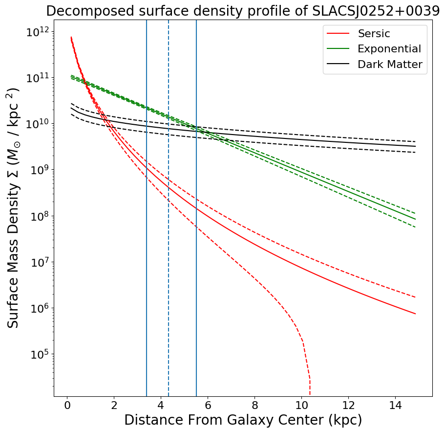 Figure 1
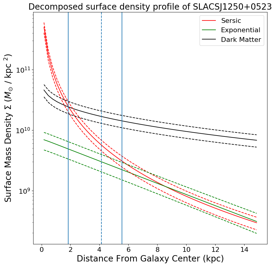 Figure 2
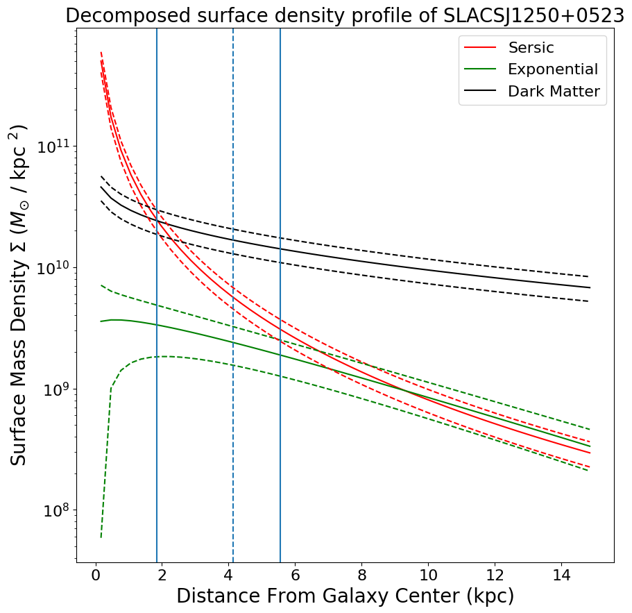 Figure 3
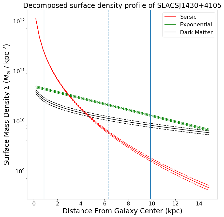 Figure 4
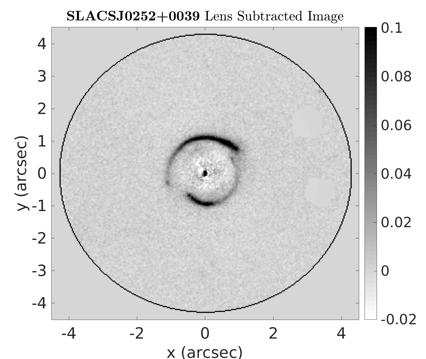 Figure 5
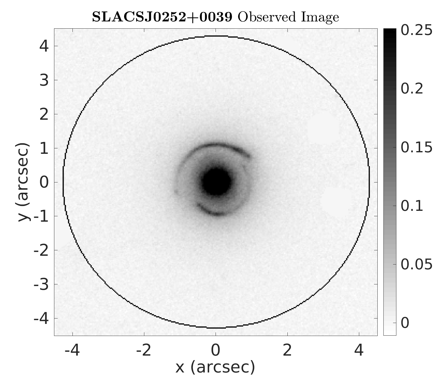 Figure 6
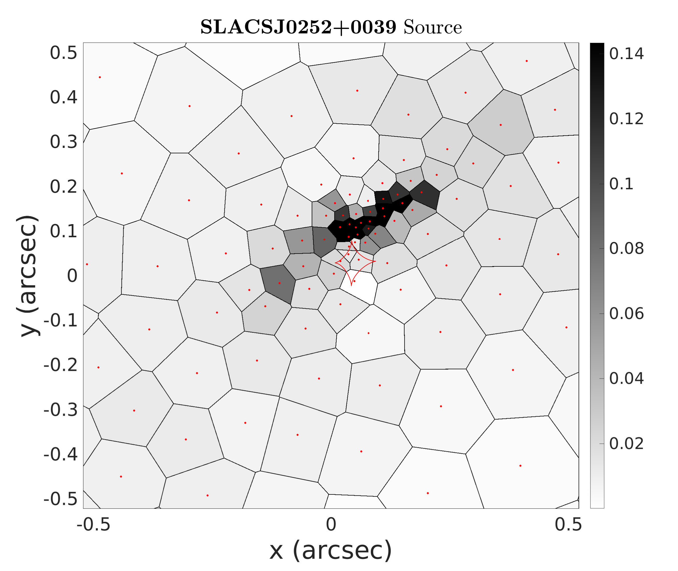 Figure 7
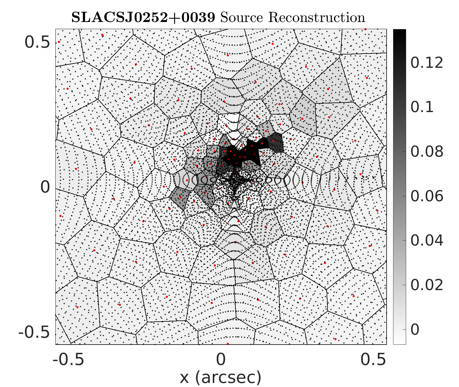 Figure 8
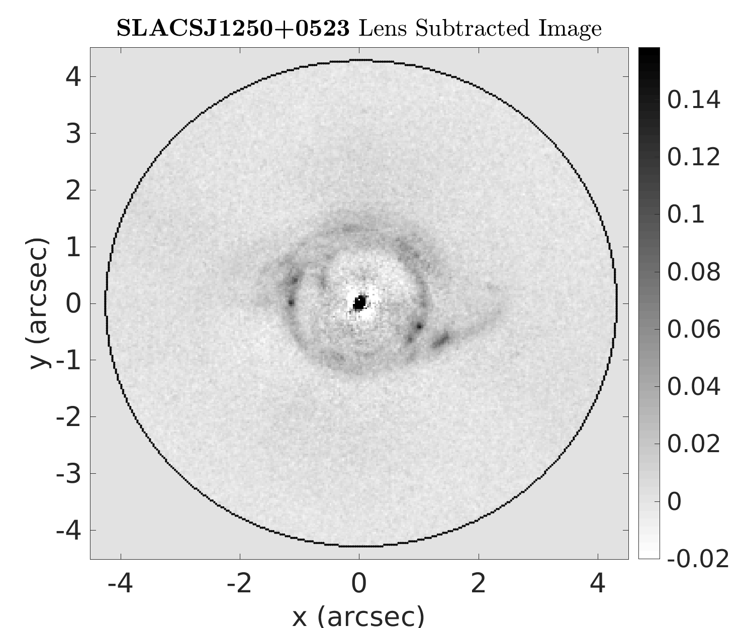 Figure 9
 Figure 10
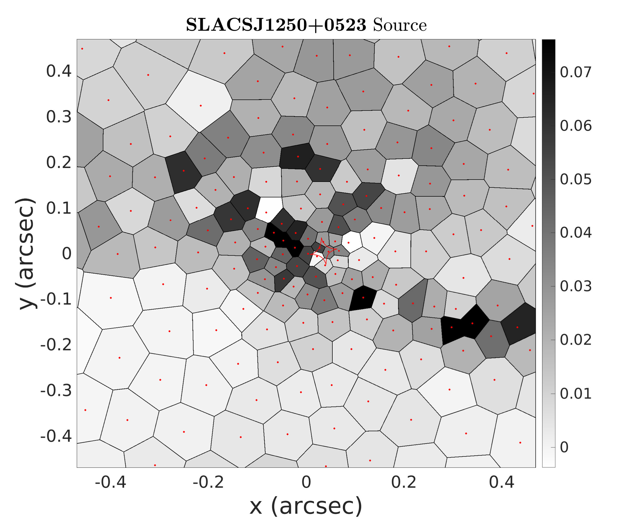 Figure 11
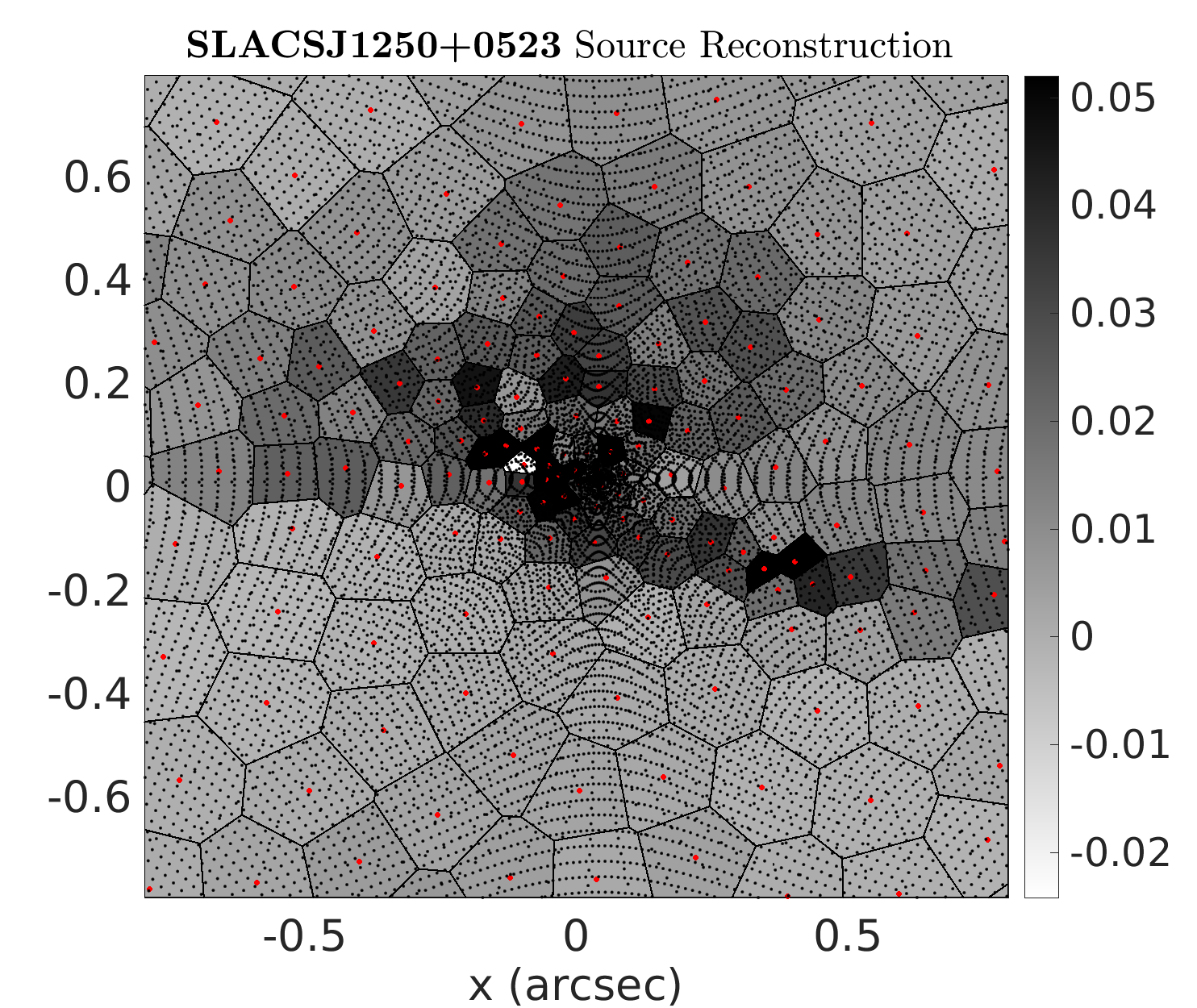 Figure 12
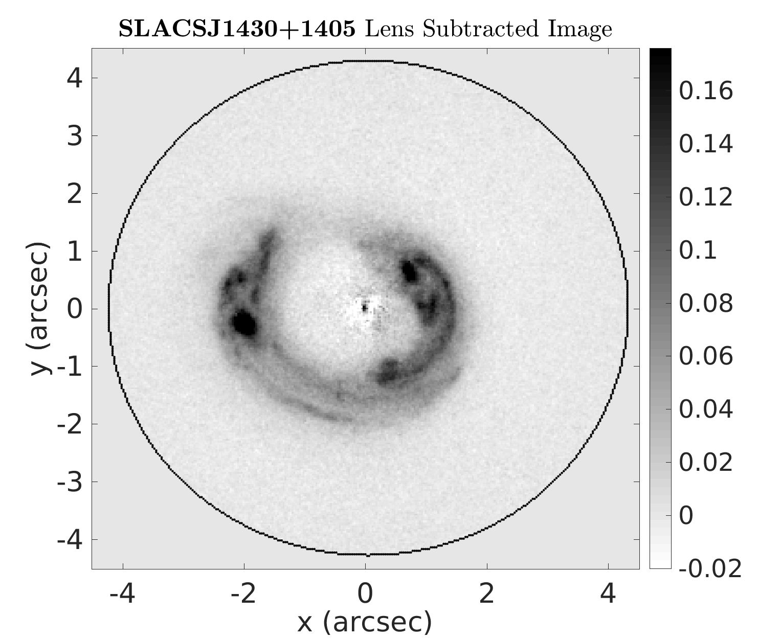 Figure 13
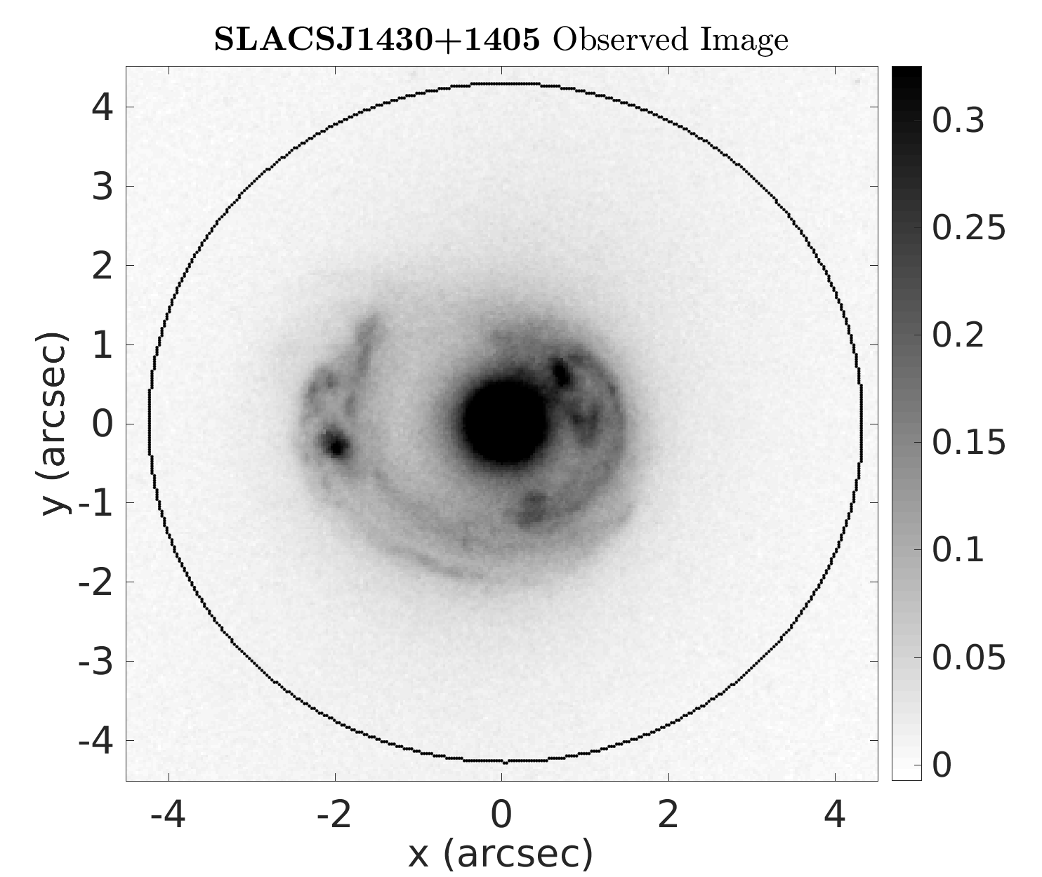 Figure 14
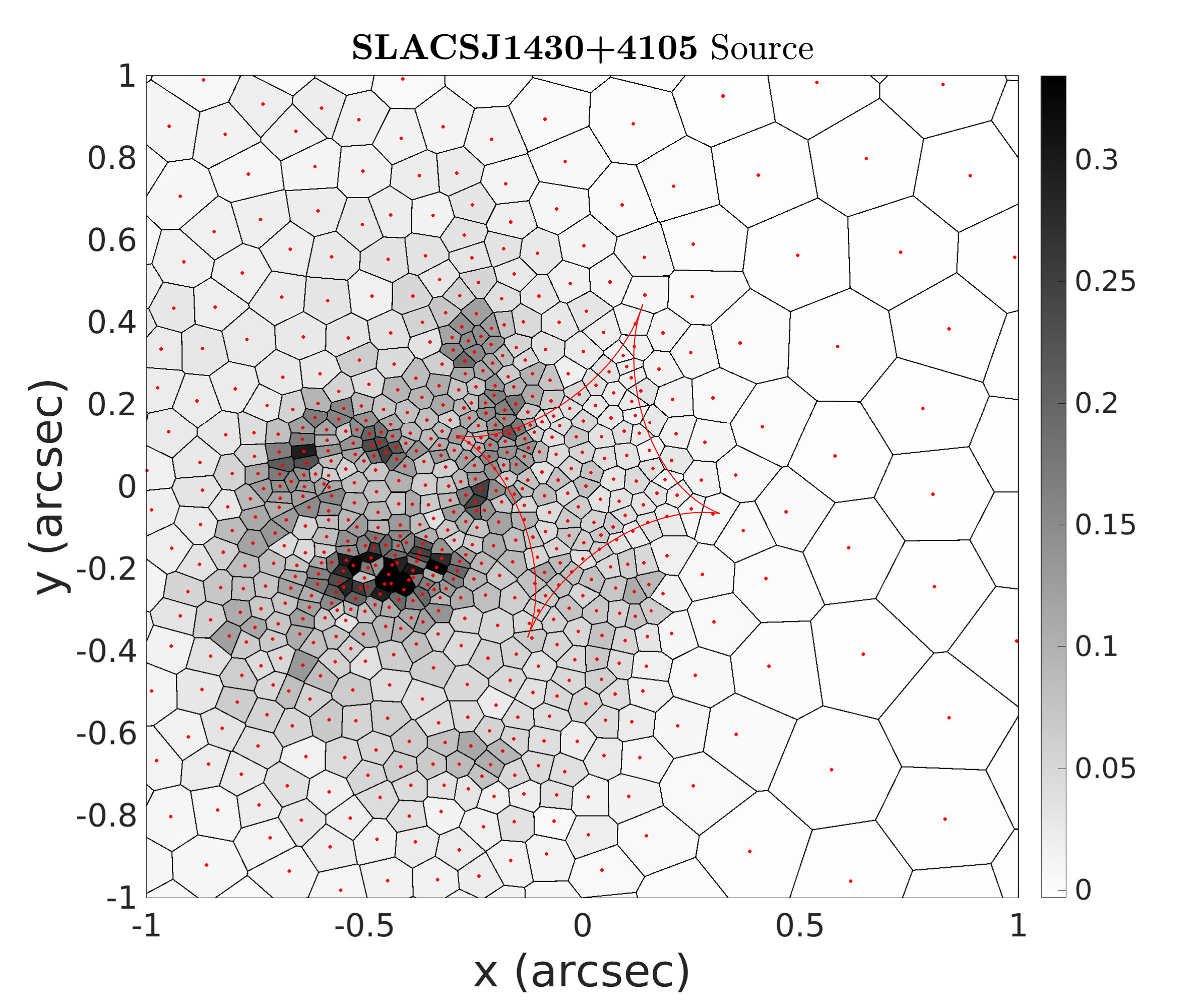 Figure 15
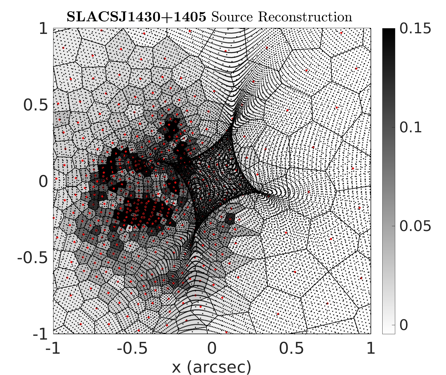 Figure 16
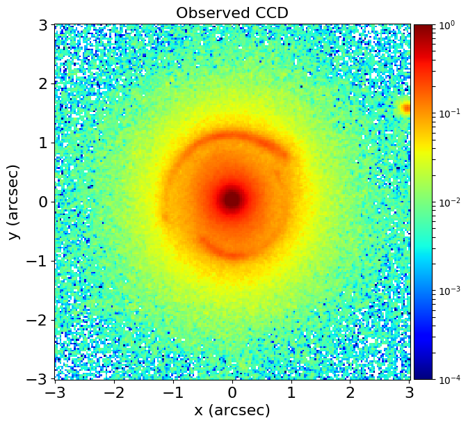 Figure 17
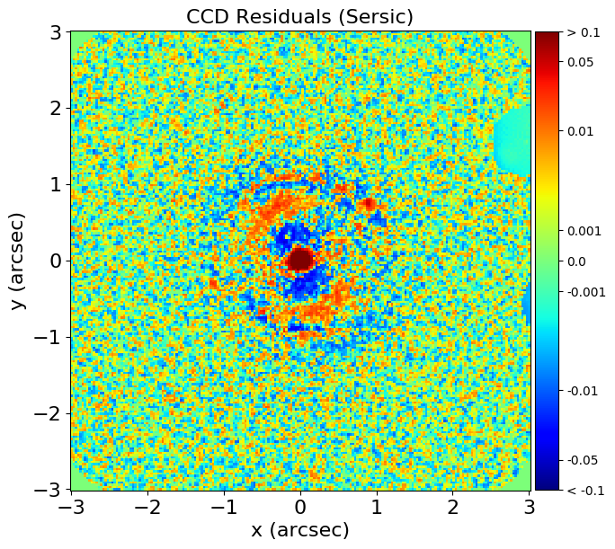 Figure 18
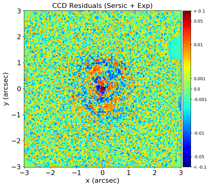 Figure 19
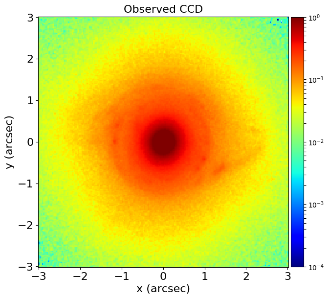 Figure 20
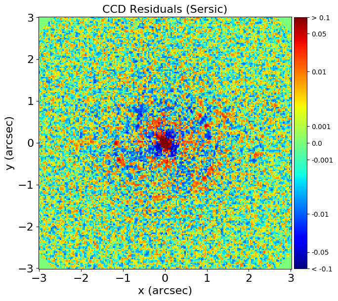 Figure 21
 Figure 22
 Figure 23
 Figure 24
 Figure 25
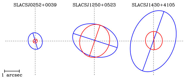 Figure 26
| Target name | RA | Dec | (km/s) | Near a cluster? | ||
|---|---|---|---|---|---|---|
| SDSSJ0252+0039 (SLACS1) | 02 5245.21 | +00∘3958 | 0.2803 | 0.9818 | - | |
| SDSSJ1250+0523 (SLACS2) | 12 5028.26 | +05∘2349 | 0.2318 | 0.7953 | - | |
| SDSSJ1430+4105 (SLACS3) | 14 3004.10 | +41∘0557 | 0.2850 | 0.5753 | MaxBCGJ217.49493+41.10435 () |
| Target name | (obs.) | (”) | (b/a) | (∘) | (SIE) | (SIE) | (Chab) | (Sal) | ||||||
|---|---|---|---|---|---|---|---|---|---|---|---|---|---|---|
| SDSSJ0252+0039 (SLACS1) | 18.04 | 1.39 | 0.94 | 97.2 | 11.25 | 1.04 | 0.93 | 106.2 | 3 | |||||
| SDSSJ1250+0523 (SLACS2) | 16.70 | 1.81 | 0.97 | 114.8 | 11.26 | 1.13 | 0.96 | 130.8 | 5 | |||||
| SDSSJ1430+4105 (SLACS3) | 16.87 | 2.55 | 0.79 | 120.7 | 11.73 | 1.52 | 0.68 | 111.7 | 6 |
| Model | Compo | ||||
| Represents | Parameters | ||||
| Sersic | Light + | Stellar Matter | (,) - profile center | - axis ratio | - orientation |
| Mass | - Intensity | - Effective Radius | - Sersic index | ||
| - Mass-to-Light Ratio | - Radial Gradient | ||||
| Exponential () | ” | ” | Identical to Sersic with fixed | ||
| Singular Isothermal | Mass | Total (Stellar | (,) - profile center | - axis ratio | - orientation |
| Ellipsoid (SIE) | + Dark Matter) | - Einstein Radius | |||
| Singular Isothermal Sphere (SIS) | ” | ” | Identical to SIE with fixed and omitted | ||
| Spherical NFW () | ” | Dark Matter | (,) - profile center | ||
| - Halo normalization | - Scale radius (fixed to 30 kpc) | ||||
| Elliptical NFW () | ” | ” | (,) - profile center | ||
| - Halo normalization | - Scale radius (fixed to 30 kpc) | ||||
| Generalized spherical NFW () | ” | ” | (,) - profile center | - inner slope | |
| - Halo normalization | - Scale radius (fixed to 30 kpc) | ||||
| Shear | ” | Line-of-sight | - magnitude | - orientation | |
| Target Name | Mass | ||||
|---|---|---|---|---|---|
| Mass-to-light Ratio | Second Light Component Profile | Single Sersic | Sersic + Halo | ||
| (shared geometry) | |||||
| Total | N/A | Exponential | 212290.8 | 212858.4 | |
| Decomposed | Shared | Exponential | 212273.4 | 212812.6 | |
| Total | N/A | Exponential | 216990.6 | 217214.5 | |
| Decomposed | Shared | Exponential | 217074.0 | 217180.3 | |
| Total | N/A | Exponential | 217423.3 | 217720.7 | |
| Decomposed | Shared | Exponential | 217110.8 | 217645.2 |
| Target Name | Mass | ||||
|---|---|---|---|---|---|
| Mass-to-light Ratio | Second Component Exponential | Second Component Sersic | Sersic Index | ||
| Total | N/A | 212858.4 | 212855.5 | ||
| Decomposed | Shared | 212812.6 | 212791.4 | ||
| Total | N/A | 217214.5 | 217189.2 | ||
| Decomposed | Shared | 217180.3 | 217172.2 | ||
| Total | N/A | 217720.7 | 217721.3 | ||
| Decomposed | Shared | 217645.2 | 217640.2 |
| Target Name | Mass | ||||||
|---|---|---|---|---|---|---|---|
| Mass-to-light Ratio | Second Light Component Profile | Sersic + Halo | |||||
| Sersic + Halo | (shared geometry) | ||||||
| Sersic + Halo | |||||||
| Sersic + Halo | |||||||
| (independent geometry) | |||||||
| Total | N/A | Exponential | 212858.4 | 212912.7 | 212870.2 | 212890.7 | |
| Decomposed | Shared | Exponential | 212812.6 | 212865.5 | 212804.1 | 212871.3 | |
| Decomposed | Independent | Exponential | 212819.4 | 212867.3 | 212861.7 | 212862.5 | |
| Total | N/A | Exponential | 217214.5 | 217228.1 | 217223.5 | 217249.0 | |
| Decomposed | Shared | Exponential | 217180.3 | 217194.0 | 217210.9 | 217219.7 | |
| Decomposed | Independent | Exponential | 217183.2 | 217216.6 | 217205.2 | 217240.4 | |
| Total | N/A | Exponential | 217720.7 | 217840.3 | 217753.2 | 217852.4 | |
| Decomposed | Shared | Exponential | 217645.2 | 217780.8 | 217663.0 | 217804.7 | |
| Decomposed | Independent | Exponential | 217676.5 | 217823.4 | 217694.5 | 217876.0 |
| Target Name | Mass | ||||||
|---|---|---|---|---|---|---|---|
| Independent ? | Rotationally Offset? | Centrally Offset? | No Radial Variation | Radial Variation | |||
| Radial Variation | () | ||||||
| () | |||||||
| Decomposed | Yes | Yes | No | 212867.3 | 212867.4 | 212847.4 | |
| Decomposed | Yes | Yes | Yes | 217246.6 | 217276.0 | 217300.9 | |
| Decomposed | Yes | Yes | Yes | 217922.6 | 217918.8 | 217931.1 |
| Target Name | Mass | ||||
|---|---|---|---|---|---|
| (free ) | (free & ) | ||||
| Decomposed | 212854.8 | 212860.1 | 212853.7 | 212852.8 | |
| Decomposed | 217246.7 | 217259.5 | 217264.2 | 217255.9 | |
| Decomposed | 217922.0 | 217925.5 | 217928.6 | 217930.1 |
| Target Name | Radius (kpc) | Total Mass () | Stellar Mass () | Mass () | Mass () | Dark Matter Mass () |
|---|---|---|---|---|---|---|
| 10.0 | ||||||
| 500.0 | ||||||
| 10.0 | ||||||
| 500.0 | ||||||
| 10.0 | ||||||
| 500.0 |
| Target Name | Mass | |||||
|---|---|---|---|---|---|---|
| Mass-to-light Ratio | Parameters | |||||
| Total | N/A | |||||
| Decomposed | N/A | |||||
| Total | N/A | |||||
| Decomposed | N/A | |||||
| Total | N/A | |||||
| Decomposed | N/A |
| Target Name | Mass | |||||
|---|---|---|---|---|---|---|
| Mass-to-light Ratio | Parameters | |||||
| Total | N/A | |||||
| Decomposed | Single | |||||
| Total | N/A | |||||
| Decomposed | Single | |||||
| Total | N/A | |||||
| Decomposed | Single | |||||
| Target Name | Mass | |||||
|---|---|---|---|---|---|---|
| Mass-to-light Ratio | Parameters | |||||
| Total | N/A | |||||
| Decomposed | Single | |||||
| Decomposed | Independent | |||||
| Total | N/A | |||||
| Decomposed | Single | |||||
| Decomposed | Independent | |||||
| Total | N/A | |||||
| Decomposed | Single | |||||
| Decomposed | Independent | |||||
| Target Name | Mass | |||||
| Mass-to-light Ratio | Parameters | |||||
| Decomposed | Single | |||||
| Decomposed | Independent | |||||
| Decomposed | Single | |||||
| Decomposed | Independent | |||||
| Decomposed | Radial Gradient | |||||
| Decomposed | Single | |||||
| Decomposed | Independent |
| Target Name | Dark Matter | ||||
|---|---|---|---|---|---|
| Parameters | |||||
Peer Reviews
No public reviews on file for this paper yet. If you reviewed it on a platform where reviews are public (OpenReview, ICLR, NeurIPS, ICML), you can paste yours below so the community can read it here.
Videos
No videos yet. Explain this paper in a talk, walkthrough, or lecture? Add one.
Galaxy structure with strong gravitational lensing:
decomposing the internal mass distribution of massive elliptical galaxies
James. W. Nightingale1, Richard J. Massey1, David R. Harvey2, Andrew P. Cooper1,3, Amy Etherington1, Sut-Ieng Tam1 & Richard G. Hayes1
1Centre for Extragalactic Astronomy, Department of Physics, Durham University, South Road, Durham, DH1 3LE, UK
2Laboratoire d’Astrophysique, EPFL, Observatoire de Sauverny, 1290 Versoix, Switzerland
3Institute of Astronomy and Department of Physics, National Tsing Hua University, Hsinchu 30013, Taiwan e-mail: [email protected]
(March 2, 2024)
Abstract
We investigate how strong gravitational lensing can test contemporary models of massive elliptical (ME) galaxy formation, by combining a traditional decomposition of their visible stellar distribution with a lensing analysis of their mass distribution. As a proof of concept, we study a sample of three ME lenses, observing that all are composed of two distinct baryonic structures, a ‘red’ central bulge surrounded by an extended envelope of stellar material. Whilst these two components look photometrically similar, their distinct lensing effects permit a clean decomposition of their mass structure. This allows us to infer two key pieces of information about each lens galaxy: (i) the stellar mass distribution (without invoking stellar populations models) and (ii) the inner dark matter halo mass. We argue that these two measurements are crucial to testing models of ME formation, as the stellar mass profile provides a diagnostic of baryonic accretion and feedback whilst the dark matter mass places each galaxy in the context of LCDM large scale structure formation. We also detect large rotational offsets between the two stellar components and a lopsidedness in their outer mass distributions, which hold further information on the evolution of each ME. Finally, we discuss how this approach can be extended to galaxies of all Hubble types and what implication our results have for studies of strong gravitational lensing.
keywords:
galaxies: structure — gravitational lensing
††pagerange: Galaxy structure with strong gravitational lensing: decomposing the internal mass distribution of massive elliptical galaxies–B††pubyear: 2018
1 INTRODUCTION
The work of Hubble (1926) famously classified galaxies into three groups: ellipticals, spirals and irregulars. Today, using samples of hundreds of thousands of galaxies, these classifications have been broadly established to hold across all galaxies, in the local Universe (Hoyos et al. 2011; Vika et al. 2013; Vulcani et al. 2014) and at high redshift (Buitrago et al. 2008; Chevance et al. 2012; Bruce et al. 2012; Van Der Wel et al. 2012). The bulk structure of a galaxy can be quantified by its one-dimensional projected surface brightness profile. The Sersic function, , (de Vaucouleurs 2005; Sersic 1968) has proven extremely useful for this purpose across the entire Hubble sequence. The bulk of the light in a typical elliptical galaxy is well described by and an exponential disk structure by . Although most galaxies can be labelled with a specific morphology on the Hubble diagram without much ambiguity, they can also exhibit sub-dominant structures with other morphologies (see Graham 2013). For example, spirals have bulges (Thomas & Davies 2006; MacArthur, González & Courteau 2009), ellipticals have disks (Thomas A. Oosterloo, Raffaella Morganti, Elaine M. Sadler, Daniela Vergani & Caldwell 2002; Bluck et al. 2014) and irregulars may show signs of both bulges and disks (Margalef-Bentabol et al. 2016). This has motivated descriptions that use multiple Sersic profiles (Lackner & Gunn 2012; Bruce et al. 2014; Vika et al. 2014; Kennedy et al. 2016) to decompose galaxies into their constituent physical structures.
Fitting the light distribution of a galaxy with a superposition of light profiles is a challenging and highly degenerate problem (e.g. Häußler et al. 2013). For example, the extended wings of a central bulge can be difficult to separate from structures further out (e.g. a disk), as they blend with one another and the background sky emission. Bulges, disks and bars may all appear as compact central structures in a galaxy, which are hard to decouple from one another (Kormendy 1995). Absorption of light by dust can also impact the fit, leading to more ambiguities in the interpretation of a galaxy’s structure (Rest et al. 2001; Lauer et al. 2005).
Using integral field spectroscopy (IFS), the SAURON (Bacon et al. 2001) and ATLAS3D (Cappellari et al. 2011) surveys demonstrated the importance, when trying to infer a galaxy’s structure, of having data sensitive to its mass. For example, Emsellem et al. (2004; 2007; 2011) found that of galaxies in a volume-limited sample showed some level of ordered rotation in their kinematics despite showing no signs of a disk in their light (Krajnović et al. 2011; 2013). IFS data also reveal that biases in the inferred galaxy structure may arise due to the 3D inclination (Devour & Bell 2017) and the triaxiality (Méndez-Abreu et al. 2010a; b) of the different structures within galaxies, which limits inferences based on their 2D projected morphologies (Cappellari 2008; Emsellem et al. 2011; Weijmans et al. 2014).
In this work, we propose that strong gravitational lensing can both mitigate the degeneracies that arise when fitting a galaxy’s 2D light distribution and provide key insight on its underlying physical mass structure. Strong lensing is the deflection of light from a background source around a foreground lens galaxy, giving rise to multiple images of the source with characteristic distortions (see Kochanek (2004) for an overview). These distortions encode information on the foreground lens’s mass distribution and make it easier to separate the different galaxy components in comparison to using photometry alone. Conveniently, lensing data can be extracted from the same CCD imaging as the photometry, in contrast to IFS data which must be obtained separately: at significant cost in observing time, and typically at much coarser spatial resolution.
For this proof-of-concept study, we use our open-source lens modeling software PyAutoLens111https://github.com/Jammy2211/PyAutoLens (Nightingale & Dye 2015; Nightingale, Dye & Massey 2018) to fit the projected optical luminosity distribution of three isolated massive elliptical (ME) galaxies with velocity dispersions of -, whilst simultaneously constraining their underlying mass structure via a strong lensing analysis. We recover the distribution of both light and mass in projection along the line of sight, enabling these two inferences of galaxy structure to be compared directly and circumventing ambiguities due to dust. Crucially, this approach allows us to confirm whether or not features apparent in the light distribution correspond to genuine physical structures.
This question is central to tests of ME galaxy formation in the LCDM cosmology, which predicts that they assemble their stellar mass both by dissipative star formation and by mergers with other galaxies. Each of these processes should give rise to physically distinct components in the phase-space structure of MEs that may have observable signatures in their stellar mass surface density profiles. In particular, active galactic nuclei (AGN) activity at the centre of haloes more massive than is thought to act as a ‘thermostat’ that shuts down in-situ growth of their central galaxy by suppressing radiative cooling of fresh cold gas from a hot circumgalactic reservoir (Croton et al. 2006; Bower et al. 2006; 2017). The progenitors of present-day MEs form rapidly in overdense regions at z\lower 2.15277pt\hbox{;\buildrel>\over{\sim};}2–, hence the stars they form in situ (i.e. before AGN suppression) are characterised by high metallicity and high phase space density (Baugh, Cole & Frenk 1996; Hopkins et al. 2005; De Lucia et al. 2006). By the present day these stellar populations have old ages and red colours.
Although in situ star formation is suppressed in MEs, DM mass growth continues in an approximately self-similar fashion (e.g. Guo & White 2008). The most massive halos at the present day, which are much more massive than the ‘threshold’ mass for AGN suppression, coalesce relatively recently. Their immediate progenitor halos are themselves likely to be above the threshold mass, and hence also to host gas-poor galaxies with ‘red and dead’ metal-rich stellar populations. This leads to a picture in which the bulk of stellar mass in MEs is assembled through dissipationless mergers of several equally important fragments. These fragments have a broad range of DM halo masses but a narrow range of stellar masses (De Lucia & Blaizot 2007).
The structure of the resulting MEs (represented to lowest order by the scale and shape of their surface brightness profile) is therefore dominated by the ‘initial conditions’ and gravitational dynamics of these mergers, in which DM plays a dominant role (e.g. Cole et al. 2000; Boylan-Kolchin, Ma & Quataert 2006; Naab, Johansson & Ostriker 2010; Hilz, Naab & Ostriker 2013; Laporte et al. 2013). Broadly speaking, forward models of ME formation predict a composite structure arising from the superposition of phase-mixed stellar debris from each progenitor, each with a characteristic profile and scale (similar to the assembly of stellar halos around less massive galaxies described by Amorisco 2015). For typical ME assembly histories, the dominant accreted components are expected to have similar amplitude, shape and radial extent (e.g. Cooper et al. 2013; 2015). Consequently, the aggregate stellar density profile is (on average) unlikely to show strong inflections that correspond to transitions between regions of the galaxy dominated by debris from different progenitors. Indeed, observations (e.g. Kormendy et al. (2009)) show that to good approximation, the overall structure may be described as a single component with Sersic n\lower 2.15277pt\hbox{;\buildrel>\over{\sim};}4 (Schombert 2015).
The strongest observational features are therefore most likely to arise between the more extended aggregate accreted component and the centrally concentrated component, corresponding to an in-situ, high redshift ‘nugget’ (with much higher phase space density as the result of dissipative formation). Sufficiently deep imaging of local MEs observe this (Huang et al. 2013; 2018b; Spavone et al. 2017), including components with different ellipticities, orientations (isophotal twists) (Oh, Greene & Lackner 2016a; b) and centers (Goullaud et al. 2018). Spectroscopic studies of MEs are also consistent with this picture, whereby the stellar ages and alpha-element abundances of their central regions are both observed to increase with velocity dispersion (Raskutti, Greene & Murphy 2014; Greene et al. 2013; 2015), trends which appear washed out at larger radii where stars are anticipated to have been more recently accreted222These expectations for accretion on to MEs are significantly different to those for Milky Way-like galaxies, which correspond to the regime of in situ dominated growth in lower-mass halos largely unaffected by AGN feedback. In that regime, the analogous accreted stellar component (the stellar halo) is expected to be dominated by only one or two accretion events of high mass ratio, and to comprise only a small fraction of the total mass. Stellar halo progenitors arrive on more circular orbits (giving rise to streams and other unrelaxed structures) and consist of stellar populations very different to those of the central galaxy (Bullock & Johnston 2005; De Las Aguas Robustillo Cortés, González & Verdugo 2017; Amorisco 2015)..
Observations such as these have been interpreted as evidence for a model in which an ‘outer envelope’ arises from prolonged and significant accretion onto a high-density stellar core. This model, often referred to as ‘two phase’ assembly (e.g. Oser et al. 2010), is broadly equivalent to the predictions of the LCDM models described above in the ME regime. Examples of massive compact ellipticals, thought to correspond to these dissipative cores before significant accretion, have been observed at high redshift but are extremely rare at the present day (e.g. Trujillo et al. 2006; Szomoru et al. 2011; Oldham et al. 2017). Overall, observations appear to be consistent with the evolution of the galaxy population as a whole predicted by LCDM models, once selection effects are taken into account (Laporte et al. 2013; Xie et al. 2015; Furlong et al. 2017; Roy et al. 2018). Furthermore, indirect tracers of dark matter mass (e.g. environment or size) detect correlations consistent with the above picture in populations of elliptical galaxies (Lani et al. 2013; Sonnenfeld et al. 2015; Huang et al. 2018a).
Nevertheless, decomposing MEs into multiple components remains very challenging, because their two (or more) superposed elliptical components (with similar stellar populations) are often well described by a single elliptical profile. This makes them the ideal case-study for investigating how strong lensing can aid the decomposition of a galaxy’s structure. We will demonstrate that strong lens modeling: (i) allows us to confirm that the structures we see visualally correspond to genuine mass components; (ii) provides direct access to the stellar mass distribution of each component (without stellar population modeling) and; (iii) infers the central ( kpc) dark matter halo mass of each galaxy. With a sample of just objects, our conclusions primarily focus on discussing the utility of this method. In the future, existing samples of hundreds of lenses will enable a direct test of LCDM expectations for the assembly of MEs, in particular the fundamental relationship between halo mass, stellar mass distribution and galaxy history. Future samples of 100000 strong lenses (Collett 2015) will allow such an analysis to be generalised over the entire Hubble sequence.
This paper is structured as follows. In §2, we describe our sample of three ME galaxies selected for detailed study. In §3, we describe the PyAutoLens method for simultaneous photometric and strong lensing analysis. In §4, we investigate the mass structure of our lenses. In §5, we discuss the implications of our measurements, and we give a summary in §6. We assume a Planck 2015 cosmology throughout (Planck Collaboration et al. 2015).
2 Data Reduction and Lens Sample
2.1 HST data reduction
We adopt a modified data reduction pipeline that uses a combination of in-house tools and those from the standard Space Telescope Science Institute library. We first correct images for charge transfer inefficiency using the arCTIc software (Massey et al. 2010; 2014). We then bias subtract, flat field and co-add multiple exposures using the calacs and astrodrizzle packages to create a final data product. Following Rhodes et al. (2007), we combine the images using a square drizzle kernel and a pixel fraction of 0.8, to a final pixel scale of . To determine the Point Spread Function (PSF) of this final image, we measure the focus of the telescope during each exposure, via the quadrupole moments of stars throughout that exposure (c.f. Harvey et al. 2015), then coadd (appropriately rotated) TinyTim models of each exposure’s PSF (Krist, Hook & Stoehr 2011). We store a single, 2D model of the combined PSF at the location of the lens, with a matching pixel scale of 0.03, with the peak of the PSF the centre of a pixel.
This procedure produces a sky-subtracted, stacked image of each lens, which is used for the analysis. The variance in each pixel is estimated as , where is the estimated variance in the background and is the total counts detected in pixel (accounting for the variation in exposure time due to dithering). The variances and background sky level are included as part of the modeling procedure (see N18).
2.2 Lens Sample
The preliminary sample of three lenses used in this work is taken from the Sloan Lens ACS Survey (SLACS, e.g. Bolton et al. 2008), where galaxies were initially selected from the Sloan Digital Sky Survey (SDSS) main (Richards et al. 2002) and luminous red galaxy (LRG, Eisenstein et al. 2001) catalogues, as containing spectral emission lines from more than one redshift in a single fibre. The SLACS lens galaxies therefore primarily consist of ME galaxies with no known differences to other similar galaxies in the main or LRG parent samples (e.g. Bolton et al. 2006; Treu et al. 2009), other than a bias towards higher total mass.
Imaging of SLACS lenses is available across a range of wavelengths and spatial resolutions. We analyse monochromatic images, and have two primary considerations in selecting a waveband: (i) high spatial resolution to better constrain the lens model and; (ii) longer wavelength coverage to be more sensitive to the lens galaxy’s old stellar populations (which contribute most significantly to its mass). We choose HST/Advanced Camera for Surveys (ACS) imaging taken with the F814W filter, which provides high-resolution imaging at rest-frame near-infrared (NIR) wavelengths. We also require that this imaging is available with an exposure time of at least one Hubble orbit. This work is focused on showing what can be measured for individual systems, so selection effects are not important for this work’s conclusions.
These criteria yield a sample of 40 ME lenses, which SDSS spectroscopy separates into three bins of velocity dispersion (uncorrected for aperture effects): low (230$$<$$\sigma_{\mathrm{SDSS}}$$<$$270 km/s), intermediate (310$$<$$\sigma_{\mathrm{SDSS}}$$<$$350 km/s) and high (\sigma_{\mathrm{SDSS}}$$>$$360 km/s). We select one lens randomly from each bin, resulting in the lenses SDSSJ0252+0039 (low , hereafter SLACS1), SDSSJ1250+0523 (intermediate , hereafter SLACS2) and SDSS1430+4105 (high , hereafter SLACS3). None are cD or Brightest Cluster Galaxies, but SLACS3 is in the field of a nearby cluster (Treu et al. 2009). SLACS1 and SLACS3 were both observed in HST programme GO-10886 and SLACS2 in programme GO-10494. Table 1 gives a summary of each lens’s observed properties (Bolton et al. 2008), including , the source and lens redshifts, and . Table 2 shows the results of previous SLACS analyses – in particular photometry, stellar population modeling and stellar dynamics (Auger et al. 2010a; b), and mass modeling (Bolton et al. 2008).
2.3 Sample Description
Based on previous SLACS results (tables 1 and 2) and the reduced images in figure 1 we give a brief description of each lens in our sample. For clarity, figure 1 also shows an image of the background galaxies after subtracting the lens light (middle column), and de-lensed reconstructions of that source (right column), which are computed using the highest likelihood lens model found by PyAutoLens (which is described next). Neither the lens subtraction nor source reconstruction show large differences when plotted using other high-likelihood lens models, thus these images are indicative of the analysis for any good lens model.
2.3.1 SLACS1
SLACS1 is pictured in the top row of figure 1. The lens galaxy has an elliptical visual morphology extending smoothly from its centre to ”. The lensed source shows arcs above and below the lens galaxy, which the source reconstruction reveals are a compact knot of light just outside the fold caustic. This lens is therefore a doubly imaged system with minimal extended structure in the source’s surface brightness.
The lens is the lowest mass galaxy in our sample, with an Einstein Mass within its Einstein Radius kpc, a stellar mass (Chabrier IMF) and a velocity dispersion km/s. This translates to a stellar mass fraction within of for a Charbrier IMF. Notably, it has the lowest density slope (inferred via lensing and stellar dynamics) in the whole SLACS sample, with a value .
The HST imaging of SLACS1 had three faint galaxies not associated with the lens or source which overlapped the masked region within which the analysis is performed. These were subtracted using a linear light profile fitting routine and their pixel variances were increased to infinity such that the analysis ignored them. The object at was included in the lens model as a singular isothermal sphere fixed to these coordinates. However, omitting it was found to have no impact on the results discussed in this work.
2.3.2 SLACS2
SLACS2 is pictured in the middle row of figure 1. The lens galaxy again visually shows one smooth extended component, but extending further, to ”. The lensed source is complex, with a near-circular ring of light, two radial arcs protruding into the lens’s centre and six distinct flux peaks. The source reconstruction reveals two galaxies either side of the inner caustic, with features indicative of merging visible in their extended surface brightness profiles, in particular a disrupted tidal tail trailing each source. These tails form the inner ring of light, radial arcs and extended arcs outside the lens in the image-plane.
Although this lens was chosen from the intermediate bin with a value km/s, it turns out to be the highest mass object in our sample with within kpc and . Its stellar mass fraction is also the highest in our sample with . Finally, its density slope makes it one of the steeper slopes in SLACS and the steepest in our sample.
2.3.3 SLACS3
SLACS3 is pictured in the bottom row column of figure 1. The lens again shows one smooth extended component. The source shows two bright knots of light in a double image configuration, which the source reconstruction shows is the source galaxy’s central bulge. However, also visible is a wealth of additional extended structure surrounding this bulge, which in the image-plane forms multiple giant arcs around the lens. The source may be a face-on spiral galaxy, where the arms on the opposite side of the caustic are not visible due to the reduced magnification. Alternatively, it is a complex merging system.
This object has within kpc, and km/s. It has a stellar mass fraction and density slope . Unlike the other lenses in our sample, SLACS3 is near a cluster (Treu et al. 2009).
3 Method
When an extended source is gravitationally lensed, light rays emanating from different regions of the source galaxy trace different paths through the lens galaxy. This provides a projected and extended view of the lens’s gravitational potential, information which can be recovered with knowledge of the source’s unlensed light distribution. Thus, we are exploiting the lensed source’s surface brightness profile, in contrast to the previous photometric studies of SLACS lenses which used only the source’s position to measure the lens galaxy’s Einstein Mass, (e.g. Auger et al. 2010b). It is this exploitation of the source’s extended information which allows us to constrain the lens’s underlying mass structure.
To perform this analysis we use our new lens modeling software PyAutoLens333The PyAutoLens software is open-source and available from https://github.com/Jammy2211/PyAutoLens. The results in this work were computed using an earlier Fortran build of AutoLens, which is described in Nightingale, Dye & Massey (2018, N18 hereafter), building on the works of Warren & Dye (2003, WD03 hereafter), Suyu et al. (2006, S06 hereafter) and Nightingale & Dye (2015, N15 hereafter). We refer readers to these works for a full description of PyAutoLens. Key points to note are:
the lens galaxy’s light and mass distributions are fitted simultaneously; 2. 2.
the source’s surface brightness distribution is reconstructed on an adaptive pixel-grid (see the right column of figure 1); 3. 3.
the Bayesian framework of S06 is used to objectively determine the most probable source reconstruction, and the complexity of the lens model is also chosen objectively via Bayesian model comparison (using MultiNest; Feroz, Hobson & Bridges 2009; Park et al. 2018); 4. 4.
the method is fully automated and requires no user intervention (after a brief initial setup) for the analysis presented in this work.
The reference list from the paper itself. Each links out to its DOI / PubMed record.
- 1Amorisco (2015) Amorisco N. C., 2015, Monthly Notices of the Royal Astronomical Society, 464, 2882
- 2Auger et al . (2010 a) Auger M. W., Treu T., Bolton A. S., Gavazzi R., Koopmans L. V., Marshall P. J., Moustakas L. A., Burles S., 2010 a, Astrophysical Journal, 724, 511
- 3Auger et al . (2010 b) Auger M. W., Treu T., Bolton A. S., Gavazzi R., Koopmans L. V., Marshall P. J., Moustakas L. A., Burles S., 2010 b, Astrophysical Journal, 724, 511
- 4Bacon et al . (2001) Bacon R. et al., 2001, Monthly Notices of the Royal Astronomical Society, 326, 23
- 5Baugh, Cole & Frenk (1996) Baugh C. M., Cole S., Frenk C. S., 1996, Monthly Notices of the Royal Astronomical Society, 283, 1361
- 6Birrer et al . (2019) Birrer S. et al., 2019, Monthly Notices of the Royal Astronomical Society, 484, 4726
- 7Bluck et al . (2014) Bluck A. F. L., Ellison S. L., Patton D. R., Simard L., Mendel J. T., Teimoorinia H., Moreno J., Starkenburg E., 2014, Ar Xiv e-prints, 000, 6
- 8Bolton et al . (2008) Bolton A. S., Burles S., Koopmans L. V. E., Treu T., Gavazzi R., Moustakas L. A., Wayth R., Schlegel D. J., 2008, The Astrophysical Journal, 682, 964