Lemniscates as Trajectories of Quadratic Differentials (I)
Faouzi Thabet

TL;DR
This paper explores polynomial and rational lemniscates as trajectories of quadratic differentials, providing new proofs for many classical results in complex analysis and geometric function theory.
Contribution
It introduces a novel approach by linking lemniscates to quadratic differentials, simplifying proofs of existing theorems.
Findings
Lemniscates can be characterized as trajectories of specific quadratic differentials.
Many classical lemniscate results are derived more straightforwardly.
The approach unifies geometric and analytical perspectives on lemniscates.
Abstract
In this note, we study polynomial and rational lemniscates as trajectories of related quadratic differentials. Many classic results can be then proved easily...
Click any figure to enlarge with its caption.
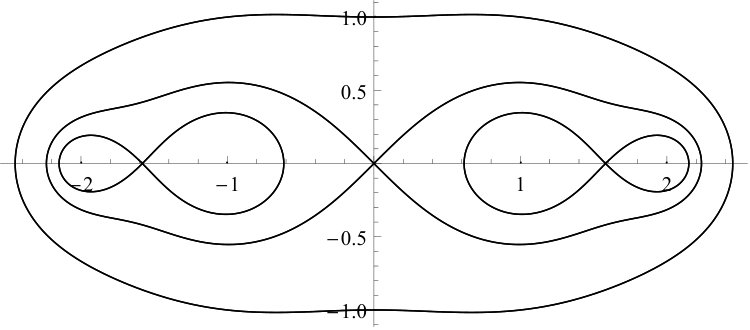 Figure 1
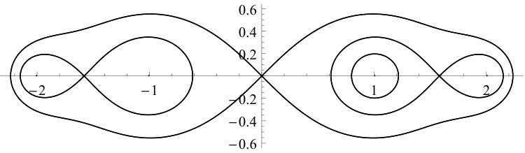 Figure 2
 Figure 3
 Figure 4
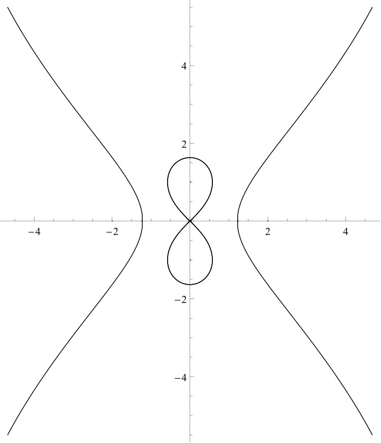 Figure 5
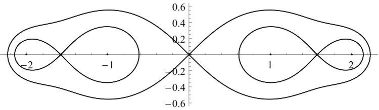 Figure 6
 Figure 7
 Figure 8
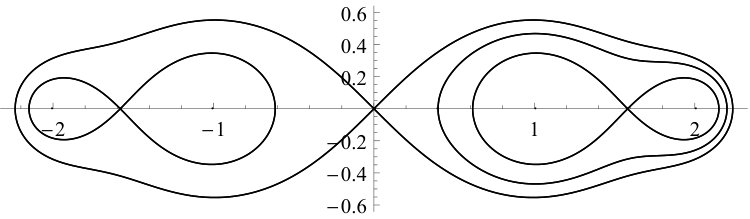 Figure 9
 Figure 10
 Figure 11
 Figure 12
Peer Reviews
No public reviews on file for this paper yet. If you reviewed it on a platform where reviews are public (OpenReview, ICLR, NeurIPS, ICML), you can paste yours below so the community can read it here.
Videos
No videos yet. Explain this paper in a talk, walkthrough, or lecture? Add one.
Taxonomy
TopicsNumerical methods for differential equations · Advanced Differential Equations and Dynamical Systems
Lemniscates as Trajectories of Quadratic Differentials
Faouzi Thabet
University of Gabes, Tunisia
Abstract
In this note, we study polynomial and rational lemniscates as trajectories of related quadratic differentials. Some classic results can be then proved easily…
2010 Mathematics subject classification: 30C10, 30C15, 34E05.
Keywords and phrases: Quadratic differentials. Lemniscates.Fingerprints.
1
A quadratic differential
Given a rational function where and are two co-prime complex polynomials, we consider the quadratic differential on the Riemann sphere :
[TABLE]
Finite critical points and *infinite critical points *of are respectively its zero’s and poles; all other points of are called regular points of
It is obvious that the partial fraction decomposition of is as follows :
[TABLE]
where is the multiplicity of the zero of We deduce that
[TABLE]
In other words, the zero’s of and are poles of order of with negative residue.
If
[TABLE]
(in particular, if ), then, with the parametrization , we get
[TABLE]
thus, is another double pole* *of with negative residue. If
[TABLE]
then is zero of with multiplicity greater than In the case
[TABLE]
is a regular point.
Horizontal trajectories (or just trajectories) of the quadratic differential are the zero loci of the equation
[TABLE]
or equivalently
[TABLE]
If is a horizontal trajectory, then the function
[TABLE]
is monotone.
The vertical (or, orthogonal) trajectories are obtained by replacing by in equation (3). The horizontal and vertical trajectories of the quadratic differential produce two pairwise orthogonal foliations of the Riemann sphere .
A trajectory passing through a critical point of is called critical trajectory. In particular, if it starts and ends at a finite critical point, it is called finite critical trajectory, otherwise, we call it an infinite critical trajectory.
If two different trajectories are not disjoint, then their intersection must be a zero of the quadratic differential.
The closure of the set of finite and infinite critical trajectories is called the critical graph of we denote it by
The local and global structures of the trajectories is well known (more details about the theory of quadratic differentials can be found in [5],[3], or [6]), in particular :
- •
At any regular point, horizontal (resp. vertical) trajectories look locally as simple analytic arcs passing through this point, and through every regular point of passes a uniquely determined horizontal (resp. vertical) trajectory of these horizontal and vertical trajectories are locally orthogonal at this point.
- •
From each zero with multiplicity of there emanate critical trajectories spacing under equal angle .
- •
Any double pole has a neighborhood such that, all trajectories inside it take a loop-shape encircling the pole or a radial form diverging to the pole, respectively if the residue is negative or positive.
- •
A trajectory in the large can be, either a closed curve not passing through any critical point (closed trajectory), or an arc connecting two critical points, or an arc that has no limit along at least one of its directions (recurrent trajectory).
The set consists of a finite number of domains called the domain configurations of For a general quadratic differential on a , there are five kind of domain configuration, see [3, Theorem3.5]. Since all the infinite critical points of are poles of order with negative residues, then there are three possible domain configurations:
- •
the Circle domain : It is swept by closed trajectories and contains exactly one double pole. Its boundary is a closed critical trajectory. For a suitably chosen real constant and some real number the function is a conformal map from the circle domain onto the unit circle; it extends continuously to the boundary and sends the double pole to the origin.
- •
the Ring domain: It is swept by closed trajectories. Its boundary consists of two connected components. For a suitably chosen real constant and some real numbers the function is a conformal map from the circle domain onto the annulus and it extends continuously to the boundary
- •
the *Dense domain : *It is swept by recurrent critical trajectory i.e., the interior of its closure is non-empty. Jenkins Three-pole Theorem (see [5, Theorem 15.2]) asserts that a quadratic differential on the Riemann sphere with at most three poles cannot have recurrent trajectories. In general, the non-existence of such trajectories is not guaranteed, but here, following the idea of level function of Baryshnikov and Shapiro (see [1]), the quadratic differential excludes the dense domain, as we will see in Proposition 4.
A very helpful tool that will be used in our investigation is the Teichmüller lemma (see [5, Theorem 14.1]).
Definition 1
A domain in bounded only by segments of horizontal and/or vertical trajectories of (and their endpoints) is called -polygon.
Lemma 2** (Teichműller)**
Let be a -polygon, and let be the critical points on the boundary of and let be the corresponding interior angles with vertices at respectively . Then
[TABLE]
where are the multiplicities of and are the multiplicities of critical points of inside
2 Lemniscates
We use the notations of [2]. Let us denote . For the set
[TABLE]
is called rational lemniscate of degree For more details, see [4]. From the point of view of the theory of quadratic differentials, each connected component of the lemniscate coincides with a horizontal trajectory of as we have seen in equation (3). The lemniscate is entirely determined by the knowledge of the critical graph (which is the union of the lemniscates for all zero’s of ) of the quadratic differential of In particular, if we denote by and respectively the number of zero’s and poles in then, from the local behavior of the trajectories, we see that, for , the lemniscate is formed by exactly disjoint closed curves each of them encircles a zero of , while for is formed by exactly disjoint closed curves each of them encircles a pole of . If then, is a zero of of multiplicity and there are critical trajectories emerging from dividing in a symmetric way the complement of some zero centred ball into connected components. See Figure 1. In the rest of this note, we assume that is a double pole, i.e.,
Definition 3
A quadratic differential on is called Strebel if the complement to the union of its closed trajectories has vanishing area.
Proposition 4
The quadratic differential is Strebel.
Proof. Since the critical points of are only zero’s and double poles with negative residues, it is sufficient to prove that has no recurrent trajectory. The function
[TABLE]
is continuous, and constant on each horizontal trajectory of If has a recurrent trajectory, then, its domain configuration contains a dense domain Thus, the function must be constant on which is clearly impossible by analyticity of the rational function
A necessary condition for the existence of a finite critical trajectory connecting two finite critical points of is the existence of a Jordan arc connecting them, such that
[TABLE]
Unfortunately, this condition is not sufficient in general, as it can be shown easily for the case of see Figure 2.
However, a more sufficient condition will be shown by the following Proposition
Proposition 5
Let us denote the finite critical points of If
[TABLE]
for some then, there exists a finite critical trajectory joining and In particular, the critical graph is connected, if and only if
Proof. If no finite critical trajectory joins and then a lemniscate for some is not connected : is a disjoint union of loops each of them encircles a part of the critical graph Looking at each of these loops as a -polygon and applying Lemma 2, we get :
[TABLE]
Making the sum of all equalities in (7), and taking into account our assumption that we get
[TABLE]
a contradiction. The second point is a mere consequence.
The numbers are called the non-vanishing critical values of
3
Fingerprints of polynomial lemniscates
Here following a brief mention of the case of polynomial lemniscates . Let us denote by
[TABLE]
The maximum modulus theorem asserts that is a connected open subset containing a neighborhood of in .
Definition 6
*A lemniscate of degree is *proper if it is smooth ( on ) and connected.
Let be the zero’s (repeated according to their multiplicity) of The non-vanishing critical values for are the values For a smooth lemniscate of degree , the following characterizes the property of being proper through the critical values :
Proposition 7
Assume that the lemniscate is smooth. Then, is proper if and only if all the critical values satisfy
Proof. Proof of this Proposition can be found in [2]. We provide here a more evident proof relying on quadratic differentials theory. The smoothness of implies that it is not a critical trajectory. Suppose that for some and consider two critical trajectories emerging from that form a loop . This loop cannot intersect and since contains a pole in its interior; a contradiction. The other point is clear.
Note that the interior of a proper lemniscate of degree (or, for a general smooth lemniscate, each component of ) is also simply connected, since its complement is connected.
Let be a Jordan curve in by a Jordan theorem, splits into a bounded and an unbounded simply connected components and The Riemann mapping theorem asserts that there exist two conformal maps and where is the unit disk. The map is uniquely determined by the normalization and It is well-known that and extend to -diffeomorphisms on the closure of their respective domain. The fingerprint of is the map from the unit circle to itself. Note that is uniquely determined by up to post-composition with an automorphism of onto itself. Moreover, the fingerprint is invariant under translations and scalings of the curve
3.1 Lemniscates in a Circle Domain
Let be a double pole of ( or ). Jenkins Theorem on the Configuration Domains of the quadratic differential asserts that there exists a connected neighborhood of (a Circle Domain of ) bounded by finite critical trajectories of such that all trajectories of (lemniscates of ) inside are closed smooth curves encircling Moreover, for a suitably chosen non-vanishing real constant the function
[TABLE]
is a conformal map from onto a certain disk centered in A more obvious form of it, is
[TABLE]
for some complex number Baring in mind that is univalent near , we get
[TABLE]
where is the multiplicity of if It follows that the function
[TABLE]
is a conformal map from onto a certain disk centered in We may assume for the sake of simplicity that with a radius For the given lemniscate in (see Figure 3 ), it is straightforward that the function maps conformally onto the unit disk Thus,
[TABLE]
In the first case, we notice that is proper if and only if the next Theorem gives its fingerprint.
Theorem 8** (Ebenfelt, Khavinson and Shapiro )**
The fingerprint of a proper lemniscate of the polynomial is given by
[TABLE]
where is the Blaschke product of degree
[TABLE]
for some real number , and
In the case , let
[TABLE]
With the normalization as the function
[TABLE]
is holomorphic in , does not vanish there, is continuous in and has modulus one on . We deduce the existence of such that
[TABLE]
which proves the
Theorem 9
Let be a smooth connected lemniscate such that is the only zero of in . The fingerprint of is given by
[TABLE]
where is the Blaschke product
[TABLE]
3.2 Lemniscates in a Ring Domain
In the following, let be a Ring Domain of the quadratic differential It is bounded by two lemniscates and We may assume that
[TABLE]
For the sake of simplicity, we may assume that has exactly two different zeros and in the bounded domain of with boundary
[TABLE]
We consider the lemniscate of in (see Figure 4 ).
Since the function
[TABLE]
is holomorphic in , is continuous in has and as unique zeros (with multiplicities and ) in and has modulus one on . We deduce that there exists such that
[TABLE]
Reasoning like in the previous subsection on we get for some
[TABLE]
Combining the last two equalities for we obtain the following
Theorem 10
Let be a smooth connected lemniscate such that contains exactly two different zeros and of with respective multiplicities and The fingerprint of satisfies the functional equation
[TABLE]
where and are the Blaschke products given by
[TABLE]
[TABLE]
The reference list from the paper itself. Each links out to its DOI / PubMed record.
- 1[1] Baryshnikov,Y., Shapiro,B.: Level Functions of Quadratic Differentials, Signed Measures, and Strebel Property.
- 2[2] Ebenfelt,P., Khavinson,D., and Shapiro,H.S.: Two-dimensional shapes and lemniscates, Complex analysis and dynamical systems IV. Part 1, 553 (2011), 45-59.
- 3[3] Jenkins,J.A.: Univalent functions and conformal mapping, Ergebnisse der Mathematik und ihrer Grenzgebiete. Neue Folge, Heft 18. Reihe: Moderne Funktionentheorie, Springer-Verlag, Berlin-Gottingen-Heidelberg, 1958.
- 4[4] Sheil-Small, T.: Complex polynomials, Cambridge University Press, Cambridge, 1965.
- 5[5] Strebel,K.: Quadratic differentials, Vol. 5 of Ergebnisse der Mathematik und ihrer Grenzgebiete (3) [Results in Mathematics and Related Areas (3)], Springer-Verlag, Berlin, 1984.
- 6[6] Thabet, F.: On The Existence of Finite Critical Trajectories in a Family of Quadratic Differentials. Bulletin of the Australian Mathematical Society, 94(1), 80-91.