Projections, modules and connections for the noncommutative cylinder
Joakim Arnlind, Giovanni Landi

TL;DR
This paper explores the structure of projections, modules, and geometric properties of the noncommutative cylinder, revealing parallels with the noncommutative torus and providing explicit geometric connections and curvature calculations.
Contribution
It introduces a detailed analysis of projections, modules, and geometric structures on the noncommutative cylinder, including explicit curvature and connection formulas.
Findings
Countable nontrivial projections in the algebra
Concrete representatives for each $K_0$ class
Explicit Levi-Civita connection and Gaussian curvature
Abstract
We initiate a study of projections and modules over a noncommutative cylinder, a simple example of a noncompact noncommutative manifold. Since its algebraic structure turns out to have many similarities with the noncommutative torus, one can develop several concepts in a close analogy with the latter. In particular, we exhibit a countable number of nontrivial projections in the algebra of the noncommutative cylinder itself, and show that they provide concrete representatives for each class in the corresponding group. We also construct a class of bimodules endowed with connections of constant curvature. Furthermore, with the noncommutative cylinder considered from the perspective of pseudo-Riemannian calculi, we derive an explicit expression for the Levi-Civita connection and compute the Gaussian curvature.
Click any figure to enlarge with its caption.
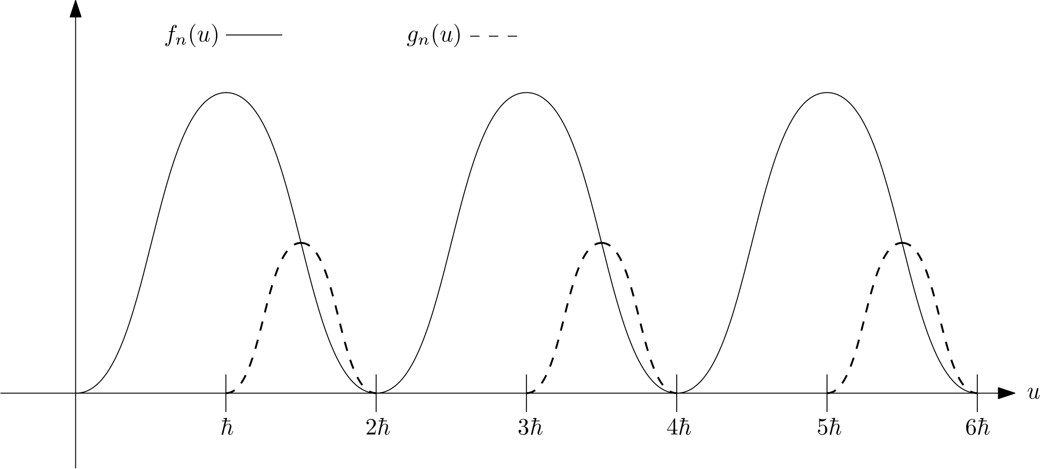 Figure 1
Peer Reviews
No public reviews on file for this paper yet. If you reviewed it on a platform where reviews are public (OpenReview, ICLR, NeurIPS, ICML), you can paste yours below so the community can read it here.
Videos
No videos yet. Explain this paper in a talk, walkthrough, or lecture? Add one.
Projections, modules and connections
for the noncommutative cylinder
Joakim Arnlind and Giovanni Landi
Department of Mathematics
Linköping University
581 83 Linköping
Sweden
Matematica, Università di Trieste
Via A.Valerio, 12/1, 34127 Trieste, Italy
Institute for Geometry and Physics (IGAP) Trieste, Italy
and INFN, Trieste, Italy
(Date: August 2020)
Abstract.
We initiate a study of projections and modules over a noncommutative cylinder, a simple example of a noncompact noncommutative manifold. Since its algebraic structure turns out to have many similarities with the noncommutative torus, one can develop several concepts in a close analogy with the latter. In particular, we exhibit a countable number of nontrivial projections in the algebra of the noncommutative cylinder itself, and show that they provide concrete representatives for each class in the corresponding group. We also construct a class of bimodules endowed with connections of constant curvature. Furthermore, with the noncommutative cylinder considered from the perspective of pseudo-Riemannian calculi, we derive an explicit expression for the Levi-Civita connection and compute the Gaussian curvature.
Contents
1. Introduction
In the rapidly developing and conceptually growing field of noncommutative geometry it has been of paramount importance to have at least one tractable example exhibiting many of the nontrivial subtleties of the theory. In this respect, the noncommutative torus is perhaps the most studied object in noncommutative geometry, and it has served as a inspirational source (as well as testing ground) for many results and concepts in more general situations. However, to explore the notion of noncompact manifolds, the torus is not equally well suited.
In this paper, we set out to study the noncommutative cylinder as a simple manageable example of a noncompact noncommutative manifold which still exhibits nontrivial features. Inspired by the algebraic similarities with the torus, we follow the same lines of thought in order to see to what extent known concepts apply in this noncompact situation as well.
Starting from a known description in terms of Fourier transforms, we choose a particular presentation of the noncommutative cylinder and introduce a (commuting) set of hermitian derivations as well as a trace. After providing basic results about these structures, we proceed to construct a class of projections in the algebra itself, and show that they are classified by the integers. Moreover, by showing that the corresponding projective modules respect the group structure of the integers, we conclude that these projections provide concrete representatives for each class in the group of the noncommutative cylinder (which is known to be ). A corresponding “Chern number” can be computed for each projective module by evaluating the projections against a cyclic 2-cocycle.
Next, in analogy with the torus modules defined by Connes and Rieffel [Con80, Rie81], we find a class of bimodules for the noncommutative cylinder, on which connections of constant curvature are defined. Interestingly, these modules turn out to be isomorphic to copies of the algebra itself. Although the details of the bimodule structure depend on a choice of parameters, it is the case that the curvature only depends on the deformation parameters and defining the left and right algebras, respectively.
Finally, we recall the framework of pseudo-Riemannian calculi, and show that for a given choice of metric, there exists a calculus over the noncommutative cylinder with a unique torsion-free and metric connection, for which one may explicitly compute the Gaussian curvature. Moreover, we illustrate a Gauss-Bonnet type theorem where the total curvature (that is, the integral of the Gaussian curvature with respect to the Riemannian volume form) is shown to be independent of a class of metric perturbations.
2. The algebra of the noncommutative cylinder
Let us start by recalling the definition of the algebra of the noncommutative cylinder. Let denote the space of Schwartz functions on . Every may be written as
[TABLE]
with and we introduce the Fourier transform of the coefficients as
[TABLE]
Thus any function as in (2.1), is written as
[TABLE]
Following the general strategy of [Rie93], we define a twisted convolution product on via
[TABLE]
where , and is a cocycle fulfilling the condition
[TABLE]
ensuring associativity of the product. For our purposes we choose a particular cocycle given by
[TABLE]
Note that this cocycle is cohomologous to its antisymmetrization
[TABLE]
giving the corresponding twisted convolution as defined in [vS04]; the two corresponding algebras are thus isomorphic.
Definition 2.1**.**
Let be the algebra defined by the vector space together with the product in (2.2) for the cocycle
[TABLE]
As the product in is defined on the level of Fourier transforms, let us derive a more explicit expression in the following form.
Proposition 2.2**.**
Let be such that
[TABLE]
Then
[TABLE]
Proof.
The proof consists of a straight-forward computation:
[TABLE]
From Proposition 2.2 one infers the simple commutation rule
[TABLE]
which we shall often use in the following. To slightly simplify the notation, let us introduce such that every may be written as
[TABLE]
In particular, (2.4) now reads
[TABLE]
Remark 2.3*.*
As a side remark, we note that the relation (2.4) can formally be derived from the canonical commutation relation via
[TABLE]
which is in close analogy with the noncommutative catenoid defined in [AH18].
One may readily introduce a -algebra structure on .
Proposition 2.4**.**
For , set
[TABLE]
Then it follows that and .
Proof.
Just compute
[TABLE]
Next, consider
[TABLE]
and compute
[TABLE]
which proves the second statement. ∎
Thus, with respect to the involution defined in Proposition 2.4 the algebra is a -algebra. By representing as multiplication operators on , i.e. for , one may complete in the operator norm to a -algebra which we shall denote by (cf. [vS04]).
Next, let us introduce a set of commuting derivations.
Proposition 2.5**.**
For with
[TABLE]
define
[TABLE]
Then and are hermitian derivations of such that .
Proof.
It is clear that and are linear maps; let us show that they satisfy Leibniz rule. One obtains
[TABLE]
and
[TABLE]
showing that are indeed derivations of . Furthermore, it is easy to see that
[TABLE]
Finally, let us show that and are hermitian derivations. One computes
[TABLE]
as well as
[TABLE]
which proves that are hermitian. ∎
Remark 2.6*.*
Clearly the function is not in the algebra . In spite of this a direct computation shows that one can formally obtain a commutation expression for the derivation , that is
[TABLE]
for any .
On the algebra we have a trace as well.
Definition 2.7**.**
For with
[TABLE]
we set
[TABLE]
It is clear from the definition that is a linear map.
Proposition 2.8**.**
The map is a positive invariant trace; that is, it has the properties
- (1)
, 2. (2)
, 3. (3)
, 4. (4)
,
for all .
Proof.
It is immediate to see that . A direct computation yields
[TABLE]
Furthermore, one finds that
[TABLE]
as well as
[TABLE]
Finally, we check that
[TABLE]
which completes the proof of the statements. ∎
From now on we shall drop the cumbersome notation and simply write when no confusion can arise.
For the noncommutative torus, there exists a convenient cyclic 2-cocycle which can be evaluated on 2-forms. For the noncommutative cylinder, one can make use of a similar construction. The cyclic 2-cocycle below will be used in the next section in order to compute “Chern numbers” of a class of projective modules.
Proposition 2.9**.**
For we set
[TABLE]
Then is a cyclic,
[TABLE]
Hochschild 2-cocycle,
[TABLE]
for all .
Proof.
Let us first show that is cyclic. By using one finds that
[TABLE]
and since (by Proposition 2.8) it follows that
[TABLE]
since . To show that is a cocycle, i.e.
[TABLE]
is a straight-forward computation where one expands all derivatives of products of functions, and uses the fact that . ∎
3. Projections in the algebra
For the noncommutative torus, it is well known that its algebra, in contrast to the commutative case, contains nontrivial projections which one may explicitly describe [Rie81]. In this section, we will show that a similar construction can be carried out for the noncommutative cylinder. Namely, we shall construct projections of the following form:
[TABLE]
Proposition 3.1**.**
Let be real-valued functions, and set
[TABLE]
Then . Moreover if the functions and satisfy
[TABLE]
for all .
Proof.
Since and are real-valued, using (2.5) one immediately obtains
[TABLE]
Then, a straight-forward computation of gives
[TABLE]
which indeed equals by using (3.1)–(3.3). ∎
Let us now construct a particular class of projections satisfying the requirements of Proposition 3.1. Let be a function increasing smoothly from [math] to on the interval , and define as
[TABLE]
Next, for we set
[TABLE]
resulting in shifted copies of the original functions, as depicted in Figure 1. Note that and have compact support being defined on , where they are -periodic by construction.
It is straightforward to check that and satisfy (3.1), (3.2) and (3.3). For instance, for it is immediate that (3.1) and (3.2) holds since . Moreover,
[TABLE]
showing that (3.3) is satisfied as well. Thus, one may conclude from Proposition 3.1 that
[TABLE]
is indeed a projection in . Next, let us compute the trace of these projections.
Proposition 3.2**.**
Let be defined as above. Then .
Proof.
Since is supported on , where it is -periodic, it follows that
[TABLE]
and from the definition of one obtains
[TABLE]
∎
The curvature 2-form related to the projection is given by , which may be evaluated against the cyclic 2-cocycle defined in Proposition 2.9.
Proposition 3.3**.**
For any projection as in (3.6), one has
[TABLE]
Proof.
As
[TABLE]
we compute
[TABLE]
Writing
[TABLE]
one finds that
[TABLE]
giving
[TABLE]
Since for all and for all for ,
[TABLE]
and it follows that
[TABLE]
Noting that for
[TABLE]
one computes
[TABLE]
which proves the statement. ∎
Considering the construction of the projection , and the results in Proposition 3.2 and Proposition 3.3, it is natural to ask how the direct sum of the projective modules defined by and is related to the module defined by . The next result shows that they are indeed isomorphic.
Proposition 3.4**.**
Let be integers with . Then
[TABLE]
as (right) -modules.
Proof.
Let and be given as
[TABLE]
and introduce
[TABLE]
Since is unitarily equivalent to , the modules and are isomorphic and, furthermore, it is clear that . Next, let us show that and are orthogonal; i.e. that . Introduce
[TABLE]
and note that
[TABLE]
since and are disjoint. Using these facts, one finds that
[TABLE]
First of all, it is clear that and since whenever . Furthermore, it also follows that and since for . Thus, we conclude that . For orthogonal projections,
[TABLE]
and in combination with the previous arguments one obtains
[TABLE]
which proves the desired result. ∎
Let us discuss these results from the perspective of -theory. In [vS04], of the noncommutative cylinder was shown to be isomorphic to . Since the algebra is nonunital, one then expects that there exists a countable class of nontrivial projections . In this section we have constructed projections (for each ), and Proposition 3.2 shows that if then and are not equivalent. Moreover, from Proposition 3.4 it follows that the map respects the group structure of the integers, and we conclude that represents the class labeled by . In this sense, one may consider the projection to be a generator of .
4. Bimodules
We now construct -modules on the space of Schwartz functions in one discrete and one real variable in analogy with the noncommutative torus. We show that one may construct left and right -modules, as well as bimodules, depending on a set of parameters. Furthermore, it turns out that these modules are in fact isomorphic to a number of copies of the algebra itself. To begin with, for set
[TABLE]
The corresponding left module structure is given in the following result.
Proposition 4.1**.**
*Let and be such that .
For set*
[TABLE]
for . Then is a left -module such that
[TABLE]
for all .
Proof.
In order for (4.1) to define a module action, one has to check that it respects the relations in the algebra; i.e. \big{(}(fg)\xi\big{)}(x,k)=\big{(}f(g\xi)\big{)}(x,k). One finds that
[TABLE]
by using that . On the other hand
[TABLE]
which is seen to equal \big{(}f(g\xi)\big{)}(x,k). Next, let us show that by first computing
[TABLE]
Let us compare this with
[TABLE]
Setting gives
[TABLE]
and changing the integration variable to yields
[TABLE]
Finally, we set and use that to obtain
[TABLE]
which equals . ∎
In the same way, one may construct a right module structure on . The proof is analogous to that of Proposition 4.1.
Proposition 4.2**.**
*Let and such that .
For set*
[TABLE]
for . Then is a right -module such that
[TABLE]
for all .
A (left or right) -module constructed as above will be denoted by with a suitable choice of parameters implicitly assumed. If the parameters of the left and right module structures are compatible, becomes a -bimodule.
Proposition 4.3**.**
Let and such that
[TABLE]
Then is a -bimodule with respect to the left and right actions defined in Proposition 4.1 and Proposition 4.2.
Proof.
In order for to be a -bimodule, it must hold that
[TABLE]
for all , and . One finds that
[TABLE]
by using that . On the other hand
[TABLE]
since . We conclude that \big{(}g(\xi f)\big{)}(x,k)=\big{(}(g\xi)f\big{)}(x,k). ∎
A bimodule defined as in Proposition 4.3 will be denoted by , again tacitly assuming a choice of the parameters and satisfying the requirements in Proposition 4.3. Note that one can construct bimodules for arbitrary choices of by choosing e.g. such that and setting
[TABLE]
Let us now point out some obvious isomorphisms between modules defined by different sets of parameters. To simplify the description, we make the following definition.
Definition 4.4**.**
The vectors and are called [math]-compatible if either or for .
Proposition 4.5**.**
Let and be left -modules (as in Proposition 4.1) defined by the parameters and , respectively. If and are [math]-compatible then as left -modules.
Proof.
Note that since , it follows that . We shall proceed by defining module homomorphisms as
[TABLE]
for . Note that is a linear map and if then is invertible. Now, let us derive conditions for to be a module homomorphism; thus, we demand that for all . To this end one computes
[TABLE]
The above expressions are equal if
[TABLE]
Note that since and are [math]-compatible, either both sides of each equation are zero (i.e. trivially giving a solution) or both sides are non-zero (as long as ). Thus, if and , then is an isomorphism for any . If and , one can set , solving (4.3) (and similarly in the case when but ). Now, for the case when one sets and notes that
[TABLE]
giving a solution of (4.3). Thus, it follows that under the assumptions given in the proposition, there exists a module isomorphism . ∎
Somewhat surprisingly, it turns out that these modules are in fact isomorphic (as modules) to copies of the algebra itself. More precisely, we formulate the statement as follows.
Proposition 4.6**.**
Let be a left -module defined by the parameters such that and . For arbitrary (considered as a left -module) we write with for , and introduce the components via
[TABLE]
Furthermore, for an integer we let and be defined by . Then the map \phi:\big{(}\mathcal{C}_{\hbar}^{\infty}\big{)}^{r}\to\mathcal{E}_{\hbar}, defined as
[TABLE]
is an isomorphism of left -modules.
Proof.
First of all, it is clear that . Furthermore, one finds that
[TABLE]
as well as
[TABLE]
by using that . Hence, is a left module homomorphism. One may readily construct the inverse
[TABLE]
and check that
[TABLE]
We conclude that is indeed a left module isomorphism. ∎
In the case when and, moreover, is a -bimodule, one can strengthen the result to obtain a bimodule isomorphism.
Proposition 4.7**.**
For , let be a -bimodule (as in Proposition 4.3) with and . The map , defined as
[TABLE]
for , is a bimodule isomorphism with inverse
[TABLE]
for .
Proof.
The fact that is a left module isomorphism with
[TABLE]
follows immediately from Proposition 4.6 (and its proof). Before showing that is a also a right -module homomorphism, let us derive a few properties of the parameters defining the module. For a bimodule with and one necessarily has (otherwise implying ). Hence, one may solve for and to obtain
[TABLE]
and we note that
[TABLE]
Now, one computes for
[TABLE]
and
[TABLE]
since . Moreover, changing the summation index to gives
[TABLE]
by using that and , as shown in (4.5). ∎
4.1. Hermitian structures
Continuing the analogy with the noncommutative torus, we show there exist hermitian structures on the -bimodule .
Proposition 4.8**.**
Let be a -bimodule, as in Proposition 4.3, and define and as
[TABLE]
Then it follows that
[TABLE]
as well as the compatibility condition
[TABLE]
for , and .
Remark 4.9*.*
Strictly speaking, is not defined since does not decay as (and, hence, does not belong to the algebra). However, having in mind the left action (4.1), we interpret the above expression as
[TABLE]
and allow ourselves a formulation as in Proposition 4.8 since it more clearly reflects the idea behind the construction. Similarly for the right structure.
Proof.
Let us start by showing that . Thus, we set
[TABLE]
and write
[TABLE]
Now, let us replace by its Fourier integral:
[TABLE]
By a change of variables we set and , giving
[TABLE]
The proof of the statement is completely analogous. Finally, we need to show compatibility of the two products; namely, that
[TABLE]
for . One writes
[TABLE]
A similar computation for gives
[TABLE]
To prove that the expressions for and \big{(}\xi\langle\eta,\psi\rangle_{\bullet}\big{)}(x,k) are equal for all and , we compare the sums term by term. Let us proceed as follows: We fix arbitrary in the expression for and arbitrary in the expression for \big{(}\xi\langle\eta,\psi\rangle_{\bullet}\big{)}(x,k). Now, for every such choice we will prove that there exists and such that the corresponding terms are equal. Setting
[TABLE]
one finds (by comparing the arguments of , and ) that the corresponding terms in the two sums are equal if
[TABLE]
Inserting and into these equations yields
[TABLE]
as the remaining conditions. However, these conditions are true due to the fact that is assumed to be a bimodule fulfilling the requirements of Proposition 4.3. ∎
4.2. Bimodule connections
Let us now turn to the question of finding connections on the bimodule , of the form
[TABLE]
for , and we start by working out the conditions for to be a left connection; that is, such that
[TABLE]
for , and .
Proposition 4.10**.**
Let be a left -module with respect to a choice of (as in Proposition 4.1) with . If and then , as defined in (4.6), is a left module connection.
Proof.
One finds that
[TABLE]
since . Furthermore,
[TABLE]
since , showing that is a left module connection. ∎
Remark 4.11*.*
By using the isomorphism in (4.4) one may induce connections on the algebra itself via
[TABLE]
for , giving
[TABLE]
and
[TABLE]
using the expression (2.6) for .
It is straightforward to compute the curvature of in (4.6):
[TABLE]
showing that has a constant curvature equal to . Note that the curvature does not depend on , which implies that one may construct connections with arbitrary constant curvature. Namely, let and set
[TABLE]
clearly fulfilling the requirements of Proposition 4.10, giving a connection of constant curvature .
Moreover, one easily shows that the curvature is -linear, that is
[TABLE]
for and , implying that the curvature is an element of
[TABLE]
for and ; this is an algebra under composition.
Given a left connection on , one can define associated derivations on from the commutators
[TABLE]
for and . If is also a right -module, then (acting on the right) is a subalgebra of . On the algebra , with the connection as in (4.6) one recovers a rescaling of the natural derivations from (4.7), as stated in the following result.
Proposition 4.12**.**
Let be a -bimodule with and let be a left module connection as defined in (4.6). Then on the derivations in (4.7) are given by
[TABLE]
Proof.
With the right structure as in (4.2), one computes
[TABLE]
as well as
[TABLE]
which establish the results. ∎
As a corollary we have the condition for to be a right module connection.
Proposition 4.13**.**
Let be a -bimodule with and let be a left module connection as defined in (4.6). If and then is a right module connection; that is,
[TABLE]
for , and .
Proof.
With the restriction on the parameters one has for and . With (acting on the right), (4.7) becomes
[TABLE]
showing that is indeed a (right) connection. ∎
In order for to be a bimodule connection on the parameters, apart from satisfying the requirements of a bimodule, need to satisfy the requirements of Proposition 4.10 and Proposition 4.13. Let us work out what this implies for the parameters.
Proposition 4.14**.**
For and , let be a -bimodule with parameters and respectively, satisfying the requirements of Proposition 4.3, and assume that are such that
[TABLE]
- (1)
If then , , and
[TABLE] 2. (2)
If then and
[TABLE]
Proof.
The requirements on the parameters can be summarized as:
[TABLE]
and we note that (4.8) and (4.11) imply , and (4.9) and (4.10) imply that , giving
[TABLE]
Let us first consider the case when , which implies by (4.13) that or . However, if then (4.8) and (4.11) imply that , which contradicts the assumption that . Hence, one must have that . Next, we note that since otherwise (4.8) and (4.11) imply that . The same kind argument shows that if (otherwise (4.8) and (4.9) imply that ). Thus, the following equations remain to be solved:
[TABLE]
The last equation implies that which gives since . Solving the above system for the variables immediately gives the claimed result.
Next, let us consider the case when . Equation (4.13) then implies that and , giving
[TABLE]
Equations (4.8) and (4.11) imply that which, by inserting the above expression, gives
[TABLE]
which in particular implies that . With and , (4.8)–(4.12) are equivalent to
[TABLE]
Solving the first to equations for gives
[TABLE]
which, furthermore, gives
[TABLE]
Inserting the expression for into gives
[TABLE]
(using ) and finally
[TABLE]
completing the proof. ∎
Thus, if then which implies that a -bimodule connection of the type (4.6) has zero curvature
[TABLE]
In the situation when , Proposition 4.14 shows that in order for such a bimodule connection to exist, the ratio between and has to be rational (note that, they need not themselves be rational). Moreover, in this case one may always find module parameters guaranteeing that is a bimodule connection. The curvature then becomes
[TABLE]
It is noteworthy that the curvature is independent of the particular parameters defining the bimodule structure, since it only depends on and . Moreover, since is rational from (4.14), the curvature is a rational multiple of .
5. A pseudo-Riemannian calculus
In [AW17a, AW17b] the concept of pseudo-Riemannian calculi was introduced in order to discuss Levi-Civita connections on vector bundles over noncommutative manifolds. In this particular setting, one can prove that there exists at most one metric and torsion-free connection on a vector bundle which is equipped with a soldering map; that is a linear map which maps derivations into sections of the bundle. In this section, we shall construct a pseudo-Riemannian calculus for the noncommutative cylinder and explicitly compute the Levi-Civita connection as well as the corresponding curvature.
We recall a few definitions. For the time being, we assume that is an arbitrary -algebra.
Definition 5.1**.**
Let be a (right) -module and let be a non-degenerate -valued hermitian form on . Furthermore, let be a real Lie algebra of hermitian derivations of and let be a -linear map. The data is called a real metric calculus over if
- (1)
the image generates as an -module, 2. (2)
for all .
An affine connection on is a map such that (with the notation ), one has
- (1)
, 2. (2)
, 3. (3)
\nabla_{\partial}(Ua)=\big{(}\nabla_{\partial}U\big{)}a+U\partial(a),
for all , , and .
Definition 5.2**.**
Let be a real metric calculus and let denote an affine connection on . If
[TABLE]
for all and then is called a real connection calculus.
Definition 5.3**.**
Let be a real connection calculus over . The calculus is metric if
[TABLE]
for all , , and torsion-free if
[TABLE]
for all . A metric and torsion-free real connection calculus over is called a pseudo-Riemannian calculus over .
Within this framework, the uniqueness of a metric and torsion-free connection can be stated in the following way.
Theorem 5.4** ([AW17b]).**
Let be a real metric calculus over . Then there exists at most one affine connection on , such that is a pseudo-Riemannian calculus.
Let us now return to the noncommutative cylinder. The algebra consists of smooth functions on that fall off rapidly at infinity. Of course, there are many more smooth functions on and in this section we allow ourselves to consider a different algebra consisting of elements
[TABLE]
where is such that only for a finite number of terms. The product is defined as before as
[TABLE]
and the -algebra structure is again given as in Proposition 2.4. Note that whenever the products of the two algebras coincide (as well as the involution). In what follows, we shall construct a pseudo-Riemannian calculus over .
Let denote the real (abelian) Lie algebra generated by the hermitian derivations , and let denote the free (right) -module of rank 2, with basis . Moreover, we introduce the hermitian form
[TABLE]
for and and such that . (Here and in the following we sum over up-down repeated indices from 1 to 2.) We shall assume that is invertible in the sense that there exists such that . (For instance, one might choose for arbitrary (real) .) Clearly, is nondegenerate in the sense that for all implies that .
Finally, we define as (for ) extended linearly to all of . It is immediate that the image of generate and that is hermitian for all in the image of . These considerations imply that is a real metric calculus over . The (unique) Levi-Civita connection can be computed via Koszul’s formula (cf. [AW17a, AW17b]) which, since , becomes
[TABLE]
where . Writing gives
[TABLE]
and one finds that
[TABLE]
Let us exemplify this construction for . In this case, one obtains
[TABLE]
giving
[TABLE]
We immediately note that
[TABLE]
since both and depend only on . This implies that the curvature of the connection will have all the classical symmetries [AW17b]; hence, there is only one independent component of the curvature, and one finds
[TABLE]
giving the Gaussian curvature as
[TABLE]
For a metric of the above form, a natural integration measure corresponding to the volume form is given by . For the sake of illustration, let us compute the total curvature (when it exists)
[TABLE]
Here one notes a certain independence of the total curvature with respect to perturbations of the metric; i.e. for one finds that whenever
[TABLE]
For instance, for , corresponding to the induced metric on the catenoid (cf. [AH18]), one obtains
[TABLE]
which, in the geometrical situation where the trace naturally gains a factor of (from the integration along ), gives the expected value of for the total curvature of the catenoid.
Acknowledgments
JA is supported by the Swedish Research Council. GL is partially supported by INFN, Iniziativa Specifica “Gauge and String Theories (GAST)”, and by the “National Group for Algebraic and Geometric Structures and their Applications (GNSAGA - INdAM)”, and “Laboratorio Ypatia di Scienze Matematiche (LIA-LYSM)” CNRS - INdAM.
The reference list from the paper itself. Each links out to its DOI / PubMed record.
- 1[AH 18] J. Arnlind and C. Holm, A noncommutative catenoid , Lett. Math. Phys. 108 (2018), no. 7, 1601–1622.
- 2[AW 17a] J. Arnlind and M. Wilson, On the Chern-Gauss-Bonnet theorem for the noncommutative 4 4 4 -sphere , J. Geom. Phys. 111 (2017), 126–141.
- 3[AW 17b] J. Arnlind and M. Wilson, Riemannian curvature of the noncommutative 3 3 3 -sphere , J. Noncommut. Geom. 11 (2017), no. 2, 507–536.
- 4[Con 80] A. Connes, C ∗ superscript 𝐶 ∗ C^{\ast} algèbres et géométrie différentielle , C. R. Acad. Sci. Paris Sér. A-B 290 (1980), no. 13, A 599–A 604.
- 5[Rie 81] M.A. Rieffel, C ∗ superscript 𝐶 ∗ C^{\ast} -algebras associated with irrational rotations , Pacific J. Math. 93 (1981), no. 2, 415–429.
- 6[Rie 93] M.A. Rieffel, Deformation quantization for actions of 𝐑 d superscript 𝐑 𝑑 {\bf R}^{d} , Mem. Amer. Math. Soc. 106 (1993), no. 506, x+93.
- 7[v S 04] W.D. van Suijlekom, The noncommutative Lorentzian cylinder as an isospectral deformation , J. Math. Phys. 45 (2004), no. 1, 537–556.