Computing wedge probabilities: finite time horizon case
Dmitry Muravey

TL;DR
This paper introduces an alternative infinite series formula for computing the probability that a Brownian motion stays within sloping boundaries over a finite time, offering faster convergence and high precision.
Contribution
It provides a new series representation for wedge probabilities with improved convergence properties and practical rules for choosing the optimal formula based on parameters.
Findings
Convergence rate depends on boundary slopes and time.
Six terms of the series achieve precision of 10^{-16}.
The new formula offers an efficient alternative to Anderson's formula.
Abstract
We present an alternative to the well-known Anderson's formula for the probability that a first exit time from the planar region between two slopping lines -a_1 t -b_1 and a_2 t + b_2 by a standard Brownian motion is greater than T. As the Anderson's formula, our representation is an infinite series from special functions. We show that convergence rate of both formulas depends only on terms (a_1 + a_2)(b_1 + b_2) and (b_1 + b_2)^2 /T and deduce simple rules of appropriate representation's choose. We prove that for any given set of parameters a_1, b_1, a_2, b_2, T the sum of first 6 terms ensures precision 10^{-16}.
Click any figure to enlarge with its caption.
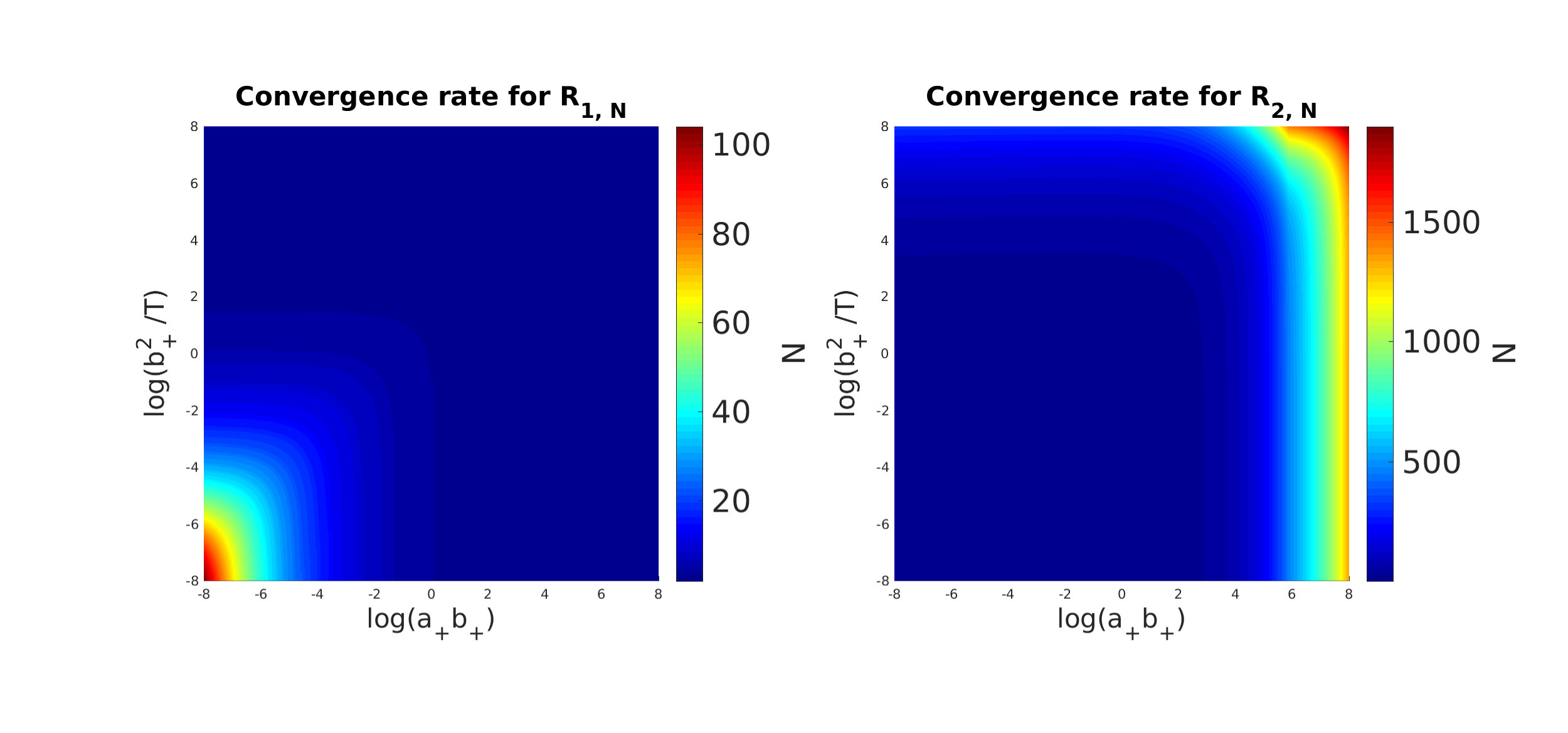 Figure 1
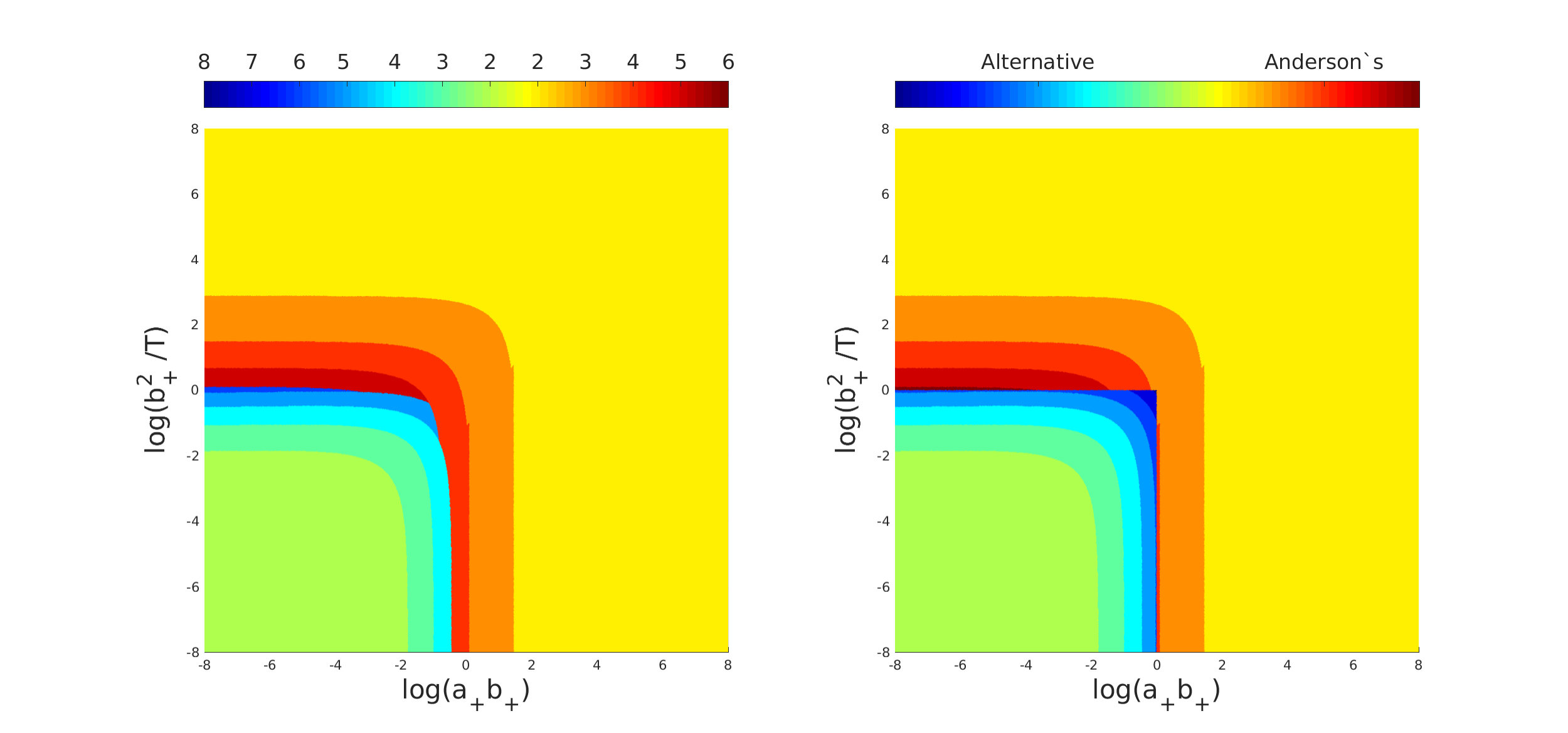 Figure 2
Peer Reviews
No public reviews on file for this paper yet. If you reviewed it on a platform where reviews are public (OpenReview, ICLR, NeurIPS, ICML), you can paste yours below so the community can read it here.
Videos
No videos yet. Explain this paper in a talk, walkthrough, or lecture? Add one.
Taxonomy
TopicsBayesian Methods and Mixture Models · Data Management and Algorithms · Soil Geostatistics and Mapping
Computing wedge probabilities: finite time horizon case
Dmitry Muravey111e-mail:[email protected].
Abstract
We present an alternative to the well-known Anderson’s formula for the probability that a first exit time from the planar region between two slopping lines and by a standard Brownian motion is greater than . As the Anderson’s formula, our representation is an infinite series from special functions. We show that convergence rate of both formulas depends only on terms and and deduce simple rules of appropriate representation’s choose. We prove that for any given set of parameters , , , , the sum of first 6 terms ensures precision .
Contents
1 Introduction
Let be a standard Brownian motion. We consider the following exit times
[TABLE]
where process is defined as . Let’s denote by probability conditional on the process started at . We omit subscript if process starts at zero, i.e. if is a standard Brownian motion. The probability is called wedge probability and have been studied by many authors [2], [3]. Anderson [2] was the first to obtain the explicit representation for the in terms of infinite series from normal c.d.f. functions. The explicit formula for was found by Doob [4]. Based on properties of Jacobi theta functions, Ycart and Drouilhet [6] have found alternative to Doob’s formula. They also computed uniform precision estimates and proposed efficient numerical algorithm. Let us mention that connection of with theta functions has been pointed out by Salminen and Yor [5].
In this paper we generalize results from [6] to the finite time horizon case. Based on Lie symmetries for the heat equation, we deduce alternative to Anderson’s formula. Our representation is an infinite series from Error functions with complex argument. For numerical computations we derive another representation containing only real functions. Combining our results with Anderson’ formula we propose simple numerical algorithm for computation of . We show that convergence rate of these two series depends only on two terms: and . Anderson’ formula converges fast if at least one term is relatively high, our formula has fast convergence for the opposite case. The algorithmic consequence is that computing at most six terms of the series either in Anderson’s formula or in the new alternative suffices to approximate with precision smaller than .
The rest of paper is organized by the following scheme: in Section 2 we show connections of with in terms of corresponded PDE boundary-value problems. Based on Lie symmetries for the heat equation we derive the solutions of these PDEs in explicit form. Section 3 contains explicit formulas for probability . We re-derive famous Anderson’s formula and present two new representations. Also we show that Doob’s and Ycart and Drouilhet’ formulas can be derived as the limiting form . In the last Section 4 we present upper bounds for the remainders of infinite series from Anderson’ formula and its alternative. Based on these results, we deduce rules describing in which cases Anderson’s formula or its alternative should be used and propose simple numerical algorithm for computation of wedge probability .
2 PDE and Lie symmetries approach to analysis of stopping times and
From standard results in probability theory and can be represented in the following form
[TABLE]
Functions and solve the following Cauchy problems with killed boundary conditions for Fokker–Planck–Kolmogorov equation:
[TABLE]
Here is the adjoint of , which is the infinitesimal generator of the process . In case of standard Brownian motion operator is self-adjoint, i.e.
[TABLE]
Initial condition is a Dirac measure at the point . In the next Proposition we present explicit formulas for .
Proposition 1**.**
Function has two equivalent representations ():
[TABLE]
Proof.
First formula can be derived from the following well-known representation
[TABLE]
The phase shift and frequencies are set to satisfy boundary conditions , i.e, , and . Hence at the moment function is Fourier series on the segment . Calculation of coefficients turns out to the main formula (4).
Second formula in (4) can be obtained by using of Laplace transform with respect to the time variable . This integral transform reduces original initial boundary problem to the simple boundary problem for linear ODE:
[TABLE]
Here is an image of transformation, i.e.
[TABLE]
The problem (8) can be easily solved by a standard techniques. Inversion of Laplace transform yields second formula (4). ∎
Remark 1**.**
We can also derive identity between two representations from (4) by using Poisson’ summation formula
[TABLE]
In he next proposition we establish connection of with .
Proposition 2**.**
Function can be explicitly represented in terms of :
[TABLE]
here constants , and are equal
[TABLE]
Proof.
This fact follows from Lie symmetries for the heat equation. One can check by the direct calculations that function from (9) solves equation . Note that function is equal to zero if or , therefore equals zero if solves one of the following equations:
[TABLE]
Hence the boundary conditions are satisfied. Now we check the initial condition :
[TABLE]
∎
3 Explicit formulas for wedge probability
3.1 Some auxiliary functions and terms
Let’s define the following function :
[TABLE]
and recall well known Error function and normal c.d.f. :
[TABLE]
Function can be represented in terms of and
[TABLE]
Let us note that function also has the following properties:
[TABLE]
3.2 Explicit formulas for wedge probability
We will use the following notations for wedge probabilities and :
[TABLE]
Proposition 3** (Anderson).**
Wedge probability has the following representation:
[TABLE]
Here are defined by the following formulas:
[TABLE]
and function is defined in (11).
Proof.
Employ identity
[TABLE]
in the (9) and choose the first formula for from (4) with .
[TABLE]
Here
[TABLE]
One can check that
[TABLE]
and
[TABLE]
In the result we have
[TABLE]
Rearrangement of the first and second sum
[TABLE]
yields formula (16). It is easy to check that (see also [6])
[TABLE]
∎
Remark 2**.**
Doob’ formula
[TABLE]
can be easily derived from (16) if we tends . Note that if and have opposite signs then .
Proposition 4**.**
Formula (16) has the following alternatives:
[TABLE]
or
[TABLE]
Here function is defined in (11).
Proof.
From Propositions 1 and 2 we have the following formula for :
[TABLE]
Change of integration variable yields formula (22). Definite integral from (22) is known (see [1]) and can be expressed in terms of Error functions (from complex argument):
[TABLE]
or (see (13))
[TABLE]
Using the last formula in (22) and changing the sign of in the second term gives the representation (21). ∎
Remark 3**.**
Ycart and Drouilhet formula can be derived from (21) by :
[TABLE]
Here is defined as (see [6]).
4 Computational aspects
4.1 Convergence rates
Proposition 5**.**
Let’s denote by and the partial sums in series (16) and (22) respectively and consider the remainders:
[TABLE]
For :
[TABLE]
Proof.
At first we note that , , , are larger than (see [6]) and apply second property of function from (14):
[TABLE]
If quantity is sufficiently large, then we can use Ycart and Drouilhet bounds [6] (this is second line in formula (25)) for the remainder . If this term is sufficiently small, then we derive upper bound in the assumption .
Now we show that for any the arguments of any function from the formula above are positive:
[TABLE]
for the second and third line:
[TABLE]
and for fourth line we apply the following inequality:
[TABLE]
Therefore,
[TABLE]
Application of the following inequality
[TABLE]
yields the following upper bound for the remainder :
[TABLE]
For the remainder we apply the following bounds:
[TABLE]
∎
In case of the bounds for remainders depend only on . In the finite horizon case we have one extra term . We show that remainders and are characterized only by these terms. Denote by
[TABLE]
and employ these new variables in formulas (25) and (26):
[TABLE]
4.2 Convergence analysis and implementation
In this subsection we present numerical experiments illustrating convergence rates for the series (16) and (22). As we mentioned before, convergence rates depend only on values of and which are defined in (27). Figure 1 illustrates the log-log plot of convergence rates. Color indicates minimal value of such that remainders and are less than . We can see that our formula convergences faster in case of and . In other cases Anderson’s formula converges faster than alternative.
Left sub-figure in 2 illustrates dependencies of minimal value on values of and . Let us mention, that minimal value of is equal to 5 for Anderson’s formula and to 6 for the alternative. Formula (21) should be used in the region defined by the curve which separates blue and red zones (see left Figure 2). Implementation of this rule can be difficult, so we suggest the following rule: we use our formula if and only if and . Values of are presented in right Figure 2. In this case minimal value of is increases up to 8 terms.
We implement our algorithm in C++11. All terms in formula (16) have been coded by using of functions from the standard library (std::exp and std::erf). Computation of definite integral in formula (22) have been implemented by the help of Simpson’ formula. Numerical experiments have been made using vectors of simulated entries with uniform distribution on for , , , and on for . The running time on a standard laptop is approx. 7 seconds for values.
Remark 4**.**
If we rearrange our formula (22) in the manner of Ycart and Drouilhet formula [6, formula 4] (i.e. apply product-to-sum identity for sines), we shall cut in half. Hence, in these terms we have (i.e. is equal to the infinite horizon case) for our formula.
The reference list from the paper itself. Each links out to its DOI / PubMed record.
- 1[1] Abramowitz M., Stegun I. (1972) Handbook of Mathematical Functions with Formulas, Graphs and Mathematical Tables.
- 2[2] Anderson T.W. A modification of sequential probability ration test to reduce sample size. Ann. Math. Statist., 31(1):165-197, 1960.
- 3[3] Barba Escriba L. A stopped Brownian motion formula with two slopping line boundaries. Ann. Probab. , 15(4): 1524–1526, 1987.
- 4[4] Doob J.L. Heuristic approach to the Kolmogorov-Smirnov theorems. Ann. Math. Statist., 20(3):393-403, 1949.
- 5[5] Salminen P., Yor M. On hitting times of affine boundaries by reflecting Brownian motion and Bessel processes. Period. Math. Hungarica , 62(1):75–191, 2011.
- 6[6] Ycart B., Drouilhet R. (2016) Computing wedge probabilities. Preprint https://arxiv.org/pdf/1612.05764 .