Sampled-data Output Regulation of Unstable Well-posed Infinite-dimensional Systems with Constant Reference and Disturbance Signals
Masashi Wakaiki, Hideki Sano

TL;DR
This paper develops a method for designing finite-dimensional sampled-data controllers to achieve output regulation and disturbance rejection in unstable infinite-dimensional systems with constant signals, using Nevanlinna-Pick interpolation.
Contribution
It introduces a sufficient condition for the existence of such controllers and proposes a design approach based on interpolation techniques, extending to systems with delays.
Findings
Finite-dimensional controllers can achieve output regulation for unstable infinite-dimensional systems.
The design method employs Nevanlinna-Pick interpolation with interior and boundary conditions.
Applicable to systems with state and output delays.
Abstract
We study the sample-data control problem of output tracking and disturbance rejection for unstable well-posed linear infinite-dimensional systems with constant reference and disturbance signals. We obtain a sufficient condition for the existence of finite-dimensional sampled-data controllers that are solutions of this control problem. To this end, we study the problem of output tracking and disturbance rejection for infinite-dimensional discrete-time systems and propose a design method of finite-dimensional controllers by using a solution of the Nevanlinna-Pick interpolation problem with both interior and boundary conditions. We apply our results to systems with state and output delays.
Click any figure to enlarge with its caption.
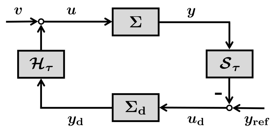 Figure 1
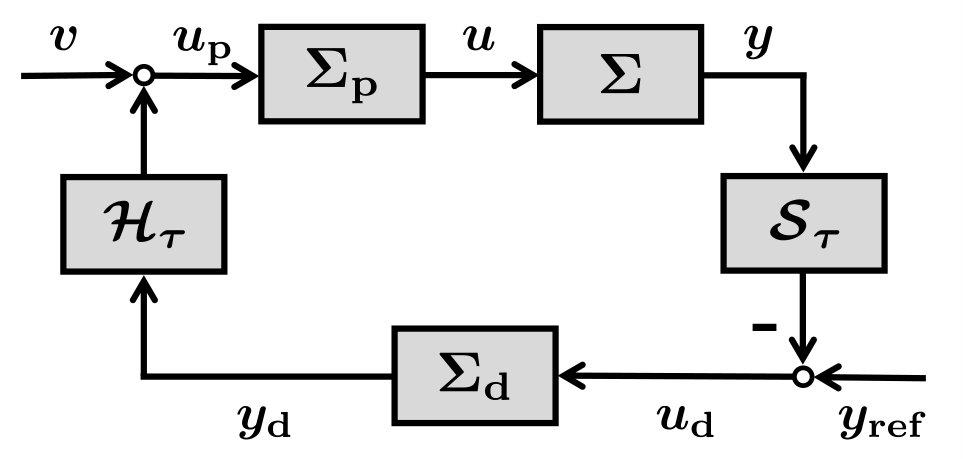 Figure 2
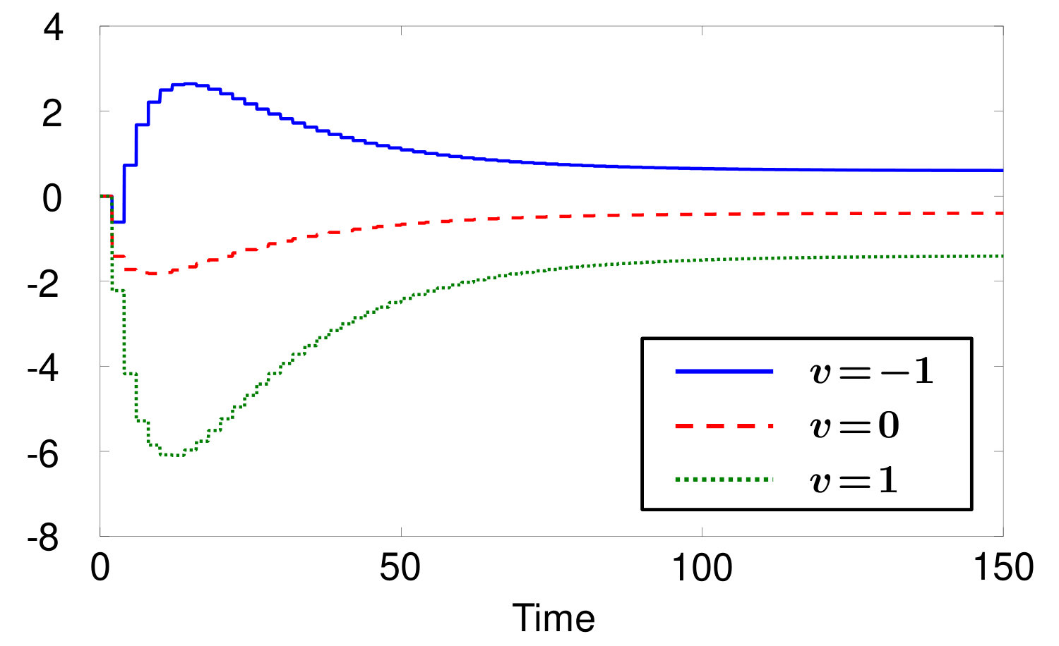 Figure 3
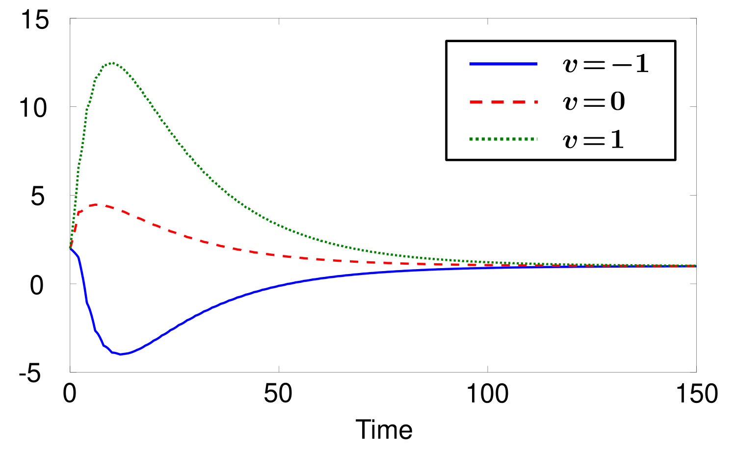 Figure 4
Peer Reviews
No public reviews on file for this paper yet. If you reviewed it on a platform where reviews are public (OpenReview, ICLR, NeurIPS, ICML), you can paste yours below so the community can read it here.
Videos
No videos yet. Explain this paper in a talk, walkthrough, or lecture? Add one.
Taxonomy
TopicsStability and Controllability of Differential Equations · Advanced Mathematical Modeling in Engineering · Nonlinear Differential Equations Analysis
∎
11institutetext: M. Wakaiki 22institutetext: Graduate School of System Informatics, Kobe University, Nada, Kobe, Hyogo 657-8501, Japan
Tel.: +8178-803-6232
Fax: +8178-803-6392
22email: [email protected] 33institutetext: H. Sano 44institutetext: Graduate School of System Informatics, Kobe University, Nada, Kobe, Hyogo 657-8501, Japan
Tel.: +8178-803-6380
Fax: +8178-803-6392
44email: [email protected]
Sampled-data Output Regulation of Unstable Well-posed Infinite-dimensional Systems
with Constant Reference and Disturbance Signals ††thanks: This work was supported by JSPS KAKENHI Grant Numbers JP17K14699.
Masashi Wakaiki
Hideki Sano
(Received: date / Accepted: date)
Abstract
We study the sample-data control problem of output tracking and disturbance rejection for unstable well-posed linear infinite-dimensional systems with constant reference and disturbance signals. We obtain a sufficient condition for the existence of finite-dimensional sampled-data controllers that are solutions of this control problem. To this end, we study the problem of output tracking and disturbance rejection for infinite-dimensional discrete-time systems and propose a design method of finite-dimensional controllers by using a solution of the Nevanlinna-Pick interpolation problem with both interior and boundary conditions. We apply our results to systems with state and output delays.
Keywords:
Frequency-domain methods Output regulation Sampled-data control State-space methods Well-posed infinite-dimensional systems
MSC:
93B52 93C05 93C25 93C35 93C57 93D15
1 Introduction
Due to the development of computer technology, digital controllers are commonly implemented for continuous-time plants. We call such closed-loop systems sampled-data systems. In addition to their practical motivation, sampled-data systems yield theoretically interesting problems related to the combination of both continuous-time and discrete-time dynamics, and various techniques such as the lifting approach Bamieh1992 ; Yamamoto1994 ; Yamamoto1996 and the frequency response operator approach Hagiwara1995 ; Araki1996 have been also developed for the analysis and synthesis of sampled-data finite-dimensional systems. Sampled-data control theory for infinite-dimensional systems has been developed, e.g., in Rebarber1998 ; Rebarber2002 ; Logemann1997 ; Logemann2003 ; Logemann2005 ; Rebarber2006 ; Ke2009SIAM ; Ke2009IEEE ; Ke2009SCL ; Logemann2013 ; Selivanov2017 . Several specifically relevant studies will be cited below again. In this paper, we study the problem of sampled-data output regulation for unstable well-posed systems. The main objective in our control problem is to find finite-dimensional digital controllers achieving the output tracking of given constant reference signals in the presence of external constant disturbances. A theory for well-posed systems has been extensively developed; see, e.g., the survey Weiss2001 ; Tucsnak2014 and the book Staffans2005 . Well-posed systems allow unbounded control and observation operators and provide a framework to formulate control problems for systems governed by partial differential equations with point control and observation and by functional differential equations with delays in the state, input, and output variables.
Our output regulation method is based on the internal model principle, which was originally developed for finite-dimensional systems in Francis1975 and was later generalized for infinite-dimensional systems with finite-dimensional and infinite-dimensional exosystems in Yamamoto1988servo ; Paunonen2010 ; Paunonen2014 ; Paunonen2017TAC ; Paunonen2017SIAM and references therein. In particular, output regulation of nonsmooth periodic signals has been extensively studied as repetitive control hara1988 . For regular systems, which is a subclass of well-posed systems, the authors of Xu2004 ; Paunonen2016TAC ; Paunonen2017SIAM ; Boulite2018 have provided design methods of continuous-time controllers for robust output regulation. For stable well-posed systems with finite-dimensional exosystems, low-gain controllers suggested by the internal model principle have been constructed for the continuous-time setup in Logemann1997SIAM ; Rebarber2003 and for the sampled-data setup in Logemann1997 ; Ke2009SIAM ; Ke2009IEEE ; Ke2009SCL . The difficulty of the problem we consider arises from the instability of well-posed systems. If the system is unstable, then low-gain controllers cannot achieve closed-loop stability. Ukai and Iwazumi Ukai1990 have developed a state-space-based design method of finite-dimensional controllers for output regulation of unstable continuous-time infinite-dimensional systems, by using residue mode filters proposed in Sakawa1983 . On the other hand, we employ a frequency-domain technique based on coprime factorizations as in Logemann1997SIAM ; Logemann1997 ; Hamalainen2000 ; Laakkonen2015 ; Laakkonen2016 . In particular, we extend a design method of stabilizing sampled-data controllers in Logemann2013 to output regulation.
Let and be generating operators and a transfer function of a well-posed system , respectively. The operator is the generator of a strongly continuous semigroup , which governs the dynamics of the system without control. The operators and are control and observation operators, respectively. We consider only infinite-dimensional systems that has finite-dimensional input and output spaces with the same dimension. In other words, the transfer function is a square-matrix-valued function. The well-posed system is connected with a discrete-time linear time-invariant controller through a zero-order hold and a generalized sampler , where is a sampling period. Let be the input and output of the well-posed system and be the input and output of the digital controller , respectively. The generalized sampler is written as
[TABLE]
where the scalar weighting function belongs to and satisfies . In well-posed systems, the output is in , and hence the ideal sampling, i.e., point evaluation does not make sense. The weighting function should be chosen so that the sampled-data system is detectable.
Using the zero-order hold and the generalized sampler , we consider the sampled-data feedback of the form
[TABLE]
where and are constant external reference and disturbance signals, respectively. Fig. 1 illustrates the sampled-data system we study. Since the output of well-posed systems belongs to , the output is not guaranteed to converge to as . In this paper, we therefore consider the convergence of the output in the “energy” sense, i.e., there exist constants and such that
[TABLE]
for all initial states of and of and all , where is the -space weighted by the exponential function . The above condition means that as , the “energy” of the restricted tracking error exponentially converges to zero. If we embed a smoothing precompensator between the plant and the zero-order hold as proposed in Logemann2013 , then the output exponentially converges to in the usual sense under a certain regularity assumption on initial states.
Before studying the sampled-data output regulation problem, we investigate an output regulation problem for infinite-dimensional discrete-time systems. In the discrete-time setup, we propose a design method of finite-dimensional controllers that achieve output regulation. Although in the sampled-data setup, we consider only constant reference and disturbance signals, the proposed method in the discrete-time setup allows reference and disturbance signals that are finite superpositions of sinusoids. The construction of regulating controllers consists of two steps: First we design stabilizing controllers with a free parameter in , using the techniques developed in Logemann1992 ; Logemann2013 . Next we choose the free parameter so that the controller incorporates an internal model for output regulation. The design problem of regulating controllers is reduced to the Nevanlinna-Pick interpolation problem with both interior and boundary conditions. In the reduced interpolation problem, interior conditions are required for stabilization, whereas boundary conditions arise from output tracking and disturbance rejection.
Our main result, Theorem 3.10, states that there exists a finite-dimensional digital controller that achieves output regulation for constant reference and disturbance signals if the following conditions are satisfied:
- (i)
The resolvent set of contains [math]. 2. (ii)
. 3. (iii)
The unstable part of the spectrum of consists of finitely many eigenvalues with finite multiplicities. 4. (iv)
The semigroup generated by the stable part of is exponentially stable. 5. (v)
The unstable part of is controllable and observable. 6. (vi)
For every nonzero integer , does not belong to the spectrum of . 7. (vii)
For every unstable eigenvalues of , . 8. (viii)
For every unstable eigenvalues of and nonzero integer , . 9. (ix)
The multiplicities of all unstable eigenvalues of are one.
The assumptions (iii)– (viii) are used for sampled-data stabilization in Logemann2013 . In fact, (iii)–(vii) are sufficient for the existence of sampled-data stabilizing controllers, and further, (iii)–(viii) are necessary and sufficient in the single-input and single-output case. In particular, (v)–(viii) is used to guarantee that the unstable part of the sampled-data system is controllable and observable. We place the assumptions (i) and (ii) for output regulation. The remaining assumption (ix) is used to reduce the design problem of stabilizing controllers to an interpolation problem of functions in the -space. In the multi-input and multi-output case, the assumption (ix) makes it easy to obtain the associated interpolation conditions. We can remove (ix) in the single-input and single-output case.
The paper is structured as follows. In Section 2, we study an output regulation problem for infinite-dimensional discrete-time systems. In Section 3, we obtain a sufficient condition for the existence of finite-dimensional sampled-data regulating controllers for unstable well-posed systems with constant reference and disturbance signals. In Section 4, we illustrate our results by applying them to systems with state and output delays.
Notation and terminology
We denote by and the set of nonnegative integers and the set of nonnegative real numbers, respectively. For , we define , and for , . We also define and . For a set , its closure is denoted by . For an arbitrary set , the indicator function of is denoted by . For a matrix , let us denote by , , and the conjugate transpose, the matrix with complex conjugate entries, and the adjugate matrix of , respectively.
Let and be Banach spaces. Let denote the space of all bounded linear operators from to . We set . An operator is said to be power stable if there exist and such that for every . Let be a strongly continuous semigroup on . The exponential growth bound of is denoted by , that is, . We say that the strongly continuous semigroup is exponentially stable if . For a linear operator from to , let denote the domain of . The spectrum and resolvent set of a linear operator are denoted by and , respectively.
For , we define the weighted -space by , where for , with the norm . The space of all functions from to is denoted by . Set for every and every . Let , , or . Let denote the space of all bounded holomorphic functions from to . The norm of is given by . We write for .
2 Discrete-time output regulation
In this section, we construct finite-dimensional controllers for the robust output regulation of infinite-dimensional discrete-time systems. Before proceeding to technical details, we describe the overview of this section. A fundamental assumption throughout this paper is that an infinite-dimensional plant can be decomposed into a finite-dimensional unstable part and an infinite-dimensional stable part. To avoid spill-over effects Balas1978 , we cannot ignore the infinite-dimensional stable part completely in the design of stabilizing controllers. However, it has been shown in Logemann1992 ; Logemann2013 that if the infinite-dimensional stable part is appropriately approximated by a finite-dimensional stable system, then we can design finite-dimensional stabilizing controllers. Now one may ask the following question for the problem of output regulation:
By such an approximation-based method, can we always construct stabilizing controllers that incorporate an internal model?
To stabilize the plant, the approximation error should be small. However, it is possible that if the approximation error is smaller than a certain threshold, then we cannot design stabilizing controllers with internal models by using the finite-dimensional approximating system. We will show that such a situation does not occur under certain assumptions on the plant. The proof is based on two key facts: First, controllers incorporate internal models if and only if their free parameters in satisfy certain interpolation conditions on the boundary . Second, the boundary Nevanlinna-Pick interpolation problem (see Problem A.7 in the appendix for details) is always solvable.
In Section 2.1, we formulate the problem of robust output regulation and recall the concept of -copy internal models. In Section 2.2, we introduce assumptions of the plant and provide the main result of this section, Theorem 2.5. We provide the proof of this theorem in Sections 2.3 and 2.4. In particular, Sections 2.3 is devoted to preliminary lemmas for the multi-input and the multi-output case. Section 2.3 may be skipped by the readers interested only in the single-input and single-output case.
2.1 Control objective
In this section, we consider the following infinite-dimensional discrete-time system:
[TABLE]
We use a strictly causal controller
[TABLE]
where the state space is a complex Hilbert space, , , and . The control objective is that the output tracks a given reference signal in the presence of an external disturbance signal . The reference and disturbance signals and are assumed to be generated by an exosystem of the form
[TABLE]
where , , and
[TABLE]
The input of the plant and the input of the controller are given by
[TABLE]
We can write the dynamics of the closed-loop system as
[TABLE]
where , , and
[TABLE]
For the controller in (2.2) represented by the operators , we consider a set of perturbed plants and exosystems defined as follows.
Definition 2.1 (Set of perturbed plants and exosystems)
For given operators , , and , is the set of all , satisfying the following two conditions:
, , , , , and . 2. 2.
The perturbed operator defined by
[TABLE]
is power stable.
If is power stable, the conditions above are satisfied for any bounded perturbations of sufficiently small norms.
In this section, we study a robust output regulation problem.
Problem 2.2 (Robust output regulation for discrete-time systems)
Given the plant (2.1) and the exosystem (2.3), find a controller (2.2) satisfying the following properties:
Stability:
The operator is power stable.
Tracking:
There exist and such that for every initial state , , and , the tracking error satisfies
[TABLE]
Robustness:
If the operators are changed to , then the above tracking condition still holds.
Before proceeding to the construction of finite-dimensional regulating controllers, we recall the internal model principle. In Paunonen2010 , a -copy internal model has been introduced for continuous-time systems. The discrete-time counterpart has appeared in Section IV.B of Paunonen2017TAC .
Definition 2.3 (Definition 6.1 in Paunonen2010 )
A controller (2.2) is said to incorporate a -copy internal model of the exosystem (2.3) if
[TABLE]
Theorem 2.4 (Theorem IV.5 in Paunonen2017TAC )
Suppose that is power stable. The controller (2.2) incorporates a -copy internal model of the exosystem (2.3) if and only if it is a solution of Problem 2.2.
2.2 Output regulation by a finite-dimensional controller
Throughout this section, we impose the following assumptions:
- a1
for every . 2. a2
for every . 3. a3
There exist subspaces and of such that and . 4. a4
and .
Let us denote the projection operator from to by , and define
[TABLE]
We place the remaining assumptions.
- a5
consists of finitely many eigenvalues with finite algebraic multiplicities, , and there exists such that \sigma(A^{-})=\sigma(A)\cap\big{(}\mathbb{C}\setminus\mathop{\rm cl}\nolimits(\mathbb{E}_{\eta_{0}})\big{)}. 2. a6
is controllable and observable. 3. a7
The zeros of are simple.
We place the assumptions a1 and a2 for robust output regulation. The assumptions a3–a6 are used for stabilization of infinite-dimensional discrete-time systems; see, e.g., Logemann1992 . We will show in Lemma 2.7 below that the assumption a7 guarantees that for every satisfying . This allows us to reduce the design problem of stabilizing controllers to the problem of finding functions in that satisfy elementary interpolation conditions, which will be shown in Lemma 2.10. In the single-input and single-output case , we can remove a7 as mentioned at the end of this section. This is because it is much easier to translate stabilization into interpolation in the scalar-valued case than in the matrix-valued case.
Under a4 and a5, we fix and define the transfer function of the plant (2.1) by
[TABLE]
We can decompose into
[TABLE]
where
[TABLE]
and . By a6, the unstable part of the plant has no unstable pole-zero cancellations. There exist , with rational entries in such that
[TABLE]
and are left coprime over the sets of rational functions in . Choose such arbitrarily, and let be the zeros of in . Together with a6 and a7, Lemma A.7.39 of Curtain1995 shows that these zeros are equal to the eigenvalues of and that the orders of the zeros are one.
The objective of this section is to prove the following theorem constructively:
Theorem 2.5
Assume that a1–a7 hold. There exists a finite-dimensional controller (2.2) that is a solution of the robust output regulation problem, Problem 2.2.
2.3 Preliminary lemmas
Before proceeding to the proof of Theorem 2.5, we show three preliminary results, all of which are used for the multi-input and multi-output case . Hence the readers who are interested only in the single-input and single-output case can skip this subsection.
The first lemma provides an upper bound on the norm of inverse matrices.
Lemma 2.6
Let . If is invertible and if
[TABLE]
then is also invertible and
[TABLE]
Proof
Since
[TABLE]
it follows that and hence are invertible.
Using the identity
[TABLE]
we obtain
[TABLE]
This yields
[TABLE]
Thus, we obtain the desired inequality (2.8). ∎
The second preliminary result characterizes adjugate matrices.
Lemma 2.7
For a region , consider a holomorphic function . Suppose that is a simple zero of . Then . Furthermore, if a nonzero vector satisfies , then there exist such that for some and can be written as
[TABLE]
Proof
Suppose, to get a contradiction, that . There exist nonzero vectors such that are linearly independent and , . Let be the standard basis of the -dimensional Euclidean space. There exists an invertible matrix such that and . Let us denote by the th column vector of the product . Then
[TABLE]
Since each element of is holomorphic, there exist vector-valued functions and with each entry holomorphic such that and . Thus,
[TABLE]
which contradicts that is a simple zero.
To prove the second assertion, we employ Cramer’s rule
[TABLE]
We obtain
[TABLE]
Since , it follows that all the row vectors of can be written as for some . Thus (2.9) holds.
Finally, let us show the existence of a nonzero coefficient . By contradiction, assume that in (2.9) for every . Then . Since and are holomorphic, then there exist holomorphic functions and such that
[TABLE]
Since is a simple zero of , it follows that . Substituting (2.11) to Cramer’s rule (2.10), we obtain
[TABLE]
It follows that
[TABLE]
which contradicts and . ∎
The third preliminary lemma provides a stabilizable and detectable realization of the series interconnection of two finite-dimensional systems.
Lemma 2.8
For , consider the matrix pair with appropriate dimensions and define the transfer function
[TABLE]
Assume that . Assume also that is full column rank for every and that is full row rank for every . If is stabilizable and detectable for , then the realization of given by
[TABLE]
is stabilizable and detectable.
Proof
It is well known that (2.12) is a realization of ; see, e.g., Section 3.6 of zhou1996 . It suffices to show that the realization (2.12) is stabilizable and detectable.
Assume, to reach a contradiction, that the realization (2.12) is not stabilizable. Then there exist an eigenvalue with and vectors such that
[TABLE]
For the case , we obtain by the assumption , and hence from . Therefore,
[TABLE]
Using the stabilizability of , we find . This is a contradiction.
Suppose next that . Then is invertible by the assumption . Therefore,
[TABLE]
We obtain
[TABLE]
Since is full row rank, it follows that . Together with , this implies by the stabilizability of . Hence by (2.13). This is a contradiction. Thus, the realization (2.12) is stabilizable. The detectability of the realization (2.12) can be obtained in a similar way. ∎
2.4 Proof of Theorem 2.5
Let us start to prove Theorem 2.5, by using Lemmas 2.6–2.8. To construct finite-dimensional regulating controllers, we approximate the infinite-dimensional stable part in (2.7) by a rational function. In the next result, the approximation error is used to characterize the norm of a certain matrix, which will appear in interpolation conditions on the boundary .
Lemma 2.9
Assume that a1–a7 hold. Define
[TABLE]
For every rational function satisfying
[TABLE]
we obtain
[TABLE]
Proof
The assumption a1 yields for every , which together with a2 implies that is well defined. Since
[TABLE]
we have from (2.14) that
[TABLE]
for every . Moreover, for every ,
[TABLE]
Thus we conclude from Lemma 2.6 and (2.15) that for every , the matrix is invertible and satisfies
[TABLE]
which is the desired inequality. ∎
For the rational functions , which are left coprime over the sets of rational functions in , there exists a strictly proper rational function and a rational function such that the Bézout identity
[TABLE]
holds; see, e.g., Lemma 5.2.9 of vidyasagar1985 and its proof. We provide interpolation conditions that such a rational function satisfies, as in Theorem IV.3 of Wakaiki2014 . To that purpose, we see from Lemma 2.7 and a7 that, for every , there exists a nonzero vector such that .
Lemma 2.10
Suppose that a1–a7 are satisfied. A rational function is strictly proper and satisfies the Bézout identity (2.17) for some rational function if and only if the interpolation conditions
[TABLE]
hold. Moreover, if the latter part of the interpolation conditions (2.18) holds, then a rational function
[TABLE]
satisfies and the Bézout idendity (2.17).
Proof
It is clear that the strict properness of is equivalent to . Suppose that rational functions satisfy the Bézout identity (2.17). Using Cramer’s rule for , we obtain
[TABLE]
For every , we obtain and hence
[TABLE]
The second statement of Lemma 2.7 shows that for every .
Conversely, suppose that a rational function satisfies the interpolation conditions (2.18). To show that the Bézout identity (2.17) holds for some rational function , it suffices to prove that defined by (2.19) satisfies the Bézout identity (2.17) and .
Using Cramer’s rule for , we find that satisfies the Bézout identity (2.17). By way of contradiction, assume that . Let the th entry of satisfy . By definition, is rational. Using again Cramer’s rule for , we derive
[TABLE]
Since a rational function is not strictly proper by Theorem 4.3.12 of vidyasagar1985 , it follows that is proper. Therefore, there exists a pole of the rational function in that is equal to a zero of . Since is a simple zero, it follows that
[TABLE]
However, by the latter part of the interpolation conditions (2.18) and Lemma 2.7, we obtain
[TABLE]
This contradicts (2.21). ∎
Set as in
[TABLE]
Since there always exists a rational function satisfying the interpolation conditions (2.18), the right side of (2.22) belongs to .
The boundary interpolation conditions in Lemma 2.11 below is used for the incorporation of a -copy internal model.
Lemma 2.11
Assume that a1–a7 hold, and define by (2.14). For every rational function satisfying (2.16), there exist a strictly proper rational function and a rational function such that satisfies the interpolation conditions
[TABLE]
the norm condition
[TABLE]
and the Bézout identity (2.17) hold.
Proof
Lemma 2.10 shows that a rational function is strictly proper and satisfies the Bézout identity (2.17) for some rational function if and only if the interpolation conditions (2.18) hold. Hence the problem of finding the desired is equivalent to that of finding a rational function satisfying the interior interpolation conditions (2.18), the boundary interpolation conditions (2.23), and the norm condition (2.24), which is called the Nevanlinna-Pick interpolation problem with both interior and boundary conditions; see Appendix A for details. This interpolation problem is solvable if satisfies (2.16). Once we obtain a solution of the interpolation problem, defined by (2.19) satisfies the Bézout identity (2.17). ∎
Lemma 2.12
*Assume that a1–a7 hold. Suppose that a rational function satisfies (2.16). Let a strictly proper rational function and a proper rational function satisfy the interpolation conditions (2.23) and the Bézout identity (2.17). Then the following results hold: *
- (a)
* and are right coprime over the set of rational functions in .* 2. (b)
The rational function defined by
[TABLE]
is strictly proper and satisfies
[TABLE] 3. (c)
There exists a rational function such that
[TABLE]
Proof
(a) By the Bézout identity (2.17),
[TABLE]
Hence and are right coprime over the sets of rational functions in .
(b) Since , it follows from the Bézout identity (2.17) that is invertible. Therefore, and is strictly proper. The Bézout identity (2.17) also yields
[TABLE]
Therefore, we obtain (2.26).
(c) To show the existence of a rational function satisfying (2.27), it suffices to prove
[TABLE]
and is invertible for all . We immediately obtain (2.29) from (2.23a) and (2.28). We also have
[TABLE]
for every . The interpolation condition (2.23b) yields
[TABLE]
Thus, for all . This completes the proof. ∎
For in (2.14) and in (2.22), define
[TABLE]
The following lemma provides a sufficient condition for the robust output regulation problem to be solvable.
Lemma 2.13
Assume that a1–a7 hold. Choose a rational function so that
[TABLE]
Let a strictly proper rational function and a proper rational function satisfy the interpolation conditions (2.23), the norm condition (2.24), and the Bézout identity (2.17). Then there exists a realization of the rational function defined by (2.25) such that the controller (2.2) with this realization is a solution of Problem 2.2.
Proof
Let a rational function satisfy (2.31). Since
[TABLE]
Lemma 2.9 shows that satisfies (2.16).
Due to Theorem 2.4, it is enough to prove that there exists a realization of the rational function defined by (2.25) such that defined by (2.5) is power stable and (2.6) holds.
Let us first find a stabilizable and detectable realization of satisfying (2.6). In the single-input and single-output case , Lemma A.7.39 of Curtain1995 directly shows that a minimal realization of satisfies (2.6). For the multi-input and multi-output case , we decompose and then use Lemma 2.8. Fix , and let a strictly proper rational function and a proper rational function satisfy the interpolation conditions (2.23), the norm condition (2.24), and the Bézout identity (2.17). Choose a rational function satisfying (2.27). Define
[TABLE]
Then .
For every , let be the residue of at . Using the identity matrix with dimension , we define
[TABLE]
Then is a minimal realization of , and
[TABLE]
Let be a minimal realization of . Since is strictly proper, it follows that . In addition, the realizations and satisfy the conditions in Lemma 2.8. By (a) of Lemma 2.12, and are right coprime. Lemma A.7.39 of Curtain1995 shows that every satisfies by (2.27b). Hence . By definition, for every . Since the interpolation condition (2.23a) implies that is invertible for every , it follows that for every . Therefore, Lemma 2.8 shows that the realization of in the form (2.12) is stabilizable and detectable. By (2.34), (2.6) is satisfied.
We can see the power stability of from the same argument as in the proofs of Theorem 7 in Logemann1992 and Theorem 9 in Logemann2013 . Using (2.31) and , we derive
[TABLE]
Therefore satisfies
[TABLE]
which yields . Since
[TABLE]
it follows that
[TABLE]
A routine calculation similar to that for the finite-dimensional case in Lemma 5.3 of zhou1996 shows that for the transfer functions of the plant (2.1) and of the controller (2.2),
[TABLE]
is the transfer function of the system
[TABLE]
Hence Theorem 2 of Logemann1992 shows that is power stable if
[TABLE]
is stabilizable and detectable, respectively, which is equivalent to the stabilizablity and detectablility of and . These properties of follow from a6, and we have already proved that is stabilizable and detectable. This completes the proof. ∎
We are now in a position to prove Theorem 2.5.
Proof (of Theorem 2.5)
Due to Lemma 2.13, it remains to show the existence of a rational function satisfying (2.31).
Since for some , it follows that the Taylor expansion of at ,
[TABLE]
converges uniformly in , i.e.,
[TABLE]
Thus (2.31) holds with
[TABLE]
for all sufficiently large . ∎
We summarize the proposed method for the construction of finite-dimensional regulating controllers. The problem of finding rational functions in the steps 2 and 5 of the procedure below is called the Nevanlinna-Pick interpolation problem; see Appendix A for details.
Design procedure of controllers
Obtain a left-coprime factorization of a rational function over the set of rational functions in . 2. 2.
Find satisfying (2.22). 3. 3.
Set as in (2.30). 4. 4.
Find a rational function satisfying the norm condition (2.31). 5. 5.
Find a rational function satisfying the interpolation conditions (2.18), (2.23) and the norm condition . 6. 6.
Define a rational function by (2.19). 7. 7.
Calculate a rational function satisfying (2.27). 8. 8.
Define the minimal realization as in (2.33) and compute a minimal realization of defined by (2.32). 9. 9.
Calculate a realization (2.12), which is a realization of a regulating controller.
In the single-input and single-output case , we can remove the assumption a7 and the redundant steps 6–8 in the above design procedure. To see this, let the multiplicity of the zeros in of be for . If is sufficiently large, then there exists a rational function satisfying the interpolation conditions
[TABLE]
for all , and
[TABLE]
for all and the norm condition . See, e.g., luxemburg2010 for an algorithm to compute a rational function satisfying these interpolation and norm conditions. For a rational function satisfying (2.31),
[TABLE]
is strictly proper, has a pole at for all , and satisfies
[TABLE]
As commented in the proof of Lemma 2.13, we see from Lemma A.7.39 of Curtain1995 that a minimal realization of satisfies (2.6). Thus, is a realization of a regulating controller. Since this result can be obtained by a slight modification of the argument for the multi-input multi-output case , we omit the details for the sake of brevity.
3 Sampled-data output regulation for constant reference and disturbance signals
In this section, we investigate sampled-data robust output regulation for unstable well-posed systems with constant reference and disturbance signals. To this end, we employ the results for discrete-time systems developed in Section 2. However, there remains two issues to be solved:
- •
*What conditions are required for the original continuous-time system in order to guarantee the conditions a1–a7 of the discretized system? *
- •
*Does output regulation at sampling instants imply continuous-time output regulation? *
The main difficulty of the first problem is to obtain the relationship between the transfer function of the original continuous-time system and the transfer function of the discretized system with sampling period . We here show that . This equality allows us to check the assumption a2, , by using only . For exponentially stable well-posed systems, has been proved in Proposition 4.3 of Logemann1997 and Proposition 3.1 of Ke2009SCL . We extend these results to systems whose unstable part is finite-dimensional. The point of the proof is to decompose into the unstable part and the stable part .
For the second issue, we first prove that the output has the limit as in the “energy” sense. Next, we show that this limit coincides the value of the constant reference signal if output regulation at sampling instants is achieved. We further prove that if a smoothing precompensator is embedded between the zero-order hold and the plant, then the output exponentially converges to the constant reference signal in the usual sense under a certain regularity condition on the initial states.
In Section 3.1, we recall briefly some facts on well-posed continuous-time systems. In Section 3.2, we introduce sampled-data systems and formulate the problem of sampled-data robust output regulation for constant reference and disturbance signals. We place assumptions on the original continuous-time systems in Section 3.3 and reduce them to the assumptions a1–a7 on the discretized system in Section 3.4. Finally, Section 3.5 is devoted to solving the sampled-data output regulation problem.
3.1 Preliminaries on well-posed systems
We provide brief preliminaries on well-posed linear systems and refer the readers to the surveys Weiss2001 ; Tucsnak2014 and the book Staffans2005 for more details. As a plant, we consider a well-posed system with state space , input space , and output space , generating operators , transfer function , and input-output operator . Here is a separable complex Hilbert space with norm and is the generator of a strongly continuous semigroup on . The spaces and are the interpolation and extrapolation spaces associated with , respectively. For , the space is defined as endowed with the norm , and is the completion of with respect to the norm . Different choices of lead to equivalent norms on and . The semigroup restricts to a strongly continuous semigroup on , and the generator of the restricted semigroup is the part of in . Similarly, can be uniquely extended to a strongly continuous semigroup on , and the generator of the extended semigroup is an extension of with domain . The restriction and extension of have the same exponential growth bound as the original semigroup . We denote the restrictions and extensions of and by the same symbols. We refer the reader to Section II.5 of Engel2000 and Section 2.10 of Tucsnak2014 for more details on the interpolation and extrapolation spaces.
We place the following conditions for the system node to be well posed:
- •
The operator satisfies and is an admissible control operator for , that is, for every , there exists such that
[TABLE]
- •
The operator satisfies and is an admissible observation operator for , that is, for every , there exists such that
[TABLE]
- •
The transfer function satisfies
[TABLE]
and for every .
The transfer function may have an analytic extension to a half plane with . If it exists, we say that is holomorphic (meromorphic) on and use the same symbol for an analytic extension to a larger right half plane. For every , the input-output operator satisfies G\in\mathcal{L}\big{(}L^{2}_{\alpha}(\mathbb{R}_{+},\mathbb{C}^{p}),L^{2}_{\alpha}(\mathbb{R}_{+},\mathbb{C}^{p})\big{)} and
[TABLE]
where denotes the Laplace transform.
The -extension of is defined by
[TABLE]
with domain consisting of those for which the limit exists. For every , we obtain for a.e. . By the admissibility of , for every , there exists such that
[TABLE]
If we define the operator by
[TABLE]
then satisfies \Psi\in\mathcal{L}\big{(}X,L^{2}_{\alpha}(\mathbb{R}_{+},\mathbb{C}^{p})\big{)} for every . The Laplace transform of is given by for every and every .
Fix arbitrarily. Let and denote, respectively, the state and output functions of the well-posed system with the initial condition and the input function . The state and the output satisfy
[TABLE]
for a.e. , and
[TABLE]
where the differential equation (3.3a) is interpreted on . We have from (3.2) and (3.3b) that for every and a.e. , the input-output operator satisfies
[TABLE]
3.2 Closed-loop system and control objective
Let denote the sampling period. The zero-order hold operator is defined by
[TABLE]
The generalized sampling operator is defined by
[TABLE]
where the scalar weighting function satisfies and
[TABLE]
The outputs of well-posed systems are in , and hence the above type of generalized sampling is reasonable. Note that controllers connected to the sampler above need to be strictly causal, i.e., have no feedforward term.
We connect the continuous-time system (3.3) and the discrete-time controller (2.2) via the following sampled-data feedback law:
[TABLE]
where and with and are the constant reference and disturbance signals, respectively. These signals are constant, but their values and are unknown when we design controllers. The dynamics of the sampled-data system is given by
[TABLE]
We define the exponential stability of this sampled-data system.
Definition 3.1 (Exponential stability)
The sampled-data system (3.5) is exponentially stable if there exist and such that
[TABLE]
We consider a set of perturbed plants defined as follows.
Definition 3.2 (Set of perturbed plants)
For given operators , , and , is the set of system nodes satisfying the following two conditions:
The operators and the transfer function generate a well-posed system with state space , input space , and output space . 2. 2.
The perturbed sampled-data system, in which the system node is changed to , is exponentially stable.
In this section, we study the following sampled-data robust output regulation problem.
Problem 3.3 (Robust output regulation for sampled-data systems)
Find a controller (2.2) such that the following three properties hold for the sampled-data system (3.5):
Stability:
*The sampled-data system (3.5) is exponentially stable. *
Tracking:
There exist and such that
[TABLE]
Robustness:
If the system node is changed to , then the above tracking property still holds.
3.3 Assumptions on well-posed systems
In what follows, we impose several assumptions on the well-posed system (3.3).
- b1
. 2. b2
. 3. b3
There exists such that consists of finitely many isolated eigenvalues of with finite algebraic multiplicities.
Under the assumption b3, we obtain the following spectral decomposition of for ; see, e.g., Lemma 2.5.7 of Curtain1995 or Proposition IV.1.16 of Engel2000 . There exists a rectifiable, closed, simple curve in enclosing an open set that contains in its interior and \sigma(A)\cap\big{(}\mathbb{C}\setminus\mathop{\rm cl}\nolimits(\mathbb{C}_{0})\big{)} in its exterior. The operator
[TABLE]
is a projection on . Define and . Then , , and . The subspaces and are -invariant for all .
Define
[TABLE]
Then
[TABLE]
and and are strongly continuous semigroups on and with generators and , respectively. The projection operator on can be extended to a projection on , and . We define
[TABLE]
We can uniquely extend the semigroup to a strongly continuous semigroup on , and the generator of the extended semigroup is an extension of . The same symbols and will be used to denote the extensions. Note that we can identity and as mentioned in the footnote 2 on p. 1357 of Logemann2005 .
We are now in a position to formulate the remaining assumptions.
- b4
The strongly continuous semigroup is exponentially stable. 2. b5
is controllable and observable. 3. b6
for every . 4. b7
for every . 5. b8
for every and for every . 6. b9
The zeros of are simple.
As in the discrete-time case, we assume b1 and b2 for output regulation. For the design of regulating controllers, we place the assumption b9 but can remove it in the single-input and single-output case , as commented in Section 2. Proposition 5 and Theorem 9 of Logemann2013 show that for the existence of stabilizing controllers, the conditions b3–b7 are sufficient, and the conditions b3–b8 are necessary and sufficient in the case .
Define the input-output operator of the finite-dimensional system by
[TABLE]
and define . We use the following result on the decomposition of the output:
Lemma 3.4 (Lemma 4.2 in Logemann2005 )
Assume that b3 holds. There exists a well-posed system with generating operator and input-output operator . For every and every , the output of the well-posed system (3.3) can be written in the form
[TABLE]
The -extension of satisfies
[TABLE]
3.4 Properties of discretized systems
To employ the discrete-time result developed in Section 2, we here convert the sampled-data system to a discretized system and then obtain the properties of the discretized system.
First, we recall the discrete-time dynamics of the plant combined with the zero-order hold and the sampler. Define
[TABLE]
By the admissibility of , the operator defined by
[TABLE]
satisfies . Similarly, by the admissibility of , the operator defined by
[TABLE]
satisfies . We define the operator by
[TABLE]
which satisfies D_{\tau}\in\mathcal{L}\big{(}L^{2}([0,\tau],\mathbb{C}^{p}),\mathbb{C}^{p}\big{)}. For simplicity of notation , we set
[TABLE]
Lemma 3.5 (Lemma 2 of Logemann2013 )
Let , where and , and let . Set as in (3.2). Then
[TABLE]
where is defined by for all .
Remark 3.6
Throughout this section, we exploit the discretized system in Lemma 3.5. Another approach for the analysis and synthesis of sampled-data systems is to lift the plant and then apply a discrete-time technique for the lifted discrete-time plant. This lifting approach is well established for finite-dimensional systems and has the advantage that one can treat the intersample behavior of sampled-data systems in a unified, time-invariant fashion; see, e.g., Bamieh1992 ; Yamamoto1994 ; Yamamoto1996 . There are two major reasons why we do not use the lifting approach in this study. First, our problem, output regulation for constant reference and disturbance signals, is so simple that we do not need to analyze intersample behaviors of sampled-data systems by the lifting approach. Second, the transfer function of the lifted system is an operator-valued function, and hence the discrete-time results developed in Section 2 is not applicable. This is because, to apply the Nevanlinna-Pick interpolation problem, we consider in Section 2 discrete-time systems whose transfer function is matrix-valued.
We provide two lemmas on the discretized system. These lemmas will be used to guarantee that the assumptions a1–a7 introduced in Section 2 are satisfied for the discretized system.
Define
[TABLE]
and by
[TABLE]
For , we also set
[TABLE]
Let \eta\in\big{(}e^{\tau\omega(T^{-})},1\big{)}. On , we define the transfer function of the discretized system by
[TABLE]
The first lemma provides a property of the resolvent set of .
Lemma 3.7
If b1, b3, b4, and b6 hold, then .
Proof
Since and are -invariant, it is enough to show that . By b1, we obtain . Together with b6, this yields for every . By the spectral mapping theorem,
[TABLE]
Therefore, 1\not\in\sigma\big{(}e^{\tau A^{+}}\big{)}=\sigma(A_{\tau}^{+}). On the other hand, b4 leads to the power stability of , and hence . This completes the proof ∎
The second lemma gives a relationship between the transfer functions of the original continuous-time system and the discretized system. This result will be used to verify the assumption a2 on the discretized system as well as to obtain in (2.14).
Lemma 3.8
If b1, b3, and b4 hold, then .
Proof
Define
[TABLE]
Clearly, is the transfer function of a finite-dimensional system with generating matrices and input-output operator . By Lemma 3.4, is the transfer function of the exponentially stable well-posed system with generating operators and input-output operator .
We first show that
[TABLE]
where is invertible by b1. Since if , then
[TABLE]
it follows from that
[TABLE]
Thus, (3.13) holds.
Since is exponentially stable by b4, is boundedly invertible. Next we shall prove that
[TABLE]
By definition,
[TABLE]
Similarly to (3.4), we obtain
[TABLE]
Using
[TABLE]
and , we obtain
[TABLE]
for every . By (3.10),
[TABLE]
and (3.14) holds.
By definition
[TABLE]
for every and every with \eta\in\big{(}e^{\tau\omega(T^{-})},1\big{)}. Combining (3.13), (3.14), and
[TABLE]
we obtain
[TABLE]
Thus we obtain . ∎
3.5 Output regulation by a finite-dimensional digital controller
Using Theorem 2.5, here we present two results on sampled-data output regulation for constant reference and disturbance signals. First, we show that the output converges to the constant reference signal in the “energy” sense. Next, we consider sampled-data systems with smoothing precompensators. The output of such a sampled-data system is continuous under a certain regularity condition on the initial states. Hence we can prove that the output exponentially converges to the constant reference signal in the usual sense.
The following lemma, which is a part of Proposition 3 in Logemann2013 , connects the power stability of the discretized system and the exponential stability of the sampled-data system.
Lemma 3.9 (Proposition 3 in Logemann2013 )
The sampled-data system (3.5) is exponentially stable if and only if the operator defined by
[TABLE]
is power stable.
Theorem 3.10
Assume that b1–b9 hold. There exists a finite-dimensional controller (2.2) that is a solution of Problem 3.3.
Proof
One can say that the constant reference and disturbance signals are generated from the exosystem (2.3) with :
[TABLE]
for some unknown constant matrices and . Since
[TABLE]
Lemma 3.5 yields the following closed-loop dynamics at sampling instants:
[TABLE]
where , , , is defined by (3.15), and
[TABLE]
To employ the discrete-time result, Theorem 2.5, we first show that the assumptions in Theorem 2.5 are satisfied for the discrete-time plant . By Lemmas 3.7 and 3.8, we find that
- a1′
; 2. a2′
.
The assumption b3 implies that
- a3′
There exist subspaces and with such that . 2. a4′
and
By b3–b8, the following conditions hold:
- a5′
consists of finitely many eigenvalues with finite algebraic multiplicities, , and there exists such that \sigma(A^{-}_{\tau})=\sigma(A_{\tau})\cap\big{(}\mathbb{C}\setminus\mathop{\rm cl}\nolimits(\mathbb{E}_{\eta})\big{)}. 2. a6′
is controllable and observable.
Here we used Proposition 5 and Theorem 9 in Logemann2013 to see that A6′ holds. Finally we find from b8, b9, and the spectral mapping theorem (3.12) that
- a7′
The zeros of are simple.
Thus, Theorem 2.5 shows the existence of a finite-dimensional controller that is a solution of the robust output regulation problem, Problem 2.2, for the discrete-time plant and the exosystem (3.16). The power stability of is equivalent to the exponential stability (3.6) by Lemma 3.9.
We next show that the tracking property holds. Let , , and be given. Since is power stable, it follows that is invertible. By (3.17a),
[TABLE]
Using again the power stability of , we find that there exist and such that
[TABLE]
Define
[TABLE]
As shown in the proof of Theorem 10 in Logemann2013 , we have from the assumptions b3, b4, and b6 that
[TABLE]
and
[TABLE]
Since
[TABLE]
together with the admissibility of (or Lemma 2.2 of Logemann2003 ), (3.19) implies that there exists such that
[TABLE]
for all and all . Using (3.19) again, we have that for ,
[TABLE]
for all and all . Therefore, there exist and such that
[TABLE]
Define
[TABLE]
Recall that the output can be written in the form (3.9). Then we obtain
[TABLE]
where
[TABLE]
By (3.20),
[TABLE]
Since (3.1) yields
[TABLE]
for every , the Laplace transform of satisfies
[TABLE]
The uniqueness of the Laplace transform (see, e.g., Theorem 1.7.3 in Arendt2001 ) yields
[TABLE]
By the exponential stability of and the admissibility of , there exists and such that
[TABLE]
By definition, there exists such that
[TABLE]
In terms of , we obtain
[TABLE]
Combining (3.23)–(3.26) with (3.22), we have that there exists and such that
[TABLE]
which yields
[TABLE]
Since , it follows that
[TABLE]
as . Therefore, the sampled output converges to .
On the other hand, the tracking property and the robustness property with respect to exosystems of the discretized system implies that for every , as . This means that . Thus, the tracking property is obtained from (3.27).
Finally, we prove the robustness property. Let be the realization of the controller (2.2) and be the perturbed system node in . Define the operator as in (3.15) by using . By assumption, the perturbed sampled-data system is exponentially stable. Using Lemma 3.9, we find that is power stable. Hence Theorem 2.4 shows that for every , the sampled output of the perturbed plant satisfies . In the argument to obtain (3.27), we used only the well-posedness of the system node , the power stability of , the assumptions b3, b4, and b6. The perturbed system node is well posed by assumption. The power stability of has been already proved. By Proposition 3 and Theorem 9 in Logemann2013 , the assumptions b3, b4, and b6 hold for . Hence, repeating the argument as above, we obtain the tracking property of the perturbed sampled-data system. ∎
Remark 3.11
As seen in the proof of Theorem 3.10, the states and exponentially converge to and , respectively, where
[TABLE]
Since the output may not be continuous, Theorem 3.10 does not guarantee that as . To address this issue, we use a smoothing stable precompensator of the form
[TABLE]
where . Consider the sampled-data system consisting of the digital controller (2.2), the well-posed plant (3.3), the precompensator (3.28), and the feedback law
[TABLE]
Fig. 2 illustrates the sampled-data system with a precompensator.
The new plant , which is the interconnection of the plant and the precompensator , is a well-posed system with state space , input space , and output space . The generating operators of are given by
[TABLE]
where . The transfer function of is .
Theorem 3.12
If the assumptions b1–b9 hold, then there exists a finite-dimensional controller (2.2) that is a solution of Problem 3.3 in the context of the interconnected plant . Furthermore, if a controller in the form (2.2) satisfies the stability property and the tracking property in Problem 3.3 for the interconnected plant , then the following convergence property holds: Let and be arbitrary and let the initial states and be such that for some . Then there exist a function and a constant such that
* coincides with the output of for a.e. , is continuous on , and satisfies*
[TABLE] 2. 2.
* is independent of , , and .*
Proof
Due to Theorem 3.10, the first assertion follows if the assumptions b1–b9 are satisfied in the context of the interconnected plant . Among these assumptions, b3–b7 hold in the context of by Proposition 5 and the proof of Theorem 11 in Logemann2013 . By the definition of and , the remaining assumptions b1, b2, b8, and b9 hold in the context of .
We prove the second assertion. Define the operator as in (3.15) by using the interconnected plant . By Lemma 3.9, the stability property implies the power stability of . By Proposition 3 and Theorems 9 and 10 in Logemann2013 , the assumptions b3, b4, and b6 hold in the context of both and .
Let and be given, and let , , and be such that . It can be shown as in the proof of Theorem 3.10 that there exist , , , , and such that
[TABLE]
Similarly to (3.20), we obtain
[TABLE]
Using the projection on given in (3.8), we define
[TABLE]
Lemma 3.4 yields
[TABLE]
where
[TABLE]
We can show that for a.e. in the same way as in the proof of Theorem 3.10. In fact, using (3.30), we obtain
[TABLE]
By (3.1),
[TABLE]
for every . Hence the Laplace transform of is given by
[TABLE]
Thus we obtain for a.e. .
We next investigate continuity and convergence of . By Proposition 2.1 of Logemann2005 , if
[TABLE]
and if with for some , then there exists a function such that coincides with for a.e. , is continuous on , and satisfies .
Since by assumption, it follows that
[TABLE]
This together with (3.31) yields (3.32).
Let us show that and for some . Recall that
[TABLE]
Since (3.30) yields
[TABLE]
it follows that
[TABLE]
By (3.29), there exists such that and .
Since is continuous, it follows that is also continuous. Invoking (3.29), we have that for some . Thus coincides almost everywhere in , is continuous on , and for . By construction, is independent of , , and .
Finally, we prove that . Since , it follows that, for every with ,
[TABLE]
Therefore, On the other hand, from the tracking property, it follows that . Hence
[TABLE]
as . Thus, . This completes the proof. ∎
4 Application to delay systems
In this section, we study sampled-data output regulation for systems with state and output delays. This illustrates Theorem 3.10 and the design procedure of finite-dimensional regulating controllers in Section 2. For delay systems, the problem of output regulation has been investigated in Fridman2003 ; Toledo2003 ; Yoon2016 and the reference therein. Recently, the solvability of the output regulation problem for delay systems with infinite-dimensional state spaces has been characterized by the associated regulator equations in Paunonen2017ACC . In the studies above, continuous-time output regulation is considered, whereas we here study sampled-data output regulation for delay systems, focusing on constant reference and disturbance signals.
First, the delay system we consider and its state-space representation are introduced. Next, in Section 4.1, we decompose delay systems into a finite-dimensional unstable part and an infinite-dimensional stable part, and then approximate the infinite-dimensional stable part by a finite-dimensional system for the design of regulating controllers. In Section 4.2, we finally present a numerical example to illustrate the proposed design method. Throughout this section, we use the same notation as in Section 3.
For , let and . Consider the following delay system:
[TABLE]
where are the state, the input, and the output of the system, respectively, , , for every and for every , , and \varpi\in L^{2}\big{(}[-h_{q},0],\mathbb{C}^{n}\big{)}. In (4.1), and represent the state delay and the output delay, respectively. We assume that the input satisfies .
The state space of the delay system (4.1) is given by X=\mathbb{C}^{n}\oplus L^{2}\big{(}[-h_{q},0],\mathbb{C}^{n}\big{)} with the standard inner product:
[TABLE]
The generating operators of the delay system (4.1) are given by
[TABLE]
with domain
[TABLE]
and
[TABLE]
The transfer function of the delay system (4.1) is given by
[TABLE]
The derivation of the generating operators and the transfer function of delay systems can be found, e.g., in Chapters 2–4 of Curtain1995 (for the case without output delays). One can see from Lemma 2.4.3 in Curtain1995 that is admissible. Hence, Theorem 5.1 in Curtain1989 implies that the delay system (4.1) defines a well-posed system. See, e.g, Hadd2005 ; Bounit2006 for the well-posedness of more general delay systems.
Let be the strongly continuous semigroup generating , and define
[TABLE]
It is shown in Example 3.1.9 of Curtain1995 that and hold for all , where is the solution of (4.1). Furthermore, is absolutely continuous on ; see, e.g., Theorem 2.4.1 in Curtain1995 . Hence for every , and is (absolutely) continuous on . For completeness, we show in Appendix B that for a.e. .
The output of this delay system exponentially converges to a constant reference signal without a precompensator. In fact, once we construct a controller that is a solution of Problem 3.3, exponentially converges to some ; see, e.g, Remark 3.11. Since is continuous on , we have from the argument in the last paragraph of the proof of Theorem 3.12 that also exponentially converges to .
4.1 Decomposition of delay systems into stable and unstable parts
By Theorem 2.4.6 of Curtain1995 , all elements of are the eigenvalues of with finite multiplicities, and
[TABLE]
For every , consists of finitely many isolated eigenvalues of . Hence the assumption b3 in Section 3.3 holds. We place the following assumption on the eigenvalues of in .
Assumption 4.1
The zeros, , of in are simple.
Using Lemma 2.7, we find that for every under Assumption 4.1. By Theorem 2.4.6 and Corollary 2.4.7 of Curtain1995 , the order and the multiplicity of the eigenvalues of are both one. For , let nonzero vectors satisfy and , respectively. By Theorem 2.4.6 and Lemma 2.4.9 of Curtain1995 , the eigenvector of corresponding to the eigenvalue and the eigenvector of corresponding to the eigenvalue are given by
[TABLE]
where , for every and
[TABLE]
By definition, and satisfy for every . In addition, since
[TABLE]
it follows that if .
Let be a rectifiable, closed, simple curve in enclosing an open set that contains in its interior and \sigma(A)\cap\big{(}\mathbb{C}\setminus\mathop{\rm cl}\nolimits(\mathbb{C}_{0})\big{)} in its exterior. The spectral projection corresponding to \sigma(A)\cap\big{(}\mathbb{C}\setminus\mathop{\rm cl}\nolimits(\mathbb{C}_{0})\big{)} is defined by
[TABLE]
which, by Lemma 2.5.7 of Curtain1995 , satisfies
[TABLE]
Hence
[TABLE]
and for , the operators , , , and defined as in Section 3.3 satisfy
[TABLE]
We obtain
[TABLE]
where
[TABLE]
Furthermore, as shown in b. of the proof of Theorem 5.2.12 of Curtain1995 , is exponentially stable. Therefore the assumption b4 in Section 3.3 is satisfied.
Since for every , the operators defined as in Section 3.4 satisfy
[TABLE]
it follows that
[TABLE]
where
[TABLE]
As in Example on pp. 1221–1223 of Logemann2013 , one can construct the approximation of as follows. Define the input-output map by
[TABLE]
whose transfer function is given by . Similarly, we denote by the discrete-time input-output operator associated with the transfer function :
[TABLE]
A routine calculation shows that
[TABLE]
This yields
[TABLE]
Note that is the discrete-time input-output operator associated with the transfer function . Then we obtain
[TABLE]
where is the transfer function of the discrete-time input-output operator . Choose a rational function as a constant function
[TABLE]
A simple calculation gives
[TABLE]
Noting that the transfer function of an exponentially stable well-posed system satisfies , we obtain
[TABLE]
Thus, if
[TABLE]
then we can design a regulating controller, where is defined as in (2.30) and is a coprime factorization of over the set of rational functions in .
4.2 Numerical simulation
In what follows, we consider the case , , , , , , . We first show that
[TABLE]
has only one zero in in a way similar to Example 5.2.13 of Curtain1995 . Define and . For every satisfying , we obtain and . Therefore, for every with . On the other hand, for every , and . Hence
[TABLE]
Rouche’s theorem shows that and have the same number of zeros in , where each zero is counted as many times as its multiplicity. Thus, has only one simple zero in . Moreover, (4.6) yields
[TABLE]
and hence has no zeros on the imaginary axis. Since is negative at and positive at , it follows that the zero of in is real. Thus, the generator has only an eigenvalue at in , and the assumption b1 in Section 3.3 is satisfied.
The transfer function of the delay system (4.1) is given by
[TABLE]
Since
[TABLE]
it follows that the assumption b2 in Section 3.3 holds.
By (4.3), the eigenvectors of and of corresponding to the eigenvalue are given by
[TABLE]
where for every and . Then and satisfy . It follows from (4.4) that the projection is given by
[TABLE]
Hence, . For ,
[TABLE]
and
[TABLE]
In the previous subsection, we have showed that the assumptions b3 and b4 in Section 3.3 hold. The assumptions b5–b9 are clearly satisfied. The transfer function of the unstable part of is given by
[TABLE]
Similarly, the transfer function of the unstable part of is
[TABLE]
Define
[TABLE]
Then is a coprime factorization of over the set of rational functions in . Using Lemma 3.8, we obtain
[TABLE]
There exists a rational function satisfying interpolation conditions (2.18) and the norm condition .
Choose a rational function as a constant function
[TABLE]
and let us next show that (4.5) is satisfied. A numerical computation shows that
[TABLE]
Define
[TABLE]
Since for the case , it follows that
[TABLE]
and hence (4.5) is satisfied.
Define a rational function by
[TABLE]
which satisfies the interpolation conditions (2.18), (2.23) and the norm condition . By the construction used in the proof of Theorem 2.5, a minimal realization of the digital controller
[TABLE]
is a solution of Problem 3.3.
Figs. 3 and 4 illustrate the time responses of the output and the input , respectively. The initial states of the plant and the controller are chosen as , , and , respectively. The reference and disturbance signals are given by and , respectively.
5 Conclusion
We have studied the sampled-data output regulation problem for infinite-dimensional systems with constant reference and disturbance signals. Our main contribution is to obtain a sufficient condition for this control problem to be solvable with a finite-dimensional controller. To this end, we have proposed a design method of finite-dimensional controllers for the robust output regulation of infinite-dimensional discrete-time systems. In the controller design, the discrete-time output regulation problem has been reduced to the Nevanlinna-Pick interpolation problem. We have also applied the obtained results to systems with state and output delays. In future work on sampled-data output regulation, we are planning to design generalized hold functions for infinite-dimensional systems with general reference and disturbance signals.
Appendix A Nevanlinna-Pick interpolation problem
In this section, we obtain a necessary and sufficient condition for the solvability of the interpolation problem to which we reduce the design problem of regulating controllers. In the process, we also show how to construct a solution of the interpolation problem. Although we consider in Section 2, the standard theory of the Nevanlinna-Pick interpolation problem uses . Hence, it is convenient to map to via the bilinear transformation .
In Section A.1, we recall basic facts on the Nevanlinna-Pick interpolation problem only with conditions on the interior . Section A.2 is devoted to solving the Nevanlinna-Pick interpolation problem with conditions on both the interior and the boundary . As in luxemburg2010 ; wakaiki2012 , we transform this problem into the Nevanlinna-Pick interpolation problem only with conditions on the boundary , which is always solvable.
A.1 Interpolation problem only with interior conditions
First we consider interpolation problems only with interior interpolation conditions.
Problem A.1 (Chapter 18 in ball1990 , Section II in kimura1987 )
Suppose that are distinct. Let vector pairs satisfy
[TABLE]
Find such that and
[TABLE]
We call this problem the Nevanlinna-Pick interpolation problem with interpolation data . The solvability of Problem A.1 can be characterized by the so-called Pick matrix.
Theorem A.2 (Theorem 18.2.3 in ball1990 , Theorem 2 in kimura1987 )
Consider Problem A.1. Define the Pick matrix by
[TABLE]
Problem A.1 is solvable if and only if is positive definite.
Let us next introduce an algorithm to construct a solution of Problem A.1. To this end, define
[TABLE]
Let and be the identity matrix with dimension and , respectively. For a matrix , define
[TABLE]
where denotes the inverse of the Hermitian square root of a positive definite matrix . Define the maps and by
[TABLE]
The mapping in the lemma below is useful for solving Problem A.1.
Lemma A.3 (Lemma 6.5.10 in vidyasagar1985 )
For a matrix , define the matrices , , , and by (A.2). The mapping
[TABLE]
is well-defined and bijective.
A routine calculation shows that the inverse of is given by
[TABLE]
Lemma A.4 (Lemma 1 in kimura1987 )
Consider Problem A.1 with interpolation data . Set and define , , , and as in (A.2). Define also and
[TABLE]
Problem A.1 with interpolation data is solvable if and only if Problem A.1 with interpolation data
[TABLE]
is solvable. Moreover, if is a solution of the problem with interpolation data given in (A.6), then
[TABLE]
is a solution of the original problem with interpolation data .
The iterative algorithm derived from Lemma A.4 is called the Schur-Nevanlinna algorithm. Lemma A.4 also shows that if the problem is solvable, then there exist always solutions whose elements are rational functions.
Note that given in Lemma A.4 is nonzero. In fact, since it follows that
[TABLE]
and hence . Furthermore, the matrix defined by (A.5) satisfies for all and for all .
A.2 Interpolation problem with both interior and boundary conditions
We next study interpolation problems with both interior and boundary conditions.
Problem A.5
Suppose that and are distinct. Consider vector pairs for and matrices for , and suppose that
[TABLE]
Find a rational function such that and
[TABLE]
Problem A.5 is called the *Nevanlinna-Pick interpolation problem with interior interpolation data and boundary interpolation data . * The scalar-valued case with more general interpolation conditions has been studied in luxemburg2010 .
The following theorem implies that the solvability of Problem A.5 depends only on its interior interpolation data.
Theorem A.6
Problem A.5 with interior interpolation data and boundary interpolation data is solvable if and only if Problem A.1 with interpolation data is solvable.
To solve Problem A.5, we transform it to the following problem with boundary conditions only:
Problem A.7
Suppose that are distinct. Consider matrices for , and suppose that
[TABLE]
Find a rational function such that and
[TABLE]
This problem is referred to as the boundary Nevanlinna-Pick interpolation problem with interpolation data . The condition (A.10) is necessary for the solvability for Problem A.7, and the lemma below shows that the condition (A.10) is also sufficient. We can prove the sufficiency by extending the Schur-Nevanlinna algorithm in Lemma A.4.
Lemma A.8
Problem A.7 is always solvable.
Proof
Consider Problem A.7 with interpolation data . We first find interpolation data such that if Problem A.7 with these data is solvable, then the original problem with interpolation data is also solvable. To that purpose, we extend the technique developed in luxemburg2010 for the scalar-valued case.
Define , , , and as in (A.2). For , set
[TABLE]
and
[TABLE]
for . Let us show that there exists such that
[TABLE]
By definition,
[TABLE]
and hence if
[TABLE]
then . Let be given. We obtain
[TABLE]
Since , it follows that by Lemma A.3. If we choose so that
[TABLE]
then for every . Thus, we obtain the desired inequality (A.11) for satisfying (A.12) and (A.14).
Assume that there exists a rational solution such that
[TABLE]
We shall show that is a solution of the original problem with interpolation data . By definition, is rational. Since and , it follows that
[TABLE]
Together with this, Lemma A.3 yields and .
We now prove that satisfies the interpolation conditions and for every . For the case , yields
[TABLE]
By (A.4), we obtain
[TABLE]
which implies
[TABLE]
Therefore,
[TABLE]
Since
[TABLE]
it follows that . Using
[TABLE]
we derive
For , we have by the definition of that,
[TABLE]
Using (A.16) again, we obtain
[TABLE]
By the definition of , we find that
[TABLE]
Thus is a solution of the original problem with interpolation conditions.
If we apply this procedure again to the resulting interpolation problem, i.e., the problem of finding a rational solution such that the conditions given in (A.15) hold, then the interpolation condition at is removed. Therefore, Problem A.7 with interpolation data can be reduced to Problem A.7 with interpolation data. Continuing in this way, we finally obtain Problem A.7 with no interpolation conditions, which always admits a solution. Thus Problem A.7 is always solvable. ∎
By Lemmas A.4 and A.8, we obtain a proof of Theorem A.6.
Proof (of Theorem A.6)
The necessity is straightforward. We prove the sufficiency. To this end, it is enough to show that the following problem always has a solution:
Problem A.9
Assume that Problem A.1 with interior interpolation data is solvable and that for every . Find a solution of Problem A.5 with interior interpolation data and boundary interpolation data .
Suppose that Problem A.1 with interior interpolation data is solvable. Define the matrix and the function as in Lemma A.4. Then this lemma shows that Problem A.1 with interior interpolation data
[TABLE]
is solvable. Set , , , and as in (A.2). For , define also
[TABLE]
Since for every , we obtain and hence for every . Suppose that is a solution of Problem A.5 with interior interpolation data given in (A.17) and boundary interpolation data Then is a solution of Problem A.5 with interior interpolation data and boundary interpolation data . In fact, Lemma A.4 shows that satisfies and for every . It remains to show that the boundary conditions hold. We obtain
[TABLE]
By the definition of , we obtain
[TABLE]
and hence
[TABLE]
This yields
[TABLE]
Thus, we can reduce Problem A.9 with interior data to that with interior data. Continuing in this way, we reduce Problem A.5 to Problem A.7, which is always solvable by Lemma A.8. This completes the proof. ∎
In the construction of regulating controllers in Section 2, a rational function needs to satisfy the interpolation condition . Its counterpart in under the transformation is given by the interpolation condition . Such a condition is excluded in Problem A.5, but we can easily incorporate it into the problem.
Corollary A.10
Suppose that and are distinct. Consider vector pairs for and matrices for , and suppose that the norm conditions (A.8) are satisfied. Then the following three statements are equivalent:
There exists a rational function such that , , and the interpolation conditions (A.9a) and (A.9b) hold. 2. 2)
There exists a rational function such that , , and the interpolation conditions (A.9a) hold. 3. 3)
The Pick matrix defined by
[TABLE]
is positive definite.
Proof
By a straightforward calculation, we have the following fact: A rational function satisfies the conditions of 1) if and only if is a solution of Problem A.5 with the interior interpolation data and the boundary interpolation data . This fact together with Theorem A.6 shows that
- is true if and only if Problem A.1 with the interpolation data is solvable. Hence, we obtain 1) 3) by Theorem A.2. Using the fact mentioned above again, we obtain 1) 2). This completes the proof. ∎
Remark A.11
Suppose that the interpolation data have conjugate symmetry in Problem A.5. In other words, suppose that both and are in its interior interpolation data and that and are in its boundary interpolation data. If the interpolation problem is solvable, then there exists a solution that is a rational function with real coefficients. In fact, for every rational function , there uniquely exist rational functions and with real coefficients such that . If a rational function is a solution of the interpolation problem, then one can easily prove that its real part is also a solution.
Remark A.12
Let . For a vector pair , define a matrix . If , then . Further, if a rational function satisfies , then . In this way, we can transform the tangential interpolation condition to the matrix-valued interpolation condition . This transformation is used in the design procedure of regulating controllers in Section 2 if unstable eigenvalues of lie on the boundary . Moreover, the above observation and Theorem A.6 indicate that for and with , boundary interpolation conditions of the form can be also ignored when we determine the solvability of the Nevanlinna-Pick interpolation problem.
Appendix B -extension of output operator of delay systems
Consider the delay system (4.1), and define as in (4.2). The objective of this section is to show for a.e. ,
[TABLE]
Since for every and since for every , it suffices to show (B.1) a.e. on . For simplicity of notation, we consider the case and define and .
By Lemma 2.4.5 of Curtain1995 , there exists such that
[TABLE]
where
[TABLE]
Hence for every and every , we obtain
[TABLE]
Since
[TABLE]
Lebesgue’s dominated convergence theorem implies that in the case ,
[TABLE]
Thus, we obtain for every if .
In the case , we obtain
[TABLE]
Since , it follows that for a.e. and
[TABLE]
where . For each , define
[TABLE]
We will show that there exists a subsequence such that for a.e. . Together with (B.2), this yields for a.e. in the case .
Let . Define
[TABLE]
Since , it follows from Fubini’s theorem that
[TABLE]
Choose arbitrarily. By the strong continuity of the left translation semigroup on (see, e.g., Example I.5.4 in Engel2000 ), there exists such that
[TABLE]
Therefore,
[TABLE]
Since
[TABLE]
it follows that there exists such that for every ,
[TABLE]
Hence we obtain
[TABLE]
Since was arbitrary, we have that . Then there exists a subsequence such that for a.e. ; see, e.g., Theorem 3.12 in Rudin1987 . This completes the proof. ∎
Acknowledgements.
The authors would like to thank Professor Lassi Paunonen for helpful advice on robust output regulation for infinite-dimensional discrete-time systems. Furthermore, we would like to thank the anonymous reviewers for their careful reading of our manuscript and many insightful comments.
The reference list from the paper itself. Each links out to its DOI / PubMed record.
- 1(1) Araki, M., Ito, Y., Hagiwara, T.: Frequency response of sampled-data systems. Automatica 32 , 483–497 (1996)
- 2(2) Arendt, W., Batty, C.J.K., Hieber, M., Neubrander, F.: Vector-valued Laplace Transforms and Cauchy Problems. Basel: Birkhäuser (2001)
- 3(3) Balas, M.J.: Active control of flexible systems. J. Optim. Theory Appl. 25 , 415–436 (1978)
- 4(4) Ball, J.A., Gohberg, I., Rodman, L.: Interpolation of Rational Matrix Functions. Basel: Birkhäuser (1990)
- 5(5) Bamieh, B.A., Pearson, J.B.: A general framework for linear periodic systems with applications to ℋ ∞ subscript ℋ \mathscr{H}_{\infty} sampled-data control. IEEE Trans. Automat. Control 37 , 418–435 (1992)
- 6(6) Bounit, H., Hadd, S.: Regular linear systems governed by neutral FD Es. J. Math. Anal. Appl. 320 , 836–858 (2006)
- 7(7) Bounit, S., Hadd, S., Saij, R.: Error feedback regulation problem for regular linear systems. IMA J. Math. Control Inform. 35 , 315–339 (2018)
- 8(8) Castillo-Toledo, B., Núñez-Pérez, E.: On the regulator problem for a class of LTI systems with delays. Kybernetika 39 , 415–432 (2003)