Microscopic analysis of thermo-orientation in systems of off-centre Lennard-Jones particles
Robert L. Jack, Peter Wirnsberger, Aleks Reinhardt

TL;DR
This paper develops a theoretical framework for thermo-orientation in fluids of off-centre Lennard-Jones particles, linking molecular asymmetry to orientation behavior under temperature gradients, and validates it with numerical simulations.
Contribution
It introduces a simple local equipartition-based theory for thermo-orientation in off-centre Lennard-Jones particles, extending previous results and explaining energy-orientation coupling.
Findings
The theory recovers known thermo-orientation results.
Simulations show deviations from local equipartition increase with off-centre displacement.
Significant deviations occur in linear response regimes.
Abstract
When fluids of anisotropic molecules are placed in temperature gradients, the molecules may align themselves along the gradient: this is called thermo-orientation. We discuss the theory of this effect in a fluid of particles that interact by a spherically symmetric potential, where the particles' centres of mass do not coincide with their interaction centres. Starting from the equations of motion of the molecules, we show how a simple assumption of local equipartition of energy can be used to predict the thermo-orientation effect, recovering the result of Wirnsberger et al. [Phys. Rev. Lett. 120, 226001 (2018)]. Within this approach, we show that for particles with a single interaction centre, the thermal centre of the molecule must coincide with the interaction centre. The theory also explains the coupling between orientation and kinetic energy that is associated with this…
Click any figure to enlarge with its caption.
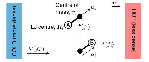 Figure 1
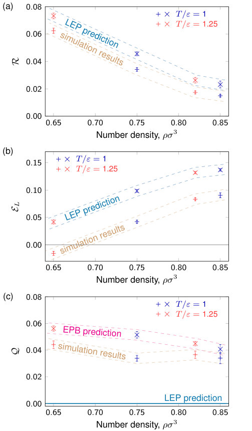 Figure 2
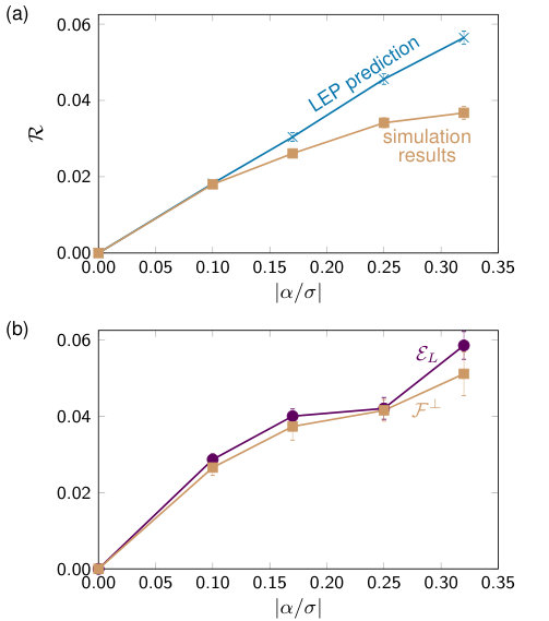 Figure 3
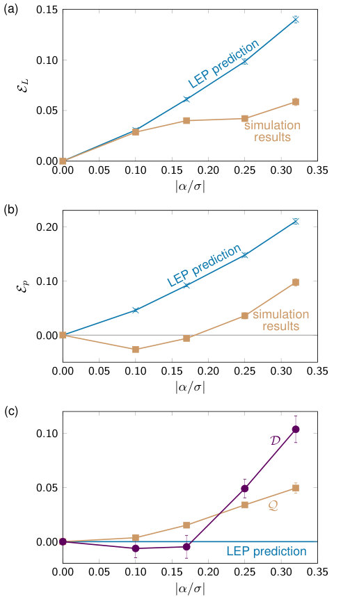 Figure 4
 Figure 5
Peer Reviews
No public reviews on file for this paper yet. If you reviewed it on a platform where reviews are public (OpenReview, ICLR, NeurIPS, ICML), you can paste yours below so the community can read it here.
Videos
No videos yet. Explain this paper in a talk, walkthrough, or lecture? Add one.
Microscopic analysis of thermo-orientation in systems of off-centre Lennard-Jones particles
Robert L. Jack
Department of Chemistry, University of Cambridge, Lensfield Road, Cambridge CB2 1EW, United Kingdom
Department of Applied Mathematics and Theoretical Physics, University of Cambridge, Wilberforce Road, Cambridge CB3 0WA, United Kingdom
Peter Wirnsberger
Department of Chemistry, University of Cambridge, Lensfield Road, Cambridge CB2 1EW, United Kingdom
Aleks Reinhardt
Department of Chemistry, University of Cambridge, Lensfield Road, Cambridge CB2 1EW, United Kingdom
Abstract
When fluids of anisotropic molecules are placed in temperature gradients, the molecules may align themselves along the gradient: this is called thermo-orientation. We discuss the theory of this effect in a fluid of particles that interact by a spherically symmetric potential, where the particles’ centres of mass do not coincide with their interaction centres. Starting from the equations of motion of the molecules, we show how a simple assumption of local equipartition of energy can be used to predict the thermo-orientation effect, recovering the result of Wirnsberger et al. [Phys. Rev. Lett. 120, 226001 (2018)]. Within this approach, we show that for particles with a single interaction centre, the thermal centre of the molecule must coincide with the interaction centre. The theory also explains the coupling between orientation and kinetic energy that is associated with this non-Boltzmann distribution. We discuss deviations from this local equipartition assumption, showing that these can occur in linear response to a temperature gradient. We also present numerical simulations showing significant deviations from the local equipartition predictions, which increase as the centre of mass of the molecule is displaced further from its interaction centre.
††thanks: current employer: DeepMind, London, United Kingdom.
I Introduction
The responses of fluids to non-equilibrium forcing can be rich and surprising. For example, temperature gradients can drive thermophoretic motion Duhr and Braun (2006); Burelbach et al. (2018); Ganti, Liu, and Frenkel (2017) as well as instabilities to convection Rosenblat and Tanaka (1971). For fluids whose molecules lack inversion symmetry, one may observe spontaneous alignment of molecules along a thermal gradient Römer et al. (2012); Daub et al. (2016); Lee (2016); Wirnsberger et al. (2018); Gardin and Ferrarini (2019); Olarte-Plata and Bresme (2019); this is known as the thermo-orientation effect. If the molecules in the fluid are polar, such a spontaneous orientation results in an emergence of electrical polarisation, or ‘thermopolarisation’, as found in computer simulations of water Bresme et al. (2008); Muscatello et al. (2011); Armstrong and Bresme (2013); Iriarte-Carretero et al. (2016); Wirnsberger et al. (2016) and other fluids Daub, Åstrand, and Bresme (2014); Lee (2016); Wirnsberger et al. (2017, 2018). Thermopolarisation and thermo-orientation effects are thought to have a common origin Römer et al. (2012); Lee (2016); Wirnsberger et al. (2018); in the following, we consider non-polar molecules without any electrostatic interactions, so our analysis is restricted to the thermo-orientation effect. However, we anticipate the principles described here can also be applied to thermopolarisation.
The analysis of such non-equilibrium effects is challenging: in contrast to equilibrium situations, methods that start from the Gibbs–Boltzmann distribution can no longer be applied, and the standard methods of equilibrium statistical physics lose much of their power. If deviations from equilibrium are small, then one may exploit ideas of non-equilibrium thermodynamics de Groot and Mazur (1984), but this is a macroscopic theory, so its predictive power for molecular properties is limited.
Alternatively, one may use methods based on kinetic theory, starting from microscopic equations of motion and adopting a mechanical approach based on the balance of forces and torques. This leads to the hierarchy of equations due to Bogolyubov, Born, Green, Kirkwood and Yvon (BBGKY) Hansen and McDonald (2006). These equations provide a detailed microscopic description of the non-equilibrium steady state, but their analysis is feasible only if the complexity of the many-particle system can be simplified in some way. In gases, one may attack these equations directly by estimating the effects of collisions on particle positions and momenta Chapman and Cowling (1990). In liquids, one more commonly works with equations of motion for hydrodynamic variables (as in the approach of Irving and Kirkwood Irving and Kirkwood (1950)), which can be closed by means of constitutive equations. Recently, methods that derive fluid properties directly from equations of motion have seen a resurgence of interest in non-equilibrium systems, particularly in active matter Takatori, Yan, and Brady (2014); Solon et al. (2015); Winkler, Wysocki, and Gompper (2015); Speck and Jack (2016); Steffenoni, Falasco, and Kroy (2017); Klymko, Mandal, and Mandadapu (2017), including methods based explicitly on force and torque balance Takatori, Yan, and Brady (2014); Steffenoni, Falasco, and Kroy (2017); Klymko, Mandal, and Mandadapu (2017). Here, we use these methods to analyse thermo-orientation.
A recent article Wirnsberger et al. (2018) presented a theory which can predict the degree of thermo-orientation based on molecular parameters and the equation of state of a (non-polar) reference fluid. The theory starts from a thermodynamic perspective and its derivation requires several assumptions about the response of individual molecules to ‘ideal’ (thermodynamic) forces. In this work, we analyse these phenomena via the equations of motion of individual particles. Our approach recovers the results of Ref. Wirnsberger et al., 2018 and also accounts for some deviations between theory and simulation seen in that work. Moreover, our results provide a deeper understanding of the nature of the non-equilibrium steady state, including formulae for a (non-Boltzmann) probability distribution of single-particle properties.
The form of the paper is as follows. Sec. II defines the model and states is governing equations. Sec. III describes the theory and the main physical insights that it provides. In Sec. IV, we present numerical results, while Sec. V contains our conclusions. Technical aspects of the theoretical calculations are included in appendices.
II Model
II.1 Equations of motion for particles
We focus on the simplest model for thermo-orientation that was considered in Ref. Wirnsberger et al., 2018. Consider a fluid of identical particles interacting by Lennard-Jones (LJ) interactions. We work in dimensions, although our results also apply for . Particle has an orientation that is encoded in a unit vector , and its LJ interaction centre is displaced by from the centre of mass. Hence, the interaction potential between particles and is , with and , where is the particle diameter and is the interaction energy. Each particle has mass and moment of inertia , which we assume to be a scalar. We also define a dimensionless ‘molecular shape parameter’ . In our numerical simulations, the moment of inertia is , corresponding to a spherical mass distribution with diameter . The temperature is measured in units such that Boltzmann’s constant .
In Fig. 1, we show a schematic of the thermo-orientation effect. The fluid is coupled to a hot and a cold reservoir. After an initial transient period that depends on initial conditions, the system converges to a steady state in which there is a temperature gradient . Let be a unit vector parallel to and let
[TABLE]
be the normalised (scalar) temperature gradient. In our simulations, is the unit vector along the axis. Following Ref. Wirnsberger et al., 2018, our theory also includes an external body force of magnitude parallel to , acting on the particles’ centres of mass. Our analysis concerns linear responses to and . We assume that there are no particle currents in the steady state of the system, as in Ref. Wirnsberger et al., 2018. In response to the temperature gradient and the external force, the system will develop a density gradient parallel to . For convenience, we define the normalised density gradient in the same manner as the temperature gradient above, namely .
Let be the (total) force exerted on particle by the other particles. The equations of motion for this particle are
[TABLE]
where is the linear momentum, is the angular momentum and . The quantity is a constant of motion: we set for all particles. Let
[TABLE]
be the particle density at position in the steady state of the system. In this formula, the angle brackets (without any subscript) indicate an average in the steady state of the system; the (Dirac) delta means that the mean number of particles in any spatial domain can be obtained by integrating over that region. For any single-particle observable , we also define the conditional average of for particles at . We denote this average by angle brackets with subscript , that is
[TABLE]
where we have used Eq. (3). A central object of interest in this work is the molecular alignment
[TABLE]
which measures the extent to which particle orientations are aligned with the temperature gradient or the applied body force.
II.2 Equations of motion for correlation functions
We consider steady-state correlation functions such as and . As an example, take , which denotes a Cartesian component of the vector (so ). We compute the time derivative of the relevant expectation value and simplify it by using the equations of motion (as in Ref. Irving and Kirkwood, 1950), giving
[TABLE]
Throughout this article, we use implicit summation over repeated Cartesian indices (in this case ). The derivative of the delta function may appear problematic, but the expectation value involves an integral over , so that all ambiguities can be avoided by integrating by parts. In addition, we have , and we note that the expectation value is taken at steady state, so the time derivative of the expectation value must vanish. Hence
[TABLE]
where indicates a derivative with respect to . Since the expectation value is a continuous function of , this derivative exists. This equation is a force-balance condition for particles at . It may be alternatively be written as
[TABLE]
which balances a body force per unit volume (left-hand side) with the divergence of the momentum flux (right-hand side).
II.3 One-particle Liouville equation
Average forces and fluxes are useful, but to obtain a more detailed analysis of the non-equilibrium steady state, we consider the probability distribution for the full state (orientation, linear momentum and angular momentum) of a particle at ,
[TABLE]
The mean force acting on a particle with this state is
[TABLE]
which depends in general on . Applying the same methodology as we did when simplifying Eq. (6), one may enforce that the time-derivative of the steady-state distribution must vanish. The result is
[TABLE]
where we emphasise that depends on , while and both depend on . This result may also be identified as the first equation of the BBGKY hierarchy. Multiplying Eq. (11) by and integrating over , and recovers Eq. (8). In fact, Eq. (11) describes the balance of all possible one-body forces and fluxes, and individual balance conditions can be obtained from it by suitable integrals. We also emphasise that this formula is valid for positions in the bulk of the system, far from any reservoirs.
III Theory of thermally induced alignment
III.1 Motivation
The central object of interest in this study is as defined in Eq. (5). Using the notation we introduced above, the key prediction of Ref. Wirnsberger et al., 2018 for this system can then be summarised as
[TABLE]
This formula is predictive because is the (imposed) temperature gradient, and can be computed from the equation of state (see below). In this equation, we wrote as shorthand notation for . We will continue to use this notation in cases where there is no ambiguity; similarly, will indicate . Eq. (12) is given here using slightly different notation from that used in Ref. Wirnsberger et al., 2018; we explain these differences in Appendix A.
We will show how Eq. (12) can be related to the equations of motion [Eq. (2)] and the Liouville equation [Eq. (11)]. The analysis is based on formulae that describe the extent to which equipartition of energy operates in this non-equilibrium steady state. Note that our analysis includes the possibility of external forces that act on the particle centres of mass, so the molecular alignment can already be finite in equilibrium states, which correspond to . We return to this point below.
III.2 Torque balance in linear response
To obtain information about the molecular alignment, it is useful to derive a torque-balance condition that is analogous to the force-balance equation [Eq. (8)]. One starts from an equation similar to Eq. (6), but replacing by . The analogue of Eq. (8) is
[TABLE]
where we used and the vector product identity . The expectation value on the right-hand side of Eq. (13) vanishes in linear response, and the additional spatial gradient means that this term contributes at third order in the temperature gradient. We therefore neglect it in the following. This leads to
[TABLE]
This equation, together with the force-balance equation [Eq. (8)], plays a central role in what follows.
III.3 Local equipartition (LEP) approach
To make progress, we must evaluate the averages involving momentum co-ordinates in Eqs (8) and (14). At equilibrium (), this can be done by equipartition of energy. In the linear response regime (small ), it is still consistent to use the equilibrium equipartition formula in Eq. (8). (Corrections to equilibrium equipartition enter Eq. (8) only at third order.) Taking the scalar product with the unit vector yields
[TABLE]
We identify the ideal pressure as and the gradient of the excess pressure as . The left-hand side of Eq. (15) therefore corresponds to the external force per unit volume and the right-hand side corresponds to the gradient of the (total) pressure: this is mechanical equilibrium, . If the equation of state of the fluid is known, this means that the density gradient can be computed, which enables determination of .
For systems out of equilibrium, we will show that it is not consistent to use equilibrium equipartition formulae to average the angular momenta in Eq. (14). In fact, consistency with Ref. Wirnsberger et al., 2018 requires that we take
[TABLE]
where we recall that is the position of the LJ centre of the molecule. That is, a form of equipartition still holds, but the temperature is to be evaluated at the position of the LJ centre, which we also identify as the ‘thermal centre’ of the molecule. At equilibrium, and one recovers the equilibrium result: the factor of enters because , so the angular momentum has independent components. A first-order Taylor expansion of the temperature in Eq. (16) about the centre of mass gives
[TABLE]
The second term on the right-hand side is proportional to the distance between the molecular centre of mass and its thermal centre. The pre-factor of this term could be altered by replacing in Eq. (16) by some other position within the molecule. However, we will see later that Eq. (16) is not arbitrary: it is constrained by the form of the Liouville equation [Eq. (11)].
We assume additionally that the molecular force is uncorrelated with its orientation,
[TABLE]
where we used by independence and , which is valid in linear response because the orientation is a unit vector that is distributed isotropically at zeroth order. At equilibrium (), Eq. (18) does hold; the LEP assumption is that it remains true away from equilibrium. Combining Eqs (14), (17) and (18) yields Eq. (12).
Note that if the temperature is constant throughout the system, then the assumptions of Eqs (16) and (18) are exact: they can be derived from the Boltzmann distribution. In this case, Eq. (12) is exact and together with Eq. (15) yields . This result, which was verified numerically in the ‘ runs’ of Ref. Wirnsberger et al., 2018, gives an exact prediction of particle orientation in equilibrium states with applied external forces, at the level of linear response.
III.4 Physical interpretation of LEP
We have derived Eq. (12) from the molecular equations of motion [Eq. (2)] using the assumptions of Eqs (16) and (18). This approach gives a microscopic theoretical foundation for the arguments of Ref. Wirnsberger et al., 2018. We will discuss these assumptions in more detail below and compare them to numerical simulations. However, before doing so, we summarise the overall physical picture illustrated in Fig. 1.
For thermo-orientation in the absence of an external body force, the ideal pressure gradient in Eq. (15) is non-zero, and it must be balanced by the interparticle force . The ideal pressure gradient is the divergence of the momentum flux: particles move more slowly in cold regions, so the time spent there tends to be longer. The interparticle force balances out this tendency. This force acts on the LJ centre and thus exerts a torque on the molecule (recall Fig. 1). Hence the force appears in the torque-balance equation [Eq. (12)].
However, molecular alignment also displaces particles’ thermal centres and changes their kinetic energies. This favours configurations where the thermal centres are closer to the cold bath, since the reduced angular velocity means that particles stay longer in these configurations. This effect generates the temperature-gradient term in Eq. (12). In the example considered here, the two contributions to the right-hand side of Eq. (12) have opposite signs, with the temperature-gradient term being larger in magnitude. This mechanical derivation and interpretation of Eq. (12) are the first key insight of this paper.
It is useful to note at this point that this LEP construction is straightforwardly extended to arbitrary shaped molecules, along the lines discussed in Ref. Gardin and Ferrarini, 2019. The arguments of the following Section III.5 can also be extended, but in that case the position of the thermal centre cannot be deduced from the equations of motion, in contrast to the off-centre LJ particles considered here.
III.5 LEP distribution
The assumptions of Eqs (16) and (18) may seem arbitrary at this stage. We now show that these results can be justified in terms of a one-body probability distribution that solves the Liouville equation [Eq. (11)]. That is, while alternative assumptions might appear plausible, they would not typically be consistent with Eq. (11).
We will introduce several ansätze for , of the form
[TABLE]
where is a normalisation constant, is a smooth function and enforces that is a unit vector and is perpendicular to . The simplest ansatz for is that only the kinetic energy is correlated with the position: this motivates the name ‘local equipartition’. It means that
[TABLE]
where is a parameter related to the molecular alignment, is the vector from the centre of mass to the thermal centre (we are treating as an adjustable parameter), and
[TABLE]
is the kinetic energy. (Recall , so .) In Eq. (19), is the value of the temperature at the thermal centre. It is shown in Appendix B.2 that the ansatz (19) is consistent with Eq. (11) only if the mean force on the particle is
[TABLE]
where is the mean kinetic energy and is another parameter. In addition, Eq. (11) imposes
[TABLE]
which is equivalent to Eq. (15) since , and
[TABLE]
The last result for means that the thermal centre in Eq. (19) must indeed coincide with the LJ centre, as we claimed above.
Evaluating averages with respect to , one finds in linear response that
[TABLE]
which together with Eq. (23) imply Eq. (12). The other LEP assumptions [Eqs (16) and (18)] can also be derived as averages with respect to . Also, similarly to Eq. (17), we have
[TABLE]
The conclusion of this analysis is that the LEP distribution and its associated force describe a consistent physical picture, at the one-body level, of the behaviour of molecules in this system. If the equation of state of the fluid is given, then the distribution has no adjustable parameters. This picture is fully consistent with Ref. Wirnsberger et al., 2018 and has the same implications. However, the LEP distribution also makes predictions for other correlation functions, beyond those considered so far.
In fact, our numerical results (Sec. IV) show that the LEP distribution does not provide a full description of the linear response of this fluid. To this end, we discuss some corrections to this distribution.
An important feature is that the LEP distribution is time-reversal symmetric (i.e. it is invariant under reversal of all momenta), so it cannot describe dissipative effects such as heat currents, which will be present if . Dissipative effects lead to non-zero values of correlation functions that are odd under time reversal, such as . Eq. (19) can be modified in order to incorporate such correlations, but within linear response, these modifications have no effect on non-dissipative (time-reversal-symmetric) quantities such as the molecular alignment. We therefore neglect dissipative terms in the following. However, there are also corrections to LEP that do affect the molecular alignment, which we discuss in Sec. III.6.
III.6 Equipartition breaking (EPB)
We consider alternative solutions to Eq. (11), which we write in terms of a function as
[TABLE]
Here EPB indicates an ‘equipartition-breaking’ solution (and note that indicates a change in , the does not indicate any kind of delta function). Similarly
[TABLE]
The factors of in these equations highlight that corrections to LEP are assumed to be linear in the deviation from equilibrium, and are odd in . Expansions similar to Eq. (25) have been considered before in kinetic theory Chapman and Cowling (1990) and also (for example) when analysing systems where energy is slowly injected into a homogeneous system, during a chemical reactionde Groot and Mazur (1984); Ross and Mazur (1961). In general, one expects that the Maxwell-Boltzmann distribution for can be perturbed by the thermal gradient, and also that the internal degrees of freedom of the molecule (orientation and angular momentum ) can become correlated with , and with each other. In the situation considered here, we emphasize that must be odd in : the terms that appear at first order in our expansion change sign if the temperature gradient is reversed. This symmetry greatly simplifies the analysis by restricting the terms that can appear in our ansatze for and . One possible correlation, consistent with this symmetry, is that particles whose orientations are aligned with the temperature gradient () have slightly higher kinetic energies, compared with particles that are anti-aligned (). See Eqs. (29,30) below.
We have found a three-parameter family of EPB solutions, which depend on (dimensionless) free parameters , and . We note that this solution is specific to this system, in which all intermolecular forces act via a single ‘force centre’. This means that the only difference between the forces and in Eq. (2) is the external force. This places strong constraints on the possible solutions to Eq. (11), and enables this analysis. The formulae that describe the EPB solutions are somewhat unwieldy: we first state them and then discuss their physical consequences.
The EPB distribution has
[TABLE]
and the associated mean force is
[TABLE]
where we recall . The consistency of these formulae with Eq. (11) is demonstrated in Appendix B.3.
The parameters , and are not predicted within this theory, so this general form for does not allow predictions from first principles, contrary to LEP. However, the EPB theory does enforce relations between correlation functions that come from the equations of motion, such as Eq. (14). Hence, if , and are obtained by measuring certain correlation functions, then the values of other correlation functions can be predicted. If all these parameters are zero, then we recover LEP.
For the cases considered below, , and are all positive and of similar magnitudes. The physical implications of these parameters become apparent when we compute correlation functions (see also Appendix C). For example, instead of Eq. (17), we find
[TABLE]
The LEP case corresponds to . We see that positive corresponds to a weaker correlation between a particle’s angular momentum and its orientation compared with LEP. Similarly
[TABLE]
Based on these equations, one possible physical interpretation is that the thermal centre of the molecule is displaced away from the LJ centre towards the centre of mass. However, we argue that this is not appropriate: a key feature of EPB is that one cannot use a single thermal centre to account for the statistics of both linear and angular momentum.
As well as modified equipartition formulae, EPB also predicts correlations of molecular properties with the force. For example, Eq. (18) becomes
[TABLE]
The LEP case is , in which case the left-hand side is zero, consistent with Eq. (18). The EPB distribution predicts that the force is correlated with the molecular orientation. In particular, for , it predicts that the intermolecular force tends to be larger when the molecules are either parallel or antiparallel to the temperature gradient. This effect tends to reduce the torque on the particles.
Combining the torque-balance condition [Eq. (14)] with Eqs (29) and (31) leads to a modified prediction for the molecular alignment,
[TABLE]
which generalises Eq. (12). Note that if for some reason we have , then Eq. (12) may still hold to high accuracy, even if the LEP assumptions [Eqs (16) and (18)] have significant violations.
We have seen that and are related to deviations from equipartition, and also have implications for correlations between force and orientation. The third parameter is related to coupling between linear and angular momentum. For example, one has
[TABLE]
Another quantity related to equipartition is
[TABLE]
One notes that among the five correlation functions [Eqs (29)–(31), (33) and (34)], there are only three independent parameters, , and . These constraints on correlation functions arise from the form of the Liouville equation [Eq. (11)]. For example, in Appendix C, Eq. (79) is derived directly from the equations of motion (in linear response). It can be rearranged to give
[TABLE]
This result must hold for any solution of the Liouville equation, which of course includes the EPB solution. Note however that Eq. (31) cannot to our knowledge be derived directly from the equations of motion: it seems to be a specific property of the EPB solution.
III.7 Physical interpretation of EPB
Physically, we interpret and in terms of the correlations between orientation and the kinetic energy of a particle, from Eqs (29) and (30). If and , the kinetic energy of a particle is less strongly correlated with its orientation than is predicted by LEP. Similar effects could also be achieved by assuming that the thermal centre of the molecule is somewhere between the LJ centre and the molecular centre of mass, instead of at the LJ centre, as in LEP. However, the form of Eq. (27) and the fact that the correlation function in Eq. (34) is non-zero within EPB both show that the state described by Eq. (27) cannot be accounted for by assuming the existence of a single thermal centre.
In numerical simulation (see Sec. IV), the parameters and can be estimated by considering correlations of orientation and velocity. This leads to non-trivial predictions for the correlations between the interparticle force and the velocity, via Eq. (28). In particular, one sees from Eq. (31) that the correlations between velocities and orientations can only be sustained if there are also correlations of the interparticle force with the orientation.
The parameter is different in that it does not appear in the expression for the mean force [Eq. (28)]. In this sense, it encodes correlations among particle velocities that do not require any (mean) force to sustain them. Our numerical results (see below) are consistent with , and all being of comparable magnitudes, with typical values in the range –.
IV Numerical results
IV.1 Calculation method
We obtained numerical results using a modified version of the LAMMPS simulation package Plimpton (1995) (v. 11Aug17), with the same methods as Ref. Wirnsberger et al., 2018. The system is periodic, with box dimensions , and comprises 5832 off-centre LJ particles. The box length is chosen to produce the desired overall number density, and in our simulations is of the order of . The LJ interaction is truncated at and the time step was . There is a temperature gradient along the direction, which is achieved by imposing different temperatures in two equally spaced thermal baths, each of width . The temperature in these regions is controlled using local Gaussian thermostats that act on the non-translational kinetic energy of the reservoir and leave the centre of mass motion unaffected, as in Ref. Wirnsberger et al., 2018. After equilibration at an appropriate state point Wirnsberger et al. (2018), the Gaussian thermostats were activated and the system was simulated for a time , in order to establish the non-equilibrium steady state. This was followed by production runs of . (These long simulations are necessary because the magnitude of the thermo-orientation effect is small, so significant averaging is required in order to obtain small statistical uncertainties.)
We partitioned the system into 20 segments along the direction and computed single-particle observables of interest independently within each segment. The results shown here are averaged over the segments, but excluding regions that are overlapping with or close to the thermal baths. The dependence of the results on is very weak in all cases, consistent with the small imposed temperature gradient. Error bars are computed by assuming that measurements within each segment are independent and calculating the standard error. Similar error estimates could also be obtained by analysing how the results fluctuate as a function of time. In addition to the results shown here, we also carried out some simulations with a smaller time step . These simulations reached shorter times so there is less data to average over, hence numerical uncertainties are larger. However, we did not find any evidence for significant dependence of our results on the timestep.
IV.2 Dependence of orientation on
This section shows results for several state points, which are labelled by (average) temperatures and . The heat baths are maintained at and . The local temperature in simulations is determined as : this varies linearly with in the region outside the baths. The temperature gradient is measured using data for the local temperature, in the region outside of the baths. This leads to values of between and .
Since these gradients are small, the responses are also small, and we therefore normalise all responses by the size of the gradient itself. To this end, we define dimensionless observables, which all have the property that they are independent of within the linear response regime. The response of the orientation to the gradient is
[TABLE]
The normalised interparticle force is
[TABLE]
With this choice, and since is a unit vector in the direction, the LEP prediction [Eq. (12)] for the alignment, which is also the prediction of Ref. Wirnsberger et al., 2018, is
[TABLE]
Note that throughout our numerical work. In this section, we take , as in Ref. Wirnsberger et al., 2018. The LEP prediction of Eq. (38) is tested in Fig. 2(a), for several values of . There is good, but not perfect, agreement between the prediction and the numerical results. The deviations are comparable with those found in the NEMD (non-equilibrium molecular dynamics) simulations of Ref. Wirnsberger et al., 2018.
It is also notable that the response decreases with density. This is expected because Eqs (12) and (15) with together imply , so the response is proportional to the induced density gradient . As the fluid gets denser, the compressibility is reduced, so decreases, and so does the thermo-orientation effect.
To test the LEP theory in more detail, we define two quantities that measure the correlation between orientation and kinetic energy,
[TABLE]
The minus signs in these definitions are somewhat arbitrary: they are included so that and are positive in our numerical calculations, which means that the orientation is anti-correlated with the kinetic energy. We also define
[TABLE]
which measures the correlation between the interparticle force and the orientation. The LEP predictions [Eqs (17) and (18)] are that
[TABLE]
These two predictions are tested in Fig. 2(b, c). One sees significant violations of these predictions, which are larger than the deviations from Eq. (38) that are apparent in Fig. 2(a). In Sec. III.3, assumptions equivalent to Eqs (42) and (43) were used to derive the result given by Eq. (12), which is equivalent to Eq. (38). The results of Fig. 2 show that the final result holds more accurately than the assumptions that were used to derive it. Clearly, some cancellation of errors is at work.
To investigate this, we consider the EPB theory, which has adjustable parameters and . To estimate them, we use the EPB predictions of Eqs (29) and (30) to write
[TABLE]
Hence may be estimated from the data. (If LEP holds, then .) Once and are fixed, then Eq. (31) is a non-trivial prediction of EPB theory. It implies that
[TABLE]
This prediction is tested in Fig. 2(c). We note that in contrast to LEP, which predicts , the EPB prediction gives the correct (positive) sign for . However, the numerical results still deviate from the EPB prediction. Recalling Eq. (41), we observe from Fig. 2(c) that the force tends to be either parallel or anti-parallel to (recall ). Hence, the mean torque on the molecule is reduced, compared to the LEP theory. This situation is similar for all four state points considered. We now fix a single state point and study its behaviour in more detail, focussing on the dependence of thermo-orientation on .
IV.3 Dependence of orientation on
We focus on and , and we consider how the results depend on . For , there is no thermally induced alignment, so it is natural to expect responses proportional to when . However, we emphasise that there is no assumption of small within our theory: we consider linear response to the thermal gradient , but our theory can in principle capture non-linear dependence on .
Fig. 3(a) shows the response as a function of , and the comparison with the LEP prediction of Eq. (12). [The points for were already shown in Fig. 2(a).] The LEP prediction is almost linear in , because the mean force in Eq. (12) depends very weakly on . The numerical results show a saturation in the thermo-orientation as is increased, which is not captured by Eq. (12). We have checked that this result is not associated with a breakdown of linear response in : for , we reduced the temperature gradient by a factor of two, which led to very small change in (the difference was less than and within the range of error bars). The conclusion is that LEP is violated at the level of linear response to the temperature gradient. This is consistent with the EPB theory.
We now consider the torque-balance equation [Eq. (14)]. We define a normalised torque as the projection of the interparticle force perpendicular to the orientation,
[TABLE]
so that Eq. (14) is equivalent to
[TABLE]
From Fig. 3(b), we see that the equation is obeyed, up to numerical and statistical uncertainties. It was derived directly from the equations of motion, up to our neglect of the right-hand side of Eq. (13), which we have separately verified to be very small [at least one order of magnitude smaller than the quantities plotted in Fig. 3(b)]. Since Eq. (14) does not rely on LEP nor on linear response, any deviations from this prediction would have to be attributed to errors associated with our numerical integration of the equations of motion.
We now test in detail the predictions of LEP, which include Eqs (42) and (43), as well as Eq. (24), which is equivalent to
[TABLE]
We also define
[TABLE]
and note that LEP predicts
[TABLE]
The predictions of Eqs (42), (43), (48) and (50) are all tested in Fig. 4. It is interesting to note that while the LEP prediction in Fig. 3(a) is accurate for and gives a reasonable estimate of the orientation effect at , the other LEP predictions shown in Fig. 4 are much less accurate in this regime. This is a similar cancellation of errors to that observed in Fig. 2: that is, LEP gives reasonable predictions of , but less accurate predictions of other quantities.
The EPB theory provides a partial explanation of this behaviour. The theory predicts Eq. (32), which is equivalent to
[TABLE]
We can compare this expression with Eq. (38): the difference is in the term . Fig. 5(a) shows estimates of and using Eq. (44). Both are positive and significantly different from zero, consistent with the deviations from LEP seen in Fig. 4(a, b). Note also that our results are consistent with and as , so that LEP appears to hold for small .
The key point is that and are numerically similar, which means that the EPB contributions to Eq. (51) are small, even though the individual values of and indicate significant violations of LEP. Results are shown in Fig. 5(b), compared with the EPB prediction [Eq. (45)]. For , our results are consistent with EPB theory: we have and the LEP prediction for is still accurate, even if other LEP predictions fail. For , the EPB theory still gives better qualitative predictions than LEP, but we also observe significant deviations, consistent with Fig. 2(c). While the LEP theory predicts , the EPB theory gives the right sign for and is accurate for small , but there are deviations for larger values of .
Finally, we note from Eq. (33) that
[TABLE]
For , where the EPB theory is reasonably accurate, one may then use the results of Fig. 5 to estimate , which is positive and similar in magnitude to both and . Within the framework presented here, we have no explanation of this apparent coincidence. The smallness of is the source of the cancellation of errors in the LEP prediction of , so it would be useful to have an explanation of this effect. It is notable that for , the first term in Eq. (27) is proportional to the squared velocity of the LJ centre of the molecule, but a more detailed analysis of the structure of is beyond the scope of this work.
V Conclusion
We have shown how a theory of thermo-orientation can be derived directly from the equations of molecular dynamics. The central idea is that the form of the one-particle Liouville equation [Eq. (11)] places constraints on steady-state correlation functions of the non-equilibrium fluid. The mean force in that equation depends on the orientation and velocity of the particle, and this dependence is not known. However, we have presented two possible types of solution for Eq. (11), which are associated with specific forms for . One of these solutions corresponds to a local equipartition assumption (LEP) and the other to a non-trivial state where local equipartition is broken (EPB). The LEP assumption recovers the prediction of Ref. Wirnsberger et al., 2018 for thermo-orientation in this system. The EPB assumption shows how deviations from LEP can appear even at linear response in the temperature gradient.
We have also presented numerical results. For molecules where the centre of mass is close to the interaction centre (small ), the LEP theory is very accurate. For , there are significant deviations from LEP. The EPB theory can capture some of these deviations by appropriate choices of fitting parameters. This theory also makes a non-trivial prediction [Eq. (45), equivalent to Eq. (31)] which improves on the LEP prediction but is still not fully consistent with the numerical results. This indicates that the EPB theory is not a full description of the non-equilibrium steady state, even in the linear-response regime.
The detailed EPB theory is restricted to the system considered here, because specifying the mean force in the Liouville equation means that the mean torque on the molecule is also fully determined. However, the structure of the LEP solution is quite general, and can be analysed in other cases too. For future directions, one might include electrostatic polarisation in the theory Wirnsberger et al. (2018) as well as investigating in more detail the accuracy of LEP for particles with different shapes Gardin and Ferrarini (2019).
Another possible direction would be to connect with classical kinetic theory calculations that start from the Boltzmann equation Chapman and Cowling (1990); Ross and Mazur (1961). This might lead to additional constraints on the terms appearing in the expansion (26) for , as well as helping to relate these terms to microscopic physical processes. The link to kinetic theory also suggests that one might investigate thermo-orientation in fluids that are more dilute, instead of dense liquids. For example, an expansion in powers of the density might offer a systematic characterisation of the possible orientational responses to temperature gradients, and their expected magnitudes.
Acknowledgements.
We thank Daan Frenkel, Christoph Dellago, Kranthi Mandadapu, and Ronojoy Adhikari for helpful discussions. P.W. is grateful for a Microsoft Azure Research Sponsorship. The results presented here were achieved in part using the Vienna Scientific Cluster. The data generated during this study are available at https://doi.org/10.17863/CAM.37306.
Appendix A Connection to previous studies
In Eq. (5) of Ref. Wirnsberger et al., 2018, the alignment of non-polar molecules is computed via
[TABLE]
where is a force that acts at the LJ centre of the molecule, and we have used explicitly. The physical picture of Ref. Wirnsberger et al., 2018 is that the various terms in our Eq. (15) are all identified as forces (acting along the direction, which is the direction of ). In particular, and are referred to as ‘ideal forces’. Moreover, the ideal force is identified as acting at the LJ centre, so it contributes to in Eq. (53), while the other ideal force is identified as acting at the centre of mass.
In more detail, the correspondence with Ref. Wirnsberger et al., 2018 is
[TABLE]
where the forces of Ref. Wirnsberger et al., 2018 are on the left and the corresponding quantities in this work are on the right. One sees that Eq. (15) of this work corresponds to force balance , as in Ref. Wirnsberger et al., 2018. Combining Eq. (53) with Eq. (54) and noting also recovers Eq. (12).
We reiterate that the assignment of the ideal forces and to and in Eq. (54) was justified in Ref. Wirnsberger et al., 2018 on phenomenological grounds. A key result from this work is that the LEP distribution provides a microscopic basis for this choice.
Note also that all results in this work are for thermo-orientation in the absence of any external force . These were called ‘NEMD runs’ in Ref. Wirnsberger et al., 2018, which also considered ‘ runs’, in which an external force was added in order that there was no density gradient , and ‘ runs’, where there was an external force and a density gradient but no temperature gradient.
The theory presented here can be applied in all cases. However, for runs, the system is at equilibrium, and LEP predictions are exact (see Sec. III.3). We have analysed runs, and have found that the absolute differences between LEP and EPB theory are very similar to NEMD runs (i.e. those with no external force). However, the total thermo-orientation effect is much larger if the external force is applied, so the deviations between LEP and EPB are less apparent in the runs. The NEMD case is the one of primary interest, and it is also the most challenging for the theory, hence we focus on that case.
Appendix B Solutions to the one-particle Liouville equation
This appendix shows that the LEP and EPB distributions are consistent with the Liouville equation Eq. (11). Define an equilibrium-like distribution
[TABLE]
where the kinetic energy is given by Eq. (20). We seek solutions to Eq. (11) of the form for some function . As usual, we work in the linear response regime; at zeroth order then . Dividing Eq. (11) by and defining yields
[TABLE]
where is the mean kinetic energy. We note that , , ,, and are all small in the linear response regime where we work. Keeping terms at first order and rearranging the order of some terms, we obtain
[TABLE]
where we have also rearranged some terms using vector product identifies, particularly .
We note that the derivatives with respect to and in Eq. (56) treat the orientation and angular momenta as vectors with three components, but we are restricting to cases where is a unit vector and . One may also verify this analysis with being represented explicitly as a point on the unit sphere, so that the vector is tangential to the sphere. For the angular momentum, a consistent analysis requires that is independent of .
B.1 Boltzmann solution (for )
We first consider the case where there is no temperature gradient, but an external force is applied. The system is at equilibrium but the force does induce an alignment of the particles, as in the ‘ runs’ of Ref. Wirnsberger et al., 2018. It is useful to write
[TABLE]
and
[TABLE]
Here are constants, independent of , and . One may interpret as a first-order Taylor expansion of an orientational distribution , where is a free energy gain (normalised by the temperature) for alignment of with . Assuming (57,58) and setting , consistency with Eq. (56) requires
[TABLE]
The form of also implies , so this is also consistent with Eqs (12) and (15).
B.2 LEP solution
In the Boltzmann case, Eq. (56) is linear in momenta. In this case, is independent of momenta. However, if , then Eq. (56) contains terms cubic in momenta, due to the presence of the kinetic energy . In the LEP solution, one chooses so that the term proportional to in Eq. (56) is cancelled by the term proportional to . This requires
[TABLE]
as in Eq. (21). With this choice, the term in Eq. (56) proportional to generates an additional non-linear term that is cancelled by the term proportional to , which requires
[TABLE]
This choice, together with Eq. (21), ensures the cancellation of all terms in Eq. (56) that are non-linear in momenta. Next, one must choose and such that the linear terms cancel and Eq. (56) is satisfied. This requires that Eq. (22) holds, and that is consistent with Eq. (23). Finally, we note that Eq. (59) is consistent with Eq. (19) only if . Hence, at leading order, Eqs (19), (21), (22) and (23) are together consistent with Eq. (56) and therefore with Eq. (11), as required.
B.3 EPB solution
We now turn to the EPB distribution. Recall that the angular velocity is . From Eqs (25) and (26), one has and . Since and together already solve Eq. (56), that equation may be rewritten as
[TABLE]
We write and similarly (note ). The linearity of Eq. (60) means that if each pair (such as , ) solves Eq. (60) separately, then their sum is also a solution.
B.3.1 term
We first consider
[TABLE]
and
[TABLE]
In Eq. (60), we recall that derivatives with respect to are taken at fixed . Hence, for any fixed vector , one has
[TABLE]
Making use of this formula,
[TABLE]
Note also that
[TABLE]
Combining all these formulae and recalling , one may verify that Eq. (60) holds.
We observe that the functional forms of and are constrained by the fact the second line of Eq. (60) contains terms that are non-linear in momenta, which must all cancel. In particular, this enforces that the non-linear terms in must be proportional to , which is the same factor multiplying in Eq. (60), and may be identified as the velocity of the LJ centre of the molecule.
B.3.2 term
The analysis of this case is similar to the previous one, except that the nonlinearity in includes terms quadratic in , instead of terms quadratic in . In particular
[TABLE]
where one again notices the same factor of . Hence
[TABLE]
Also,
[TABLE]
from which one has
[TABLE]
In order to evaluate the contribution in Eq. (60), it is important that does not depend on the constant of motion . One uses to write
[TABLE]
The derivative of this expression can be evaluated as
[TABLE]
Combining Eqs (64)–(67), one may again verify Eq. (60).
B.3.3 term
The parameter does not appear in . Instead one notes that
[TABLE]
for which and so Eq. (60) holds trivially.
Appendix C Correlation functions for the LEP and EPB distributions
This Appendix shows how to compute expectation values with respect to the LEP and EPB distributions. To first order one has
[TABLE]
where was defined in Eq. (55), while comes from Eq. (59) and from Eq. (27). Hence (for any ) the EPB average is
[TABLE]
where indicates an average with respect to . Hence, all correlation functions can be reduced to averages with respect to this Gaussian distribution. We summarise some general results before computing some specific correlations. The momentum is independent of all other variables, and
[TABLE]
For the orientation one has
[TABLE]
The orientation and angular momentum are not completely independent (because ). One has
[TABLE]
Since and are independent, one also has
[TABLE]
C.1 Average orientation and force
Using the results above, one may now evaluate correlation functions. For example, the average orientation for the LEP distribution is
[TABLE]
To obtain the second line, we used the fact that is even in , as well as Eq. (59). To get to the third line, we note that is independent of the orientation. To obtain the equivalent result for the full EPB distribution requires computation of the correction . Performing the Gaussian integrals yields
[TABLE]
Similarly one sees that (to leading order)
[TABLE]
(The average of the EPB force is zero.) Using this formula with Eq. (73) and Eq. (23) yields Eq. (32).
C.2 Equipartition formulae
Having explained the general method, we sketch the computations of other correlation functions. To derive Eq. (29), which quantifies deviations from equipartition, one first considers the LEP case,
[TABLE]
Using Eq. (72) and rearranging, one has
[TABLE]
consistent with Eq. (17). The EPB correction to this quantity may be written as
[TABLE]
The only non-zero contribution to this average comes from terms proportional to . The relevant term in is , where we used the definition of . Noting that the other terms in all have vanishing contributions to the average, Eq. (75) can be reduced to
[TABLE]
This evaluates to Adding this correction to the LEP result [Eq. (74)] yields Eq. (29).
The other equipartition formula, Eq. (30), can be derived similarly. The only term in that contributes to the EPB correction is , which appears in .
C.3 Other correlation functions
To derive Eq. (31), note that and recall . Hence
[TABLE]
consistent with Eq. (31).
To derive Eq. (33), one writes
[TABLE]
There are several relevant contributions to , all of which are linear in (otherwise the correlation function vanishes). The contribution from is proportional to , which is given in Eq. (71). The contribution from is proportional to and also proportional to
[TABLE]
which evaluates to . To show this, one may first average over the momentum , which is independent of and , and then use vector product identities.
Following the same methodology, one may also show that
[TABLE]
The second equation does not include or because
[TABLE]
which may be checked by performing the average over and then using . Writing , one also sees that
[TABLE]
Hence, taking the difference of the two lines of Eq. (76) provides an alternative derivation of Eq. (33).
Finally, we note that writing Eq. (6) with replaced (on the left-hand side) by and using the equations of motion [Eq. (2)] yields
[TABLE]
where we dropped a term that vanishes in linear response. Rearranging and using Eq. (77), we have
[TABLE]
Since Eqs (78) and (79) follow directly from the equations of motion, both LEP and EPB ansätze must be consistent with them. Note that Eq. (78) relates the sum of the two correlation functions in Eq. (76) to the force-orientation correlation in Eq. (31) – it is easily checked that the EPB ansatz is consistent with this constraint.
The reference list from the paper itself. Each links out to its DOI / PubMed record.
- 1Duhr and Braun (2006) S. Duhr and D. Braun, “Why molecules move along a temperature gradient,” Proc. Natl. Acad. Sci. U. S. A. 103 , 19678 (2006) . · doi ↗
- 2Burelbach et al. (2018) J. Burelbach, D. Frenkel, I. Pagonabarraga, and E. Eiser, “A unified description of colloidal thermophoresis,” The European Physical Journal E 41 , 7 (2018).
- 3Ganti, Liu, and Frenkel (2017) R. Ganti, Y. Liu, and D. Frenkel, “Molecular simulation of thermo-osmotic slip,” Phys. Rev. Lett. 119 , 038002 (2017) . · doi ↗
- 4Rosenblat and Tanaka (1971) S. Rosenblat and G. A. Tanaka, “Modulation of thermal convection instability,” Phys. Fluids 14 , 1319 (1971) . · doi ↗
- 5Römer et al. (2012) F. Römer, F. Bresme, J. Muscatello, D. Bedeaux, and J. M. Rubí, “Thermomolecular orientation of nonpolar fluids,” Phys. Rev. Lett. 108 , 105901 (2012) . · doi ↗
- 6Daub et al. (2016) C. D. Daub, J. Tafjord, S. Kjelstrup, D. Bedeaux, and F. Bresme, “Molecular alignment in molecular fluids induced by coupling between density and thermal gradients,” Phys. Chem. Chem. Phys. 18 , 12213 (2016) . · doi ↗
- 7Lee (2016) A. A. Lee, “Microscopic mechanism of thermomolecular orientation and polarization,” Soft Matter 12 , 8661 (2016) . · doi ↗
- 8Wirnsberger et al. (2018) P. Wirnsberger, C. Dellago, D. Frenkel, and A. Reinhardt, “Theoretical prediction of thermal polarization,” Phys. Rev. Lett. 120 , 226001 (2018) . · doi ↗