Convergence of the Non-Uniform Physarum Dynamics
Andreas Karrenbauer, Pavel Kolev, Kurt Mehlhorn

TL;DR
This paper proves convergence of a generalized Physarum dynamics to the optimal solution of a weighted basis pursuit problem, extending previous results from uniform cases to more general, non-uniform and functional dynamics.
Contribution
It establishes convergence for non-uniform Physarum dynamics with general reactivity functions, broadening the understanding beyond uniform and specific shortest path cases.
Findings
Convergence shown for non-uniform Physarum dynamics under general conditions.
Extended convergence results to dynamics with multiplicative factors involving functions g_e.
Demonstrated convergence for a broader class of problems beyond shortest path.
Abstract
Let , , and . We show under fairly general conditions that the non-uniform Physarum dynamics \[ \dot{x}_e = a_e(x,t) \left(|q_e| - x_e\right) \] converges to the optimum solution of the weighted basis pursuit problem minimize subject to and . Here, and are -vectors of real variables, minimizes the energy subject to the constraints and , and is the reactivity of edge to the difference at time and in state . Previously convergence was only shown for the uniform case for all , , and . We also show convergence for the dynamics \[ \dot{x}_e = x_e \cdot \left( g_e \left(\frac{|q_e|}{x_e}\right) - 1\right),\] where is an…
Click any figure to enlarge with its caption.
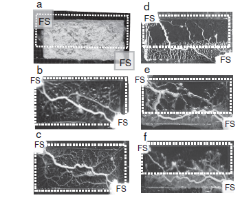 Figure 2
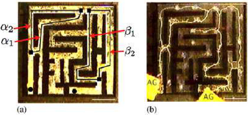 Figure 2
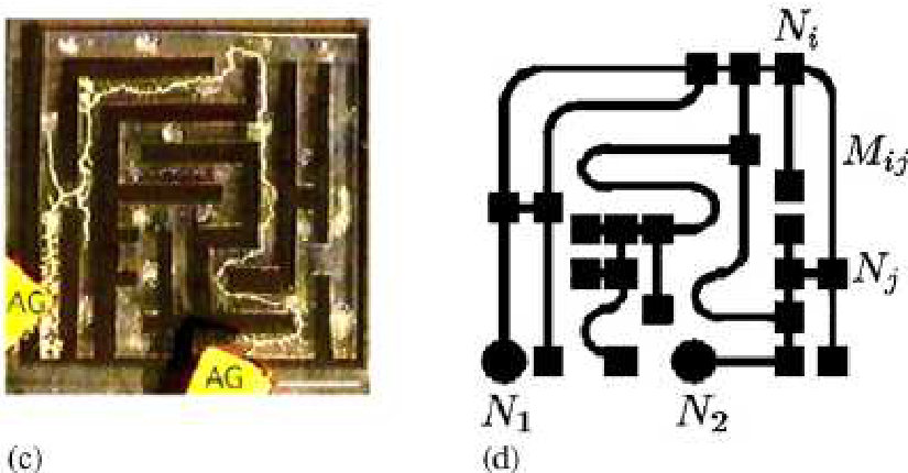 Figure 3
Peer Reviews
No public reviews on file for this paper yet. If you reviewed it on a platform where reviews are public (OpenReview, ICLR, NeurIPS, ICML), you can paste yours below so the community can read it here.
Videos
No videos yet. Explain this paper in a talk, walkthrough, or lecture? Add one.
Convergence of the Non-Uniform Physarum Dynamics
Andreas Karrenbauer Max Planck Institute for Informatics, Saarland Informatics Campus.
Pavel Kolev∗
Kurt Mehlhorn∗
Abstract
The Physarum computing model is an analog computing model motivated by the network dynamics of the slime mold Physarum Polycephalum. In previous works, it was shown that it can solve a class of linear programs. We extend these results to a more general dynamics motivated by situations where the slime mold operates in a non-uniform environment.
Let , , and . We show under fairly general conditions that the non-uniform Physarum dynamics
[TABLE]
converges to the optimum solution of the weighted basis pursuit problem minimize subject to and . Here, and are -dimensional vectors of real variables, minimizes the energy subject to the constraints and , and is the reactivity of edge to the difference at time and in state . Previously convergence was only shown for the uniform case for all , , and .
We also show convergence for the dynamics
[TABLE]
where each is an increasing differentiable function with (satisfying some mild conditions). Previously, convergence was only shown for the special case of the shortest path problem on a graph consisting of two nodes connected by parallel edges.
1 Introduction
The Physarum computing model is an analog computing model motivated by the network dynamics of the slime mold Physarum polycephalum. In wet-lab experiments, it was observed that the slime mold is apparently able to solve shortest path problems [NYT00]. A mathematical model for the dynamic behavior of the slime was proposed in [TKN07]. It models the slime network as an electrical network with time-varying resistors that react to the amount of electrical current flowing through them. A more general model for the dynamics was introduced in [NIU*+*07] to deal with situations in which the slime has to operate in a non-uniform environment. This more general dynamics is the subject of this paper. In Section 2, we give more details on the biological background and also survey the theoretical work on the Physarum dynamics.
The weighted basis pursuit problem asks to find the minimal weighted one-norm solution of a linear system. Formally,
[TABLE]
where , , , and and are -dimensional vectors of real variables. The absolute-value operator is applied componentwise. The matrix is assumed to have full row-rank; this implies . For simplicity, we also assume that any two basic feasible solutions of have distinct cost111A basic feasible solution of has the form , where is a subset of of size , , the submatrix of is invertible, , and . The cost of such a solution is .; in particular, the optimal solution to (1) is unique. We index the rows of by and the columns of by and, for historical reasons (see Subsection 2.1), refer to the rows as nodes and the columns as edges.
The Physarum dynamics evolves a vector according to the dynamics
[TABLE]
where is the minimum energy feasible solution of according to the resistances :
[TABLE]
The Physarum dynamics was introduced by biologists [TKN07] as a model of the behavior of the slime mold Physarum polycephalum. We discuss the biological background in Section 2.
In [BBK*+*19] and [FCP18] it was shown that the Physarum dynamics (2) can solve the weighted basis pursuit problem (1).
Theorem 1** ([BBK*+*19, FCP18]).**
Assume a strictly positive starting vector . Then the solution to the dynamics (2) is defined on , for all , and and converge to the optimal solution of (1).
Actually, the papers [BBK*+*19, FCP18] show convergence under the more general condition and for any in the kernel of , but here we do not need this generality.
In this paper, we consider the more general dynamics (3) and (5). In the dynamics (3), the edges react with different speed to differences between minimum energy solution and capacity, i.e.,
[TABLE]
where is the reactivity of edge at time , i.e., the edges no longer react uniformly to differences between and , but the reactivity depends on the edge, the current state, and the time. We refer to (3) as the non-uniform Physarum dynamics. The special case that is a positive constant for each edge was introduced in [NIU*+*07] to model the behavior of Physarum polycephalum in non-uniform environments; see Subsection 2.2.
In Section 3, we prove our main technical contribution for the dynamics (3):
Theorem 2**.**
Assume , for all , , and and some constant , and is Lipschitz-continuous. Then:
- (a)
The dynamics (3) has a unique solution for . 2. (b)
The function
[TABLE]
is a Lyapunov function for the dynamics (3), i.e., for all . Moreover, if and only if for all : either or or . 3. (c)
If, in addition, for some positive and all , , and , then is a fixed point of (3) if and only if for a basic feasible solution of . 4. (d)
Under the same additional assumption as in (c), and converge to a fixed point of (3) as goes to infinity. 5. (e)
If, in addition, does not depend on and for all and , then and converge to as goes to infinity. In particular, this holds true if is a positive constant for all .
The proof of part (a) is standard and part (c) was shown in [BBK*+*19]. The Lyapunov function in part (b) was introduced in [FDCP18]. In [FCP18] it was shown to be a Lyapunov function for the uniform case, i.e., for all , , and . We observe that the Lyapunov function also works for the non-uniform dynamics. Part (d) follows easily from parts (b) and (c). Finally, the proof of part (e) is inspired by [BBK*+*19].
The function is a Lyapunov function for the Physarum dynamics under very general conditions. Essentially, the only requirement is that has the same sign as . For the existence of a solution with domain , we also need that is bounded. For the convergence to a fixed point, we need in addition that is bounded away from zero.
In the dynamics (5), each edge has its own transfer function that determines how it reacts to the ratio of flow and capacity being larger or smaller than one, i.e.,
[TABLE]
where the response function is assumed to be an increasing differentiable function satisfying . Bonifaci introduced this model in [Bon17] in order to deal with the larger class of response functions proposed in the biological literature. For the shortest path problem in a network of parallel links222The shortest path problem is a min-cost flow problem where we want to send one unit of flow between two distinguished nodes. For the case of parallel links, the graph has exactly two nodes and all edges run between these nodes., [Bon17] shows convergence to the shortest path. Bonifaci assumes the same response function for every edge, but his proof actually works for response functions depending on the edge.
In Section 4, we prove our main technical contribution for the dynamics (5):
Theorem 3**.**
Assume is an increasing and differentiable function satisfying , for all . Then,
- (a)
The dynamics (5) has a unique solution for . 2. (b)
* is a fixed point of (5) if for a basic feasible solution of (1).* 3. (c)
The function
[TABLE]
is a Lyapunov function for the dynamics (5), i.e., for all . Moreover, if and only if is a fixed point. 4. (d)
* and converge to a fixed point of (5).* 5. (e)
If, in addition, for some and all and , then and converge to as goes to infinity.
The proof of part (a) is standard and part (b) was shown in [BBK*+*19]. The Lyapunov function in part (c) was introduced in [FDCP18]. We observe that it also applies to the dynamics (5). Part (d) follows easily from part (c). Finally, the proof of part (e) is inspired by [BBK*+*19]. Theorem 3 also holds when the function depends on the time and the state.
Nature does not compute exactly, i.e., one should not expect that in a biological system is exactly equal to or to . Rather, there will be a noise. Our results show that the dynamics (3) and (5) are fairly robust against noise, i.e., variations in and .
The rest of the paper is organized as follows. In Section 2, we review the biological background and related work. In Section 3, we prove Theorem 2. In Section 4, we prove Theorem 3. In Section 5, we state some open problems.
2 Background
2.1 The Shortest Path Experiment
Physarum polycephalum is a slime mold that apparently is able to solve various optimization problems (see [Ada10] for a survey of Physarum computations), in particular the shortest path problem. Nakagaki, Yamada, and Tóth [NYT00] report about the following experiment; see Figure 1. They built a maze, covered it by pieces of Physarum (the slime can be cut into pieces which will reunite if brought into vicinity), and then fed the slime with oatmeal at two locations. After a few hours the slime retracted to a path following the shortest path in the maze connecting the food sources. The authors report that they repeated the experiment with different mazes; in all experiments, Physarum retracted to the shortest path.
The paper [TKN07] proposes a mathematical model for the behavior of the slime and argues extensively that the model is adequate. Physarum is modeled as an electrical network with time varying resistors. We have a simple undirected graph with two distinguished nodes modeling the food sources. Each edge has a positive length and a positive capacity ; is fixed, but is a function of time. The resistance of is . In the electrical network defined by these resistances, a current of value 1 is forced from one of the distinguished nodes to the other. For an (arbitrarily oriented) edge , let be the resulting current over . Then, the capacity of evolves according to the differential equation
[TABLE]
where is the derivative of with respect to time. In equilibrium ( for all ), the flow through any edge is equal to its capacity. In non-equilibrium, the capacity grows (shrinks) if the absolute value of the flow is larger (smaller) than the capacity. It is well-known that the electrical flow is the feasible flow minimizing energy dissipation (Thomson’s principle).
2.2 Minimum Risk Paths
In [NIU*+*07], Nakagaki et. al. study the following scenario, see Figure 2. They cover a rectangular plate with Physarum and feed it at opposite corners of the plate. Two thirds of the plate is put under a bright light, one third is kept in the dark. Under uniform lighting conditions, Physarum would retract to a straight-line path connecting the food sources [NYT00]. However, Physarum does not like light and therefore forms a path with one kink connecting the food sources. The path is such that the part under light is shorter than in a straight-line connection. In the theory section of [NIU*+*07], the dynamics
[TABLE]
is proposed. The constant is the decay rate of edge if there is no flow on it. To model the experiment, for edges in the dark part of the plate, and for the edges in the lighted area, where is a constant. Nakagaki et al. [NIU*+*07] report that in computer simulations, the dynamics (8) converges to the shortest source-sink path with respect to the modified cost function .
2.3 A Reformulation: Nonuniform Physarum
Let . The electrical flow is determined by the resistances . Therefore, we write instead of for clarity. Next observe that . Thus if we take as the vector of edge capacities and as the vector of costs, we get the same electrical flow. We can express (8) as a dynamics for as
[TABLE]
So we may instead consider the dynamics
[TABLE]
under the modified cost function . This is our dynamics (3), where we generalized further by allowing to depend on and . In this model, the quantity indicates the responsiveness (reactivity) of an edge to differences between flow and capacity.
2.4 Beyond Shortest Paths
The biological experiments concern shortest paths. The papers [BMV12, Bon13] showed Theorem 1 for the shortest path problem and the transportation problem; here is the node-arc incidence matrix of a directed graph, is the supply-demand vector of a transportation problem, i.e., , and are the edge costs. Convergence for the discretization of (2) was shown in [BBD*+*13].
The theoretical literature soon asked whether the dynamics (2) can also solve more general problems. The basis pursuit problem was first studied in [SV16a] and convergence of the discretization was shown. Theorem 1 was shown in [BBK*+*19]. The function (4) was introduced in [FDCP18] and shown to be a Lyapunov function for (2) in [FCP18].
The paper [Bon17] introduces and studies the dynamics (5).
The directed version of the Physarum dynamics evolves according to the differential equation
[TABLE]
No biological significance is claimed for this dynamics. It can solve linear programs with positive cost vectors [IJNT11, SV16b]. In [BBD*+*13], convergence was claimed for the non-uniform dynamics . The proof is incorrect [BBD*+*19].
3 The Proof of Theorem 2
3.1 Preliminaries
For a capacity vector and a vector with , we use
[TABLE]
to denote the energy of . When , the energy of is infinite. Further, we use
[TABLE]
to denote the cost of . Note that
[TABLE]
We use to denote a diagonal matrix with entries ; here we use the convention that attention is restricted to the edges with . In part (a) of Theorem 2, it is shown that for all if . However, in the limit some edges may have capacity zero. Energy-minimizing solutions are induced by node potentials according to the following equations:
[TABLE]
We give a short justification. The vector minimizes the quadratic function subject to the constraints . The KKT conditions (see [BV04, Subsection 5.5]) state that at the optimum, the gradient of the objective is a linear combination of the gradients of the constraints. Thus
[TABLE]
for some vector . Absorbing the factor into yields equation (11). Substitution of (11) into (10) gives (12).
We next collect some well-known properties of the minimum energy solution; the proof of part (ii) can, for example, be found in [BBK*+*19]. Let be the maximum absolute value of a square submatrix of .
- (i)
The minimum energy solution is defined by (11) and (12). Moreover, it is unique. 2. (ii)
for every . 3. (iii)
, where is defined by (12). This holds since
[TABLE]
With the help of (11), the dynamics can we rewritten as
[TABLE]
where denotes the -th column of matrix .
3.2 Existence
The right-hand side of (3) is locally Lipschitz-continuous in and . The function is locally Lipschitz by assumption, is an infinitely often differentiable rational function in the and hence locally Lipschitz. Furthermore, locally Lipschitz-continuous functions are closed under additions and multiplications. Thus is defined and unique for for some .
Since for all , and , we have and thus . Hence, for all and the solution does not reach the boundary of the domain in finite time. Also since for all and , we have and hence for all . In particular, the solution is bounded. Thus, by well-known results of maximal solutions of ordinary differential equations [Har02, Corollary 3.2].
The condition is crucial for existence. Let , and . The matrix is , i.e., there are no constraints. Then the minimum energy solution is the null-vector of dimension one and (3) becomes ; the domain of definition is .
3.3 Fixed Points
A point is a fixed point if . In [BBK*+*19] is was shown that the fixed points of (2) are the vectors , where is a basic feasible solution of (1). This uses the assumption that any two basic feasible solutions have distinct cost. The proof carries over to (3) under the additional assumption that for all , and and some positive . Under this additional assumption is equivalent to for (2) and (3). This section is reprinted from [BBK*+*19] with minor adaptions. A vector is sign-compatible with a vector (of the same dimension) if implies . In particular, . We use the following corollary of the finite basis theorem for polyhedra.
Lemma 1**.**
Let be a feasible solution of (1). Then is the sum of a convex combination of at most basic feasible solutions plus a vector in the kernel of . Moreover, all elements in this representation are sign-compatible with .
Proof.
We may assume . Otherwise, we flip the sign of the appropriate columns of . Thus, the system is feasible and is the sum of a convex combination of at most basic feasible solutions plus a vector in the kernel of by the finite basis theorem [Sch03, Corollary 7.1b]. By definition, the elements in this representation are non-negative vectors and hence sign-compatible with . ∎
Lemma 2**.**
Assume for some positive and all , , and , and that no two feasible solutions of have the same cost. If is a basic feasible solution of (1), then is a fixed point. Conversely, if is a fixed point, then for some basic feasible solution .
Proof.
Let be a basic feasible solution, let , and let be the minimum energy feasible solution with respect to the resistances . We have and by definition of . Since is a basic feasible solution there is a subset of size of the columns of such that is non-singular and . Since , we have for some vector . Thus, and hence . Therefore and is an fixed point.
Conversely, if is an fixed point, for every . By changing the signs of some columns of , we may assume . Then . Since by (11), we have , whenever . By Lemma 1, is a convex combination of basic feasible solutions plus a vector in the kernel of that are sign-compatible with . The vector in the kernel is zero since is a minimum energy solution333Assume with , , , and . Then , , and , a contradiction.. For any basic feasible solution contributing to , we have . Summing over the , we obtain
[TABLE]
i.e., all basic feasible solutions used to represent have the same cost. Since we assume the costs of distinct basic feasible solutions to be distinct, is a basic feasible solution. ∎
Corollary 1**.**
Assume for some positive and all , , and and that no two feasible solutions of have the same cost. Then the set of fixed points is a discrete set.
3.4 The Lyapunov Function
Lemma 3**.**
* is a Lyapunov function for (13). More precisely, always with equality only if for all either or or .*
Proof.
Taking the derivative of (12) with respect to time yields
[TABLE]
We next compute the derivative of both summands of with respect to time separately. For the first summand we obtain
[TABLE]
where the first equality uses (12), the second equality follows from the product rule of differentiation, the third equality follows from (14), the fourth equality is a simple algebraic manipulation, the fifth equality follows from (13), and the last equality is a simple algebraic manipulation.
For the second summand, we obtain
[TABLE]
Combining (16) and (17), and writing instead of , yields
[TABLE]
Since
[TABLE]
and , always. Moreover, the derivative is equal to zero only if for all , i.e., for all either or or . ∎
Corollary 2**.**
Assume further for some positive and all , and . Then if and only if is a fixed point.
Proof.
We have if and only if for all either or . The latter condition is equivalent to . Thus . ∎
3.5 Convergence
From now on, we make the additional assumption that for some positive and all , , and . It then follows from the general theory of dynamical systems that converges to a fixed point.
Corollary 3** (Generalization of Corollary 3.3. in [Bon13].).**
Assume further for all , and . As , and approach a fixed point . Moreover, and converge to .
Proof.
The proof in [Bon13] carries over. We include it for completeness. The existence of a Lyapunov function implies by [LaS76, Corollary 2.6.5] that approaches the set , which by Corollary 2 is the same as the set . Since this set consists of isolated points (Lemma 2), must approach one of those points, say the point . When , one has . ∎
The assumption is crucial as the following example shows. Let , consider the task of minimizing subject to the constraint , and let and . Then . Integrating from [math] to and observing that for all , we obtain
[TABLE]
and hence the dynamics does not converge to the optimal solution , which, in this case, is the only fixed point.
It remains to exclude that converges to a non-optimal fixed point. We can do so under an additional assumption on .
Theorem 4**.**
Assume further that does not depend on , i.e., , for some positive for all and , and for all and . As , converges to the optimal solution .
Proof.
Assume that converges to a non-optimal fixed point . Let be the optimal solution, let be such that for all and (by Subsection 3.2 the solution is bounded), and let
[TABLE]
Let . Then , for all sufficiently large . Further, by definition and thus
[TABLE]
where the first inequality follows from and , and the second inequality is due to
[TABLE]
Hence , a contradiction to the fact that is bounded. ∎
4 Bonifaci’s Refined Model
Bonifaci [Bon17] investigates the dynamics
[TABLE]
where the response function is assumed to be an increasing differentiable function satisfying . For the shortest path problem in a network of parallel links, Bonifaci shows convergence to an optimal solution. Bonifaci assumes the same response function for every edge, but his proof actually works for response functions depending on the edge. Concrete response functions of this type had been considered earlier in the literature:
- •
Non-saturating response: for some .
- •
Saturating response: for some .
Lemma 4**.**
* is a Lyapunov function for the dynamics (5). Moreover if and only if is a fixed point of (5).*
Proof.
We proceed as in the proof of Lemma 3. Let and note that . Then, we have
[TABLE]
where the inequality follows by and is an increasing function implies that the terms and have the same sign.
Moreover, the derivative is zero if and only if for all , either or (as ). Since the latter condition is equivalent to , it follows for every with that or equivalently . ∎
We remark that the proof above would even work for transfer-functions . It is only important that and that the function is increasing in .
It now follows from the general theory of dynamical systems that converges to a fixed point.
Corollary 4** (Generalization of Corollary 3.3. in [Bon13].).**
As , and approach a fixed point . Moreover, and converge to .
Proof.
Same proof as Corollary 3. ∎
We finally show convergence to the optimum solution of (1) under the additional assumption that for some and all and .
Theorem 5**.**
Assume further that for some and all and . As , converges to the optimal solution .
Proof.
Assume that converges to a non-optimal fixed point . Let be the optimal solution and let
[TABLE]
Let . Then , for all sufficiently large . Further, by definition and thus
[TABLE]
where the first inequality follows from for all and the last inequality follows from (18). Hence , a contradiction to the fact that is bounded. ∎
We note that convex increasing functions satisfy with .
5 Open Problems
For the dynamics (3), we showed convergence to the optimal solution under the assumptions:
- (i)
is bounded and bounded away from zero; 2. (ii)
does not depend on the state ; 3. (iii)
always.
We argued that assumption (i) is necessary. How about assumptions (ii) and (iii)?
For the uniform dynamics, convergence of a suitable Euler discretization was shown in [BBD*+*13, SV16a] for the shortest path problem and the basis pursuit problem respectively. What can be said about the convergence of the discretization of the non-uniform dynamics?
Our proof that Bonifaci’s refined model converges to the optimum solution requires the additional assumption that for some and all and . Can this condition be relaxed?
There is also the directed dynamics considered in [IJNT11, SV16b]. Can convergence be shown for its non-uniform version? This question is answered affirmatively in [FKKM19].
The reference list from the paper itself. Each links out to its DOI / PubMed record.
- 1[Ada 10] Andrew Adamatzky. Physarum Machines: Computers from Slime Mold . World Scientific Publishing, 2010.
- 2[BBD + 13] Luca Becchetti, Vincenzo Bonifaci, Michael Dirnberger, Andreas Karrenbauer, and Kurt Mehlhorn. Physarum Can Compute Shortest Paths: Convergence Proofs and Complexity Bounds. In ICALP , volume 7966 of LNCS , pages 472–483, 2013.
- 3[BBD + 19] Luca Becchetti, Vincenzo Bonifaci, Michael Dirnberger, Andreas Karrenbauer, and Kurt Mehlhorn. Erratum to “Physarum Can Compute Shortest Paths: Convergence Proofs and Complexity Bounds” by Luca Becchetti, Vincenzo Bonifaci, Michael Dirnberger, Andreas Karrenbauer, and Kurt Mehlhorn, ICALP 2013, LNCS 7966, 472-483. 2019. http://www.mpi-inf.mpg.de/~mehlhorn/ftp/Erratum.pdf .
- 4[BBK + 19] Ruben Becker, Vincenzo Bonifaci, Andreas Karrenbauer, Pavel Kolev, and Kurt Mehlhorn. Two Results on Slime Mold Computations. Theoretical Computer Science , 773:79–106, 2019.
- 5[BMV 12] Vincenzo Bonifaci, Kurt Mehlhorn, and Girish Varma. Physarum can compute shortest paths. Journal of Theoretical Biology , 309(0):121–133, 2012. A preliminary version of this paper appeared at SODA 2012 (pages 233-240).
- 6[Bon 13] Vincenzo Bonifaci. Physarum can compute shortest paths: A short proof. Inf. Process. Lett. , 113(1-2):4–7, 2013.
- 7[Bon 17] Vincenzo Bonifaci. A revised model of fluid transport optimization in Physarum polycephalum. J. Math. Biol , 74:567–581, 2017.
- 8[BV 04] Stephen Boyd and Lieven Vandenberghe. Convex Optimization . Cambridge University Press, 2004.