Multichromatic travelling waves for lattice Nagumo equations
Hermen Jan Hupkes, Leonardo Morelli, Petr Stehl\'ik, Vladim\'ir, \v{S}v\'igler

TL;DR
This paper investigates multichromatic traveling wave solutions in lattice Nagumo equations, revealing complex behaviors such as their emergence, disappearance, and interactions with monochromatic fronts as parameters vary.
Contribution
It introduces the analysis of multichromatic fronts in lattice Nagumo equations, showing their dynamic existence and interactions, which were not previously understood.
Findings
Multichromatic fronts can appear and vanish with changing diffusion.
These fronts can travel alongside monochromatic fronts in certain regimes.
Complex collision phenomena include wave reversal and transformation.
Abstract
We discuss multichromatic front solutions to the bistable Nagumo lattice differential equation. Such fronts connect the stable spatially homogeneous equilibria with spatially heterogeneous -periodic equilibria and hence are not monotonic like the standard monochromatic fronts. In contrast to the bichromatic case, our results show that these multichromatic fronts can disappear and reappear as the diffusion coefficient is increased. In addition, these multichromatic waves can travel in parameter regimes where the monochromatic fronts are also free to travel. This leads to intricate collision processes where an incoming multichromatic wave can reverse its direction and turn into a monochromatic wave.
Click any figure to enlarge with its caption.
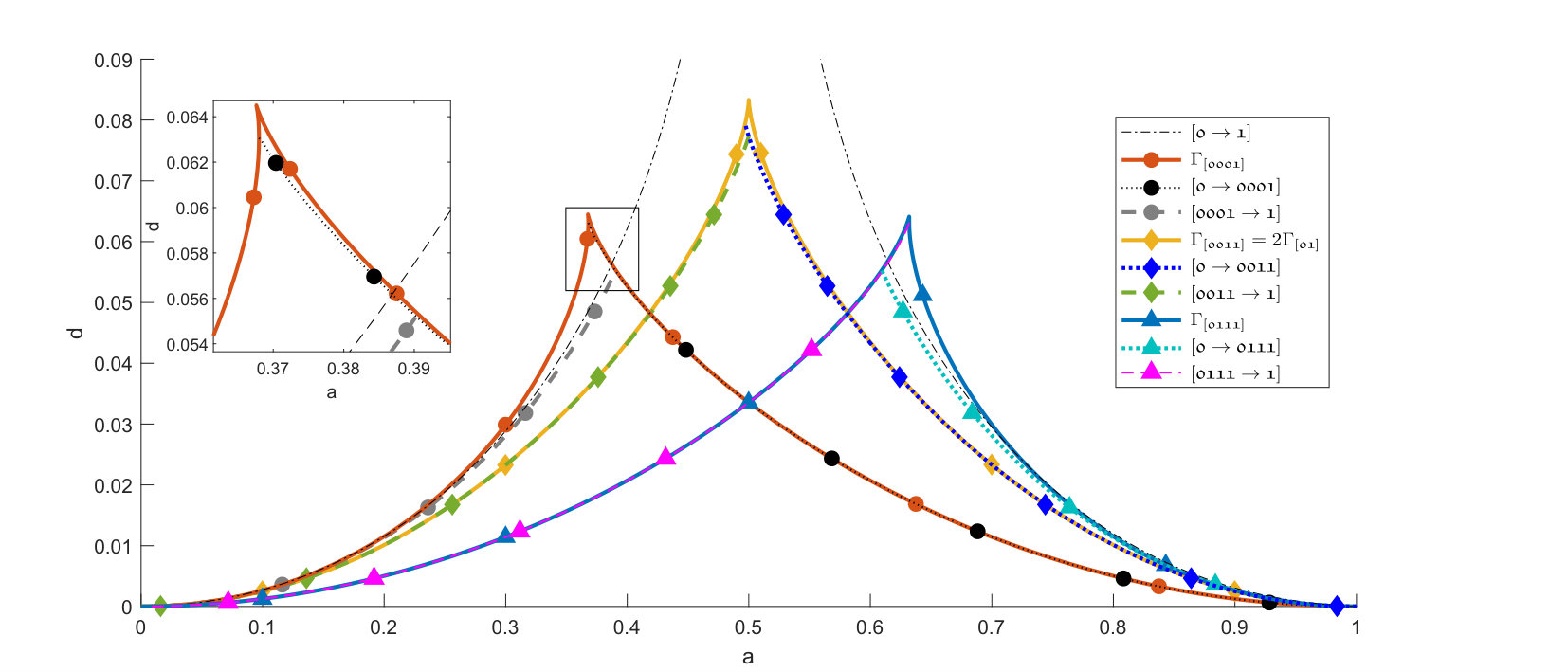 Figure 1
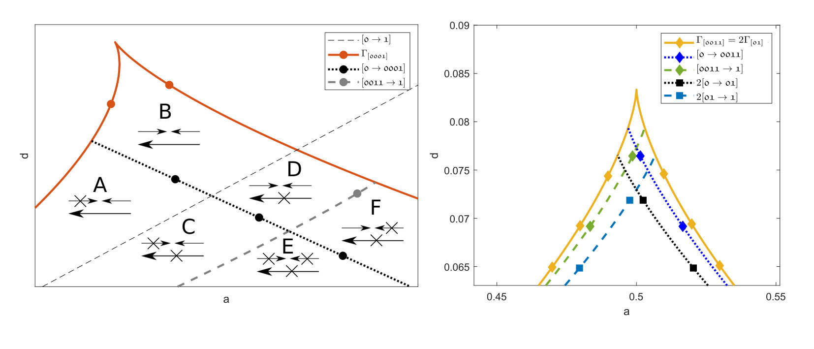 Figure 2
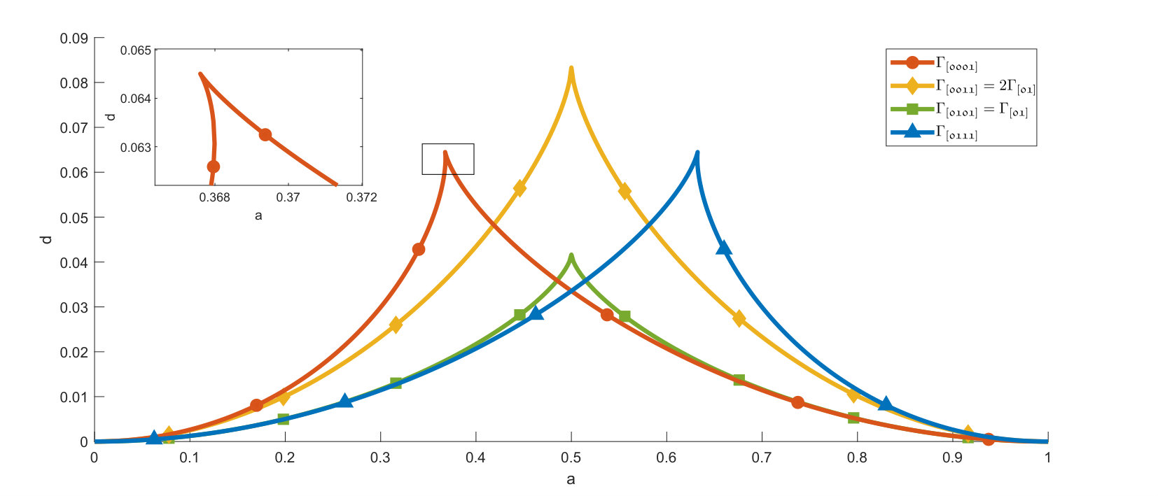 Figure 3
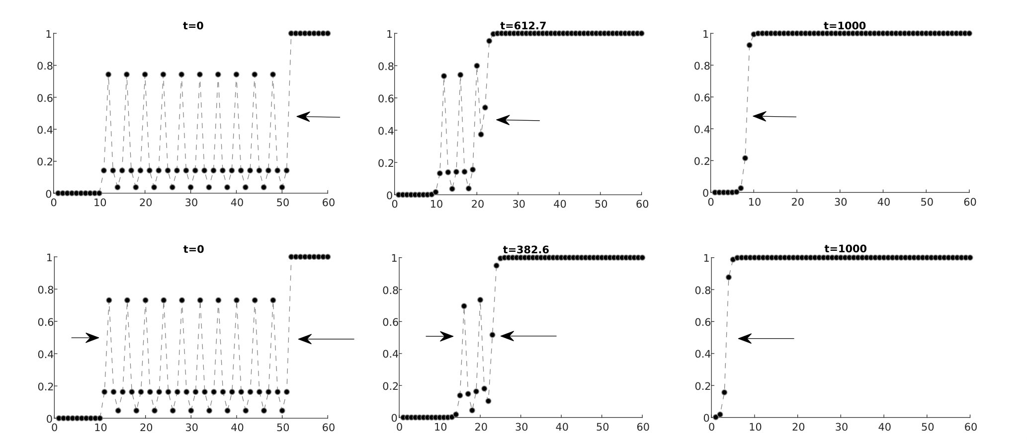 Figure 4
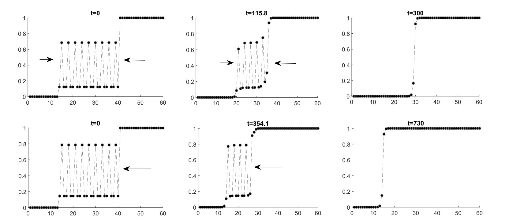 Figure 5
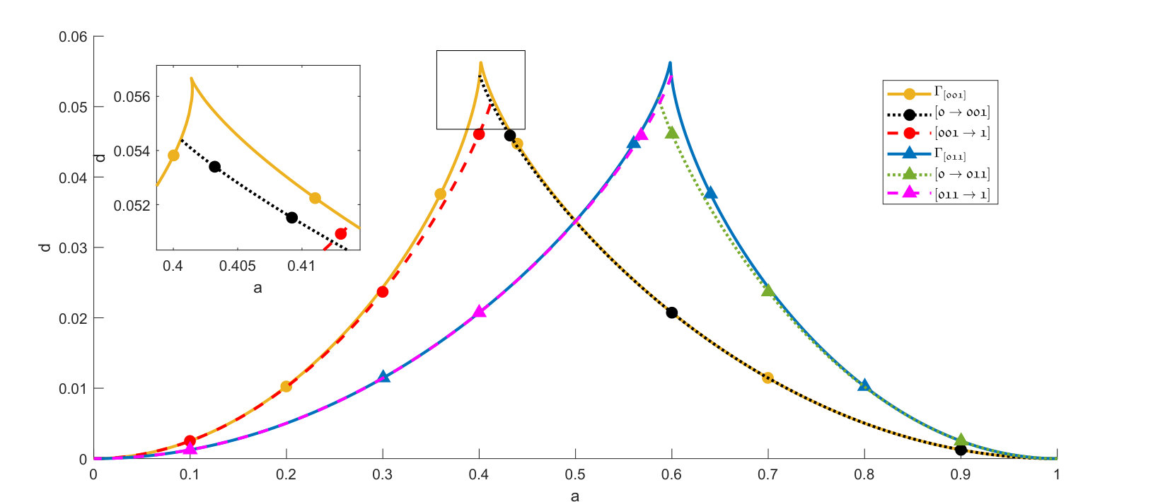 Figure 6
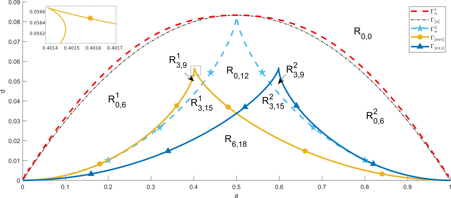 Figure 7
 Figure 8
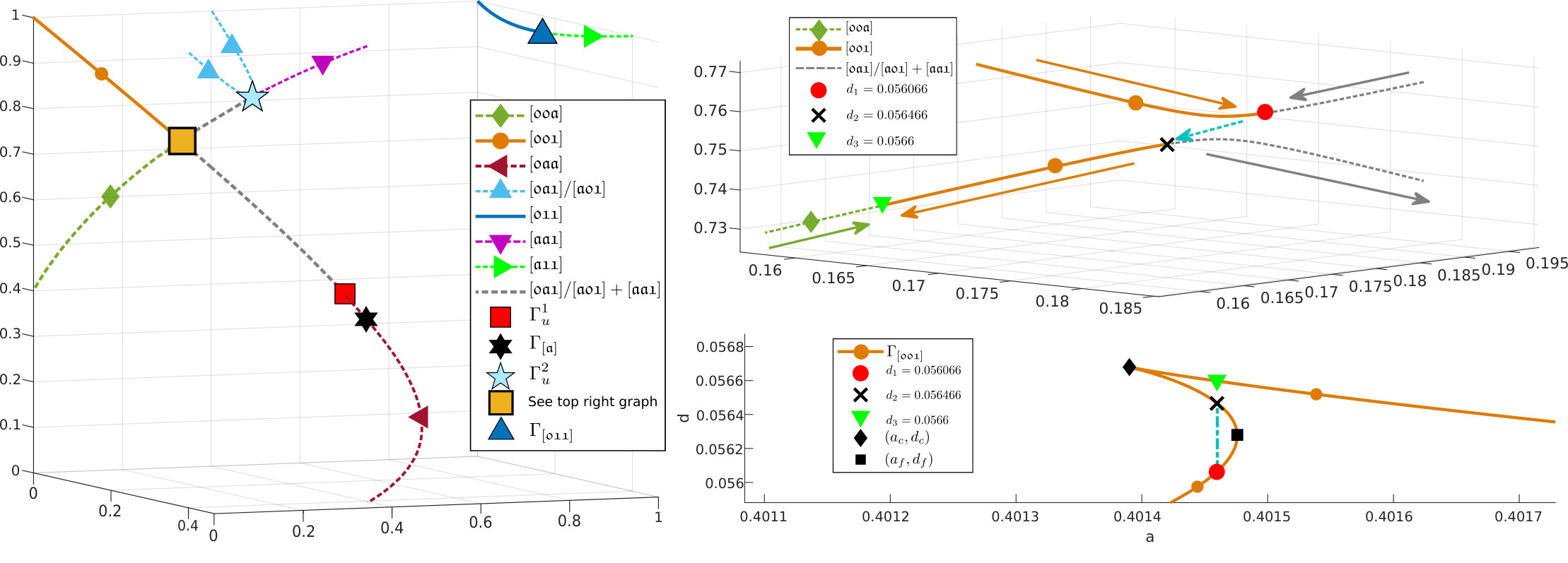 Figure 9
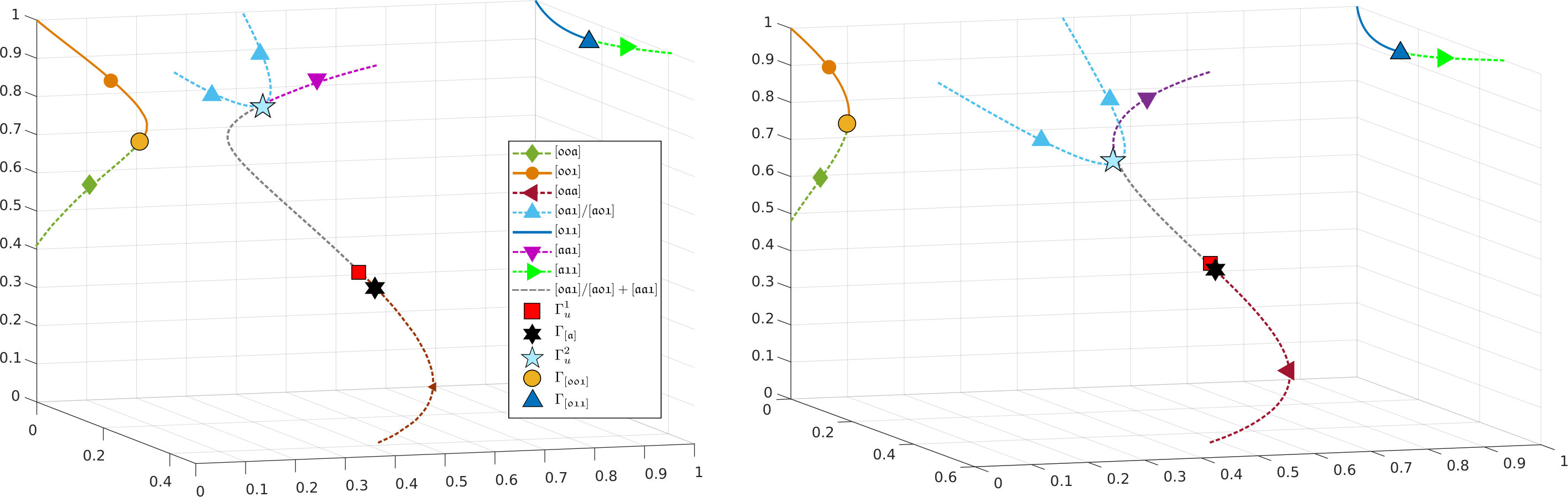 Figure 10
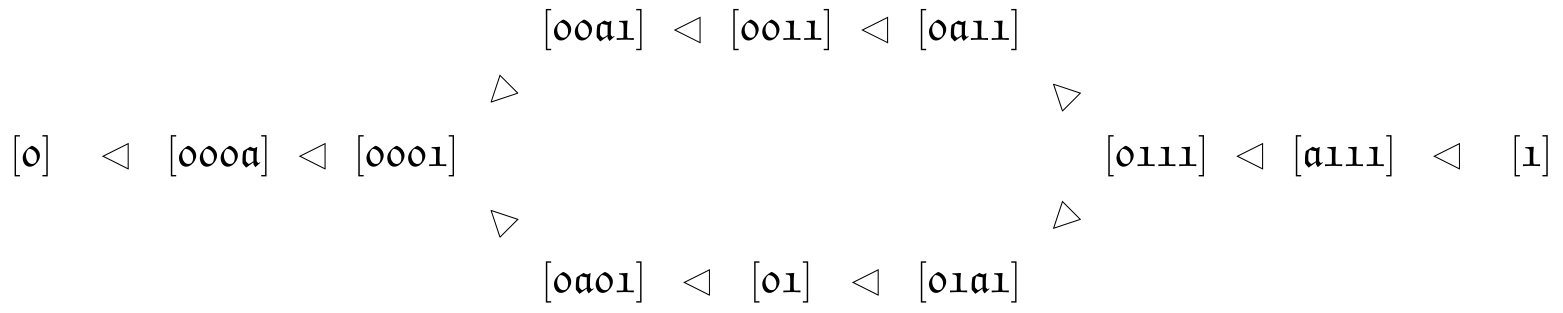 Figure 11
 Figure 12
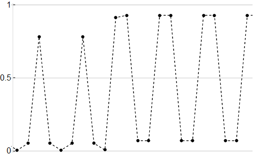 Figure 13
Peer Reviews
No public reviews on file for this paper yet. If you reviewed it on a platform where reviews are public (OpenReview, ICLR, NeurIPS, ICML), you can paste yours below so the community can read it here.
Videos
No videos yet. Explain this paper in a talk, walkthrough, or lecture? Add one.
Taxonomy
TopicsStochastic processes and statistical mechanics · Theoretical and Computational Physics
Multichromatic travelling waves for lattice Nagumo equations
Hermen Jan Hupkes [email protected] Mathematisch Instituut, Universiteit Leiden, P.O. Box 9512, 2300 RA Leiden, The Netherlands
Leonardo Morelli [email protected] Mathematisch Instituut, Universiteit Leiden, P.O. Box 9512, 2300 RA Leiden, The Netherlands
Petr Stehlík corresponding author, [email protected] Department of Mathematics and NTIS, Faculty of Applied Sciences, University of West Bohemia,
Univerzitní 8, 306 14 Plzeň
Czech Republic
Vladimir Švígler [email protected] Department of Mathematics and NTIS, Faculty of Applied Sciences, University of West Bohemia,
Univerzitní 8, 306 14 Plzeň
Czech Republic
Abstract
We discuss multichromatic front solutions to the bistable Nagumo lattice differential equation. Such fronts connect the stable spatially homogeneous equilibria with spatially heterogeneous -periodic equilibria and hence are not monotonic like the standard monochromatic fronts. In contrast to the bichromatic case, our results show that these multichromatic fronts can disappear and reappear as the diffusion coefficient is increased. In addition, these multichromatic waves can travel in parameter regimes where the monochromatic fronts are also free to travel. This leads to intricate collision processes where an incoming multichromatic wave can reverse its direction and turn into a monochromatic wave.
Keywords: reaction-diffusion equations; lattice differential equations; travelling waves; wave collisions.
MSC 2010: 34A33, 37L60, 39A12
1 Introduction
In this paper we are interested in the Nagumo lattice differential equation (LDE)
[TABLE]
posed on the one-dimensional lattice , for small values of the diffusion-coefficient . This so-called anti-continuum regime features spatially periodic equilibria for (1.1) that can serve as buffer zones between regions of space where the homogeneous stable equilibria and dominate the dynamics. Our goal here is to continue the program initiated in [24] where two-periodic patterns and their connection to bichromatic waves were rigorously analyzed.
In particular, we build a classification framework that also allows larger periods to be considered. We also construct so-called multichromatic waves, which connect heterogeneous -periodic rest-states to each other or their homogeneous counterparts and . We numerically analyze these multichromatic waves for and show that they exhibit richer behaviour than the bichromatic versions. Indeed, these multichromatic waves can disappear and reappear as the diffusion is increased. In addition, open sets of parameters exist where monochromatic and multichromatic waves can travel simultaneously. This allows us to explore various new types of wave collisions.
Reaction-diffusion systems
The LDE (1.1) can be seen as the spatial discretization of the Nagumo PDE
[TABLE]
onto a uniform grid with node-spacing . This scalar reaction-diffusion PDE can serve as a highly simplified model to describe the interaction between two species or states (described by and ) that compete for dominance in a spatial domain [1]. It admits a comparison principle and can be equipped with a variational structure [20], but it also has a rich global attractor. As such, it has served as a prototype system to investigate many of the key concepts in the field of pattern formation, such as spreading speeds for compact disturbances [42], the existence and stability of travelling waves [19, 36] and other non-trivial entire solutions [31, 43].
The semi-discrete version (1.1) has served as a playground to investigate the impact of the transition from a spatially continuous to a spatially discrete domain. From a mathematical point of view, interesting questions and complications arise due to the broken translational invariance [28]. From the practical point of view, it is highly desirable to be able to incorporate the natural spatial discreteness present in many physical systems such as myelinated nerve fibres [35], meta-materials [7, 8, 39] and crystals [9, 12].
Monochromatic waves
Substitution of the travelling wave Ansatz into the PDE (1.2) yields the travelling wave ODE
[TABLE]
On the other hand, substitution of the discrete analog into the LDE (1.1) yields the monochromatic wave equation
[TABLE]
which is a functional differential equation of mixed type (MFDE). We use the term monochromatic here to refer to the fact that each spatial index follows the same waveprofile . We are specially interested in waves that connect the two stable equilibria and . In particular, we impose the boundary conditions
[TABLE]
The ODE (1.3) with (1.5) can be analyzed by phase-plane analysis [19] (and even solved explicitly) to yield the existence of solutions that increase monotonically and have . These waves have a large basin of attraction [19] and can be used as building blocks to construct and analyze more complicated solutions [42].
More advanced techniques are required to analyze (1.4), but again it is possible to show that non-decreasing solutions exist [29]. However, it is now a very delicate question to determine whether the uniquely determined wavespeed satisfies or . Indeed, the broken translational invariance causes an energy-barrier that must be overcome before waves are able to travel. As such, there is an open region in the -plane for which holds; see Fig. 10. This pinning phenomenon is generic [2, 6, 15, 16, 21, 26, 27, 30] but not omnipresent [14, 25] in discrete systems and has received considerable attention.
Bichromatic waves
The discrete second derivative allows (1.1) to have a much larger class of equilibrium solutions than the PDE (1.2). For example, two-periodic equilibria of the form
[TABLE]
can be found by solving the two-component system given by
[TABLE]
The variable can be readily eliminated, leading to a ninth-order polynomial equation for the remaining component . For this polynomial has nine roots, leading to two stable and four unstable two-periodic equilibria for (1.1) besides the three spatially homogeneous equilibria .
In [24] we performed a full rigorous analysis of this system, which shows that the number of these two-periodic equilibria decreases as is increased. In particular, there exist two functions defined for so that the two stable patterns and collide with two unstable patterns and disappear as crosses . The remaining two unstable patterns subsequently collide with as crosses , leaving only the three spatially homogeneous equilibria. We emphasize that all these two-periodic equilibria only exist in the region where monochromatic waves are pinned, i.e. .
Based on general results in [10] we showed that for the system (1.1) admits two types of bichromatic waves
[TABLE]
The first class satisfies the lower limits
[TABLE]
and has wavespeed , while the second class satisfies the upper limits
[TABLE]
and has . In [24] we showed that there exist two thresholds
[TABLE]
so that in fact respectively holds as is increased above these thresholds. In addition, for all one or both of the inequalities in (1.11) is strict, indicating the presence of one or more travelling bichromatic waves for sufficiently close to .
Numerical results indicate that these two types of bichromatic waves can be glued together via an intermediate buffer zone that displays the two-periodic pattern . This buffer zone is consumed as the waves move towards each other and eventually collide to form a trapped monochromatic wave; see Figure 8 for the trichromatic analogue.
Bichromatic waves have also been found in several other spatially discrete settings. The results in [5, 40] apply to an anti-diffusion version of (1.1) where . This can reformulated as a two-component problem with positive alternating diffusion coefficients, allowing the general results in [10] to be applied. Several versions of the two-periodic FPU problem are considered in [17, 18, 23]. Using a different palette of techniques, the authors obtain so-called nanopteron solutions, which can have small high-frequency oscillations in their tails. Finally, the two-periodic FitzHugh-Nagumo problem was considered in [37] using a modified spectral-convergence argument.
Multichromatic waves
The main purpose of the present paper is to illustrate the novel behaviour that arises for (1.1) when considering wave connections to/from stable -periodic patterns with . Our two main conclusions are that the monotonicity properties described above are no longer valid and that travelling multichromatic waves can co-exist with travelling monochromatic waves. In particular, travelling multichromatic waves can appear, disappear and reappear as is increased and can collide with other multichromatic waves to form travelling monochromatic waves.
Since the degree of the polynomial that governs the -periodic equilibria is given by , it is essential to develop an appropriate classification system to keep track of all the roots and their ordering properties. We develop such a system in this paper, using words from the set to track roots that bifurcate off the corresponding sequence of zeroes of the cubic at . The lack of monotonicity with respect to leads to complications and forces us to allow both parameters to vary when tracking roots of a related algebraic problem, unlike in [24]. Although the general theory in [10] also applies to our setting, it is still a challenge to check the conditions in a systematic fashion.
Wave collisions
Understanding the interaction between waves is an important topic that is attracting considerable attention, primarily in the spatially continuous setting at present. The so-called weak interaction regime where the waves are far apart is relatively well-understood; see e.g. the exit manifold developed by Wright and Hoffman [22] for the discrete setting and the numerous studies on renormalization techniques for the continuous setting [3, 13, 41].
However, at present there is no general theory to understand strong interactions, where the core of the waves approach each other and deform significantly. Early numerical results by Nishiura and coworkers [33] for the Gray-Scott and a three-component FitzHugh-Nagumo system suggest that the fate of colliding waves (annihilation, combination or scattering) is related to the properties of a special class of unstable solutions called separators. Even the internal dynamics of a single pulse under the influence of essential spectrum (a proxy for the advance of a second wave) can be highly complicated, see e.g. [11] for the (partial) unfolding of a butterfly catastrophe.
Naturally, more information can be obtained in the presence of a comparison principle. Indeed, for the PDE (1.2) one can show that monostable waves can merge to form a bistable wave [31] and that counterpropagating waves can annihilate [32, 43]. If one modifies the nonlinearity to allow more zero-crossings, one can stack waves that connect a chain of equilibria to form so-called propagating terraces [34].
We emphasize that the collisions described in this paper are far richer than those described above for (1.2). This is a direct consequence of the delicate structure of the set of equilibria for (1.1). By exploiting the comparison principle, our hope is that this system can serve as a playground for generating and understanding complicated collision processes.
Organization
In §2 we discuss the algebraic problem that -periodic equilibria must satisfy, develop a naming scheme for its roots and formulate a result concerning the existence of travelling waves. In §3 we discuss trichromatic waves and focus on the fact that for certain values of three-periodic stable equilibria can disappear and reappear as the diffusion parameter is increased. We move on to quadrichromatic waves in §4, highlighting the fact that quadrichromatic and monochromatic waves can travel simultaneously in certain parameter regions. This allows us to study various types of wave collisions. Finally, in §5 we prove our main result Theorem 2.2, which establishes the existence of multichromatic waves.
Acknowledgments
HJH acknowledges support from the Netherlands Organization for Scientific Research (NWO) (grant 639.032.612). LM acknowledges support from the Netherlands Organization for Scientific Research (NWO) (grant 613.001.304). PS acknowledges the support of the project LO1506 of the Czech Ministry of Education, Youth and Sports under the program NPU I. The authors are grateful to Antonín Slavík for his comments.
2 Multichromatic Root Naming and Ordering
The main focus of this paper is the Nagumo lattice differential equation (LDE)
[TABLE]
in which the parameters are taken from the half-strip
[TABLE]
and the nonlinearity is given by the cubic
[TABLE]
Our results focus on -periodic stationary solutions to (2.1) and the waves that connect them.
In §2.1 we develop a naming system that allows us to partially classify these stationary solutions in an intuitive fashion. We proceed in §2.2 by formulating a result for the existence of waves that uses our naming system to decide which equilibria can be connected. Finally, equivalence classes for these waves are introduced in §2.3 by exploiting the symmetries present in (2.1).
2.1 Equilibrium types
We will write -periodic equilibria for the LDE (2.1) in the form
[TABLE]
for some vector , where we let the modulo operator take values in
[TABLE]
We remark that can be interpreted as a solution of the Nagumo equation posed on a cyclic graph of length ; see [38]. Taking and introducing the nonlinear mapping
[TABLE]
we see that any such equilibrium must satisfy .
For any and , it is easy to see that and to confirm that the diagonal matrix
[TABLE]
has non-zero entries. In particular, the implicit function theorem implies that each of these roots is part of a smooth one-parameter family of roots that exists whenever is small. In fact, one can track the location of each of these roots as is increased, up until the point where the root in question disappears by colliding with another root. This procedure forms the heart of the naming scheme that we develop here, which will allow us to refer to different types of roots in an efficient manner.
In particular, we set out to label solutions of the equation with words taken from the set . We emphasize that we are using the fixed symbol as placeholder for the parameter , which is allowed to vary. Indeed, for any we introduce the vector by writing
[TABLE]
Definition 2.1**.**
Consider a word together with a triplet
[TABLE]
Then we say that is an equilibrium of type if there exists a -smooth curve
[TABLE]
so that we have
[TABLE]
together with
[TABLE]
for all .
We note that substituting in (2.12) shows that indeed , justifying the terminology of an equilibrium. In addition, the second requirement in (2.12) allows us to apply the implicit function theorem to conclude that also has equilibria of type for all pairs sufficiently close to . In particular, these observations allow us to introduce the pathwise connected set
[TABLE]
which is open in the half-strip .
We now impose the following conditions on the structure of these sets . The second of these basically states that the interior of the curve (2.10) can be perturbed freely within without changing the value of the equilibrium .
For any two words the intersection is connected.
Consider any word and any , together with a pair of curves
[TABLE]
that have
[TABLE]
Then there exist unique functions
[TABLE]
so that the triplets and both satisfy (2.12) for all , together with the identities
[TABLE]
At first glance, the condition appears to be rather cumbersome to verify in practice. To make this more feasible, it is useful to introduce the set
[TABLE]
which by continuity is a closed subset of . Let us assume that consists of a finite number of components that are open in and simply connected. On account of a global implicit function theorem [4, Thm. 3], there exist non-negative integers together with smooth functions
[TABLE]
so that for each . In addition, whenever and every solution with can be written in this way.
In this setting, can be verified by checking which of these functions can be connected continuously through the boundaries of adjacent components. Indeed, is satisfied if there is no sequence of connections that starts in and ends in for some and some pair .
In any case, writing for the component of that contains the horizontal segment , can always be achieved if one replaces by subsets of the form
[TABLE]
However, we emphasize that appears to be valid without this artificial restriction for the regions that we have numerically computed in this paper.
Corollary 2.1**.**
Fix an integer and suppose that and both hold. Then for any word there is a smooth function so that is the unique equilibrium of type for the system for all . In addition, whenever for two distinct words we have
[TABLE]
Proof.
The first statement is a consequence of and the implicit function theorem. For the second statement, let us argue by contradiction and assume that both vectors in (2.21) are equal to . Condition allows us to pick a path from to that lies entirely within . Applying shows that can be continued as an equilibrium along this path back to both and . However, the implicit function theorem implies that this continuation should be unique. ∎
We emphasize that our classification scheme only track roots until the first time the associated Jacobian becomes singular and the implicit function theorem can no longer be applied. We will encounter several different types of behaviour at such points. It is possible for two roots to collide and become complex and sometimes even recombine at ‘later’ parameter values. We will also encounter multi-root collisions where one or more roots survive the collision process. In such cases, we often use an ad-hoc naming system, where we label the emerging branch by reusing or combining the types of the original colliding branches.
2.2 Waves
In this section we focus on wave solutions to (2.1) that connect the -periodic stationary solutions investigated in the previous section. These so-called multichromatic waves can be written as
[TABLE]
for some wavespeed and -valued waveprofile
[TABLE]
that satisfies the boundary conditions
[TABLE]
for some pair of words ; see Corollary 2.1.
Substituting this Ansatz into (2.1) yields the traveling wave functional differential equation
[TABLE]
which has positive coefficients on all shifted terms and also has diagonal nonlinearities. This system hence fits into the framework developed in [10], provided that the assumptions pertaining to the boundary conditions (2.24) can also be validated.
This is in fact the key question that we address in our main result below. This result requires the following assumption, which states that our root tracking scheme captures all (marginally) stable111 We use the eigenvalues of the matrix to characterize the stability of . Using the comparison principle this can be easily transferred to the full LDE (1.1).
-periodic equilibria of the LDE. In particular, the types of these equilibria correspond with words from the stable subset .
- (HS)
Recall the definitions (2.2) and (2.18) and suppose that for some and . Suppose furthermore that all eigenvalues of satisfy . Then we have222 If this identity should be interpreted as a limit. for some and .
Theorem 2.2** (see §5).**
Fix an integer and assume that , and all hold. Consider two distinct words with and pick with . Suppose furthermore that one of the following conditions holds.
- (a)
The words and differ at precisely one location.
- (b)
For each that satisfies we have .
Then there exists a unique for which the travelling system (2.25) admits a solution that satisfies the boundary conditions
[TABLE]
If , then is unique up to translation and each component is strictly increasing.
2.3 Symmetries
There are a number of useful symmetries present in the equilibrium equation and the travelling wave MFDE (2.25). We explore three important transformations here that significantly reduce the number of cases that need to be considered.
We first note that the identity implies that
[TABLE]
holds for all , with . In order to exploit this, we pick and write for the ‘inverted’ word
[TABLE]
The identity (2.27) directly implies the reflection relation
[TABLE]
together with
[TABLE]
We proceed by introducing the coordinate-shifts and reflection that act as
[TABLE]
It is easy to verify that the identity implies that also
[TABLE]
In addition, when is a solution to the travelling wave MFDE (2.25), the same holds for the coordinate-shifted pair and the reflected version with
[TABLE]
These identities are all consequence of the invariance of the Nagumo LDE (2.1) under the transformations and .
Our choice to only consider waves where breaks the reflection invariance (2.33), which allows us to focus solely on the symmetry caused by the coordinate shifts . In particular, for any word , we write
[TABLE]
In addition, we introduce the shorthand notation
[TABLE]
to refer to all the roots in the corresponding equivalence class, which are defined for .
Note that we are hence treating and as separate classes, even though they correspond with equivalent equilibria of . Interestingly enough, when restricting attention to the alphabet , this distinction only plays a role for . For example, is not shift-related to its reflection , but all shorter binary sequences are.
Whenever we are referring to an equivalence class of roots, we will use the word that is the smallest in the lexicographical333For ordering purposes we assume that holds.
sense (the so-called Lyndon word) as a class representative. For example, is the Lyndon word for the class
[TABLE]
We note that shorter words with a length that divides can also be interpreted as a word of length by periodic extension. For example, we write
[TABLE]
For any pair with , we will use the shorthand notation to refer to any pair that satisfies the travelling wave MFDE (2.25) together with the boundary conditions (2.26). The observations above show that then corresponds with the pair .
In order to refer to an equivalence class of wave solutions, we pick and introduce the notation
[TABLE]
Here we always take to be the Lyndon representative for its equivalence class, but we emphasize that cannot always be chosen in this way. For example,
[TABLE]
refers to a different set of waves than
[TABLE]
Naturally, this distinction disappears when considering waves that connect to or from one of the monochromatic states and .
3 Trichromatic waves
In this section we apply our results to the trichromatic case . As in the bichromatic case considered in [24], we observe that stable -periodic equilibria can only exist inside the parameter region where the monochromatic wave is pinned. The novel behaviour as compared to the bichromatic case is that there exist intervals of the parameter in which the number of (stable) equilibria can actually increase as is increased (e.g., for , see Figures 2 and 4). In addition, for values of in these intervals, there are two disjoint intervals of parameters for which travelling trichromatic waves exist that connect the homogeneous states and to a stable -periodic equilibrium. Similarly, for a fixed , the number of (stable) equilibria can increase as is increased (e.g., for , see Figure 2).
3.1 Equilibria
Trichromatic equilibria for (2.1) correspond to roots of the nonlinear function
[TABLE]
Inspection of this system shows that one component can be removed if one enforces either , or .
In Figure 2 we numerically computed the critical set defined in (2.18) by searching for roots of the augmented system
[TABLE]
The results show that can be decomposed into 5 piecewise-smooth curves that we label as , , , and . The labels of the form imply that . We emphasize that this naming scheme is ambiguous by its very nature. Indeed, collisions between roots occur precisely on these curves, which also intersect each other.
These 5 curves divide the remaining parameter space into 11 open and simply connected components. Ignoring the three homogeneous roots444 In the current trichromatic context, these roots are given by , and . , and , the bottom region contains stable roots and unstable roots. The stable roots are represented by the equivalence classes and , while all the remaining equivalence classes generate the unstable roots.
In the discussion below we indicate how this configuration changes as each of the critical curves is crossed. For now, we recall the identity (2.27), which explains the reflection symmetry through the line and allows us to focus on the case .
The threshold
The first threshold that is encountered when increasing for is the curve . Here the stable roots collide with the unstable roots , after which both branches disappear. This collision is visible in Figures 3, 4 and 5.
In order to find an expansion for this threshold near the corner , we exploit the observations above which allow us to consider equilibria close to for which the second and third components are equal. In particular, we construct solutions to the problem
[TABLE]
for which is small. The resulting system has a structure that is very similar to that encountered in [24], allowing us to follow the exact same procedure to unfold the saddle node bifurcations. In particular, viewing locally as the graph of the function , we obtain the expansion
[TABLE]
together with
[TABLE]
The threshold
This curve features the triple collision of the unstable branches , and when . One unstable branch of roots emerges from this collision. This collision is visible in Figures 3, 4 and 5.
The threshold
The important feature of this curve is that cannot be expressed as a function of . Indeed, the function
[TABLE]
has the (numerically computed) roots
[TABLE]
which correspond with a cusp respectively fold point for the curve ; see Figures 2 and 4.
When , the root hits the branch spawned by the collision and disappears; see Figure 3. On the other hand, for the root hits ; see Figure 5. This corresponds with the scenario described above for after applying the swap.
The intermediate case is illustrated in Figure 4. In this case the root again hits the branch spawned by the collision and disappears, but this pair reappears and splits off from each other after crosses the threshold a second time. The stable branch of this pair collides with and disappears when crosses for the third and final time, while the unstable branch emerges as the survivor of the full triple crossing process.
The black star and green triangle in Figure 4 overlap when , in which case the branch has a triple root at the critical value . On the other hand, the black star and red circle in this figure overlap when , in which case the branch and the branch spawned by the collision can be said to bounce off each other at .
In order to find an expansion for this threshold near the corner , we now look for solutions to
[TABLE]
for which is small. Viewing locally as the graph of the function , we may again use the same procedure as in [24] to obtain the expansion
[TABLE]
together with
[TABLE]
The threshold
This curve is characterized by the relation , which can be explicitly solved to yield . As shown in Figure 3, the three branches of roots contained in the equivalence class all pass through at and survive the collision.
The threshold
On this threshold the unstable branch that survived the and collisions hits the branch that passed through ; see Figures 3, 4, 5. Above this threshold the only remaining equilibria are the homogeneous states and .
The critical case
The right panel in Figure 5 describes the situation just before reaches the critical value . Upon increasing through this value, the collisions at and both cross through the center at and , transitioning to occur on the branch.
3.2 Wave Connections
Our numerical results strongly suggest that , and are satisfied, allowing us to apply the results in §2. Figure 7 represents the equivalence classes of wave connections between neighbouring words. We note that we are not drawing an edge from because this is not a Lyndon word.
We recall that Theorem 2.2 does not provide any information about the speed of the travelling wave. We therefore resorted to numerics to find parameter values where for the waves discussed in the diagram above. This was done by connecting the two endstates with a profile and letting this initial profile evolve under the flow of (2.1). Exploiting the stability of the moving waves, one can test whether by determining whether movement ceases after an initial transient period.
For the and connections we were not able to find any regions where . However, in Figure 6 we can observe the numerically computed minimum threshold for where we in fact have for the waves that connect to and from the homogeneous states and . Notice that both types of waves have non-zero speed in the region around the fold and cusp points of . This indicates that travelling waves can appear and disappear twice as the diffusion coefficient is increased, which does not happen in the bichromatic case.
In Figure 8 we give snapshots of the collision process that occurs as a wave collides with a wave. In both cases an intermediate buffer-zone consisting of the trichromatic state is consumed by one (or both) of the incoming trichromatic waves, leading eventually to a pinned monochromatic wave. This type of collision can also be observed in the bichromatic setting.
4 Quadrichromatic waves
In this section we discuss the quadrichromatic case . As in the trichromatic case, stable -periodic equilibria can disappear and reappear as is increased for a fixed . The novel behaviour in this setting is that travelling quadrichromatic waves can co-exist with travelling monochromatic waves for an open set of parameters . This allows several new types of collisions to occur. For example, two incoming connections with intermediate quadrichromatic states can collide to form a monochromatic travelling wave.
4.1 Equilibria
The relevant nonlinearity that governs quadrichromatic equilibria to (2.1) is now given by
[TABLE]
Inspecting this system shows that one component can be removed by enforcing either or . Of course, this problem reduces to the bichromatic case if both these identities are enforced. On the other hand, if one takes
[TABLE]
the system reduces to
[TABLE]
This again corresponds to the bichromatic case but now with the halved diffusion coefficient .
In Figure 9 we display several numerically computed curves in the critical set that correspond with the upper boundaries of the sets . For visual clarity, we only consider the words
[TABLE]
which correspond with the stable non-homogeneous equilibria for .
The curves and again contain cusp and fold points. However, all four curves can locally be described as a graph near the corner . We now set out to compute the first two terms in the asymptotic expansion of each of these curves.
The threshold
In view of the symmetries discussed above we consider solutions where the second and fourth component are equal. In particular, we consider the problem
[TABLE]
which can be written as
[TABLE]
with
[TABLE]
Notice that and feature terms of order respectively , which corresponds with the fact that the root is simple when . In addition, is independent of . Setting hence allows us to write , which can be substituted into to yield . Plugging these expressions into by writing
[TABLE]
we find
[TABLE]
This allows us to uncover the saddle-node bifurcations in a fashion analogous to [24]. In particular, we obtain the expansion
[TABLE]
together with
[TABLE]
The threshold
The discussion above implies that this threshold is identical to the corresponding threshold for the bichromatic case . We can hence copy the results from [24, Prop 3.6] and write
[TABLE]
together with
[TABLE]
The threshold
The identity (4.3) allows us to write
[TABLE]
In addition, we can reuse the expressions (4.13) to find
[TABLE]
The threshold
The symmetries discussed above allow us to consider solutions where the first and third component are equal. In particular, we consider the problem
[TABLE]
which can be written as
[TABLE]
with
[TABLE]
Notice that features a term of order and is independent of . In fact, it is very similar to [24, Eq. (3.30)], which allows us to write
[TABLE]
However features O\big{(}(a+d)y\big{)} terms, which prevents us from expressing in terms of as before. This corresponds with the fact that the root is double at . On the other hand, setting and introducing the scalings
[TABLE]
does allow us to write
[TABLE]
Substituting these expressions into , we write
[TABLE]
and find
[TABLE]
The saddle-node bifurcations can now be unfolded by examining the terms in this equation using the procedure in [24]. In particular, we find
[TABLE]
together with
[TABLE]
The main point of interest here is that contains a cubic term. In fact, our expansion here agrees with the expansion of the formula [27, Eq. (5.1)], which provides a (non-sharp) upper bound for the values of where monochromatic waves are pinned. As indicated in Figure 10, our numerical results confirm that intersects the region in space where monochromatic waves can travel.
4.2 Wave connections
As in the trichromatic case, a visual inspection confirms that assumptions , and are satisfied. The connections predicted by Theorem 2.2 are depicted in Figure 7. In Figure 10 we provide the numerically computed minimal values for for which the waves connecting to and from the spatially homogeneous equilibria and have a non-zero speed. The novel feature here is that there is overlap with the region where the monochromatic wave has non-zero speed. This allows for situations where the end-product of a collision between two quadrichromatic wave is no longer a pinned monochromatic wave but in fact a travelling monochromatic wave.
The parameter regions where various types of collisions can occur are described in Figure 11. Types - closely resemble those encountered in the bichromatic and trichromatic cases. Types and are new and indeed feature travelling monochromatic end-products. Two examples with snapshots of such collisions are provided in Figure 12.
5 Proof of Theorem 2.2
Here we provide the proof of our main result, which allows us to establish the existence of wave connections between equilibria by simply comparing their types.
We first show that a pair of distinct ordered stationary solutions cannot have two equal components. Throughout this section we assume that expressions such as or should be evaluated within the modulo arithmetic on indices .
Lemma 5.1**.**
Assume that satisfy for some pair and . Assume furthermore that and that for some . Then in fact .
Proof.
Since we have
[TABLE]
which implies that
[TABLE]
Since and we obtain and . This argument can subsequently be repeated a number of times to yield . ∎
The main ingredient in our proof of Theorem 2.2 is that the ordering of any pair of words from the full set and the stable subset is preserved for the equilibria that have the corresponding types. For example, for we have the partial ordering
whereby each connection in this diagram indicates that whenever with .
Lemma 5.2**.**
Assume that and are satisfied and consider a distinct pair that admits the ordering . Suppose furthermore that at least one of these two words is contained in . Then for any we have the strict component-wise inequality
[TABLE]
Proof.
Fixing , we note that and allow us to pick a curve
[TABLE]
so that we have
[TABLE]
while the inclusion
[TABLE]
and the identities
[TABLE]
all hold for . By slightly modifying the path and picking a small , we can also ensure that and for all .
Upon introducing the graph Laplacian and the nonlinearity that act as
[TABLE]
we see that
[TABLE]
for small and . Taking implicit derivatives of (5.9), we find
[TABLE]
in which we have defined
[TABLE]
for , setting this expression to zero for .
For any index we define the quantity
[TABLE]
which measures the distance to the closest index where and are unequal. We now claim that for any we have
[TABLE]
if , with the inequality being strict if and only if . For this is obvious. Assuming this holds for , consider any index with . Our alphabet assumption implies that
[TABLE]
which implies that the -component of the two diagonal matrices D\Psi\big{(}\mathrm{v}_{A}(0)\big{)} and D\Psi\big{(}\mathrm{v}_{B}(0)\big{)} are strictly negative; see (2.7). In addition, our induction hypothesis implies that
[TABLE]
By definition, we have
[TABLE]
In addition, we have if and only if or holds. Our induction hypothesis hence implies
[TABLE]
with strict inequality if and only if . Our claim now follows immediately from (5.10).
The argument above shows that for all . If (5.3) fails to hold, this hence means that there exists for which , with also \big{(}\mathrm{v}_{A}(t_{*})\big{)}_{i}=\big{(}\mathrm{v}_{B}(t_{*})\big{)}_{i} for some . Lemma 5.1 now implies and hence
[TABLE]
which violates Corollary 2.1. ∎
By combining Lemma’s 5.1 and 5.2 we can control all the (marginally) stable equilibria in the box . This allows us to finally prove our main result.
Proof of Theorem 2.2.
Pick any distinct pair with and any with . Lemma 5.2 implies that the cuboid
[TABLE]
has non-empty volume. In addition, for any that does not satisfy and for which , we have on account of Lemma 5.1, the connectedness of and continuity considerations.
In view of (HS), all equilibria inside the cube besides the two corner points hence have a strictly positive eigenvalue. The existence of the wave now follows from [10, Thm. 6]. ∎
The reference list from the paper itself. Each links out to its DOI / PubMed record.
- 1[1] D. G. Aronson and H. F. Weinberger (1975), Nonlinear diffusion in population genetics, combustion, and nerve pulse propagation. In: Partial differential equations and related topics . Springer, pp. 5–49.
- 2[2] P. W. Bates and A. Chmaj (1999), A Discrete Convolution Model for Phase Transitions. Arch. Rational Mech. Anal. 150 , 281–305.
- 3[3] T. Bellsky, A. Doelman, T. J. Kaper and K. Promislow (2013), Adiabatic stability under semi-strong interactions: the weakly damped regime. Indiana University Mathematics Journal pp. 1809–1859.
- 4[4] J. Blot (1991), On global implicit functions. Nonlinear Analysis: Theory, Methods & Applications 17 (10), 947–959.
- 5[5] M. Brucal-Hallare and E. S. Van Vleck (2011), Traveling Wavefronts in an Antidiffusion Lattice Nagumo Model. SIAM J. Appl. Dyn. Syst. 10 , 921–959.
- 6[6] J. W. Cahn, J. Mallet-Paret and E. S. Van Vleck (1999), Traveling Wave Solutions for Systems of ODE’s on a Two-Dimensional Spatial Lattice. SIAM J. Appl. Math. 59 , 455–493.
- 7[7] J. W. Cahn and A. Novick-Cohen (1994), Evolution Equations for Phase Separation and Ordering in Binary Alloys. J. Stat. Phys. 76 , 877–909.
- 8[8] J. W. Cahn and E. S. Van Vleck (1999), On the Co-existence and Stability of Trijunctions and Quadrijunctions in a Simple Model. Acta Materialia 47 , 4627–4639.