Schr\"odinger operators with Coulomb-like potentials
Yuriy Golovaty

TL;DR
This paper investigates how one-dimensional Schrödinger operators with Coulomb-like potentials behave under regularization, revealing their limit interactions and constructing approximations for Coulomb potentials with different boundary behaviors.
Contribution
It characterizes the norm resolvent limits of Schrödinger operators with Coulomb-like potentials and constructs explicit $L^ abla( ext{R})$-approximations for these potentials.
Findings
Limits depend on regularization method and zero-energy resonances.
All possible limit point interactions are classified.
Constructed explicit $L^ abla( ext{R})$-approximations for Coulomb potentials.
Abstract
We study the convergence of 1D Schr\"odinger ope\-rators with the potentials which are regularizations of a class of pseudo-potentials having in particular the form The limit behaviour of in the norm resolvent topology, as , essentially depends on a way of regularization of the Coulomb potential and the existence of zero-energy resonances for -like potential. All possible limits are described in terms of point interactions at the origin. As a consequence of the convergence results, different kinds of -approximations to the even and odd Coulomb potentials, both penetrable and impenetrable in the limit, are constructed.
Click any figure to enlarge with its caption.
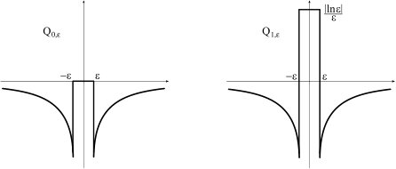 Figure 1
 Figure 2
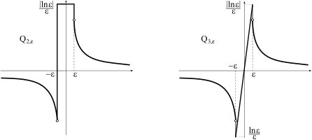 Figure 3
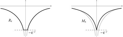 Figure 4
Peer Reviews
No public reviews on file for this paper yet. If you reviewed it on a platform where reviews are public (OpenReview, ICLR, NeurIPS, ICML), you can paste yours below so the community can read it here.
Videos
No videos yet. Explain this paper in a talk, walkthrough, or lecture? Add one.
1-D Schrödinger operators with Coulomb-like potentials
Yuriy Golovaty
Department of Mechanics and Mathematics, Ivan Franko National University of Lviv
1 Universytetska str., 79000 Lviv, Ukraine
Abstract.
We study the convergence of 1D Schrödinger operators with the potentials which are regularizations of a class of pseudo-potentials having in particular the form
[TABLE]
The limit behaviour of in the norm resolvent topology, as , essentially depends on a way of regularization of the Coulomb potential and the existence of zero-energy resonances for -like potential. All possible limits are described in terms of point interactions at the origin. As a consequence of the convergence results, different kinds of -approximations to the even and odd Coulomb potentials, both penetrable and impenetrable in the limit, are constructed.
Key words and phrases:
1D Schrödinger operator, Coulomb potential, one-dimensional hydrogen atom, -potential, scattering problem, penetrability of potential, point interaction
2000 Mathematics Subject Classification:
Primary 34L40, 34B09; Secondary 81Q10
1. Introduction and main results
One-dimensional Schrödinger operators with the Coulomb potentials, the structure of their spectra and the question of penetrability of the Coulomb potentials have been the subject of several mathematical discussions [8, 9, 10], [11, 12, 13, 14], starting with the work of Loudon [1]. These studies are related to the one-dimensional models of the hydrogen atom
[TABLE]
Since the potentials have singularities at the origin, the first derivative of wave function also has in general singularities as , and therefore the wave function should be subject to some additional conditions at . For these formal differential expressions, mathematics gives a large enough set of the boundary conditions associated with self-adjoint operators in [11, 15, 16]. The main issue here is a physically motivated choice of such conditions. We noticed that this problem has many common features with the problem of -potential [17, 18, 19, 20, 21, 22, 23, 24]. First of all, both the Coulomb potential and the -potential are very sensitive to a way of their regularization. From a physical point of view, this means that there is no unique one-dimensional model of the hydrogen atom described by the pseudo-Hamiltonians in (1.1). However there are many different quantum systems with the Coulomb-like potentials that exhibit different physical properties.
We study the norm resolvent convergence of Hamiltonians with the Coulomb-like potentials perturbed by localized singular potentials. Assume that real-valued function is locally integrable outside the origin and has an interior singularity at , namely
[TABLE]
for some real constants , and . We also suppose that is bounded from below if . Set
[TABLE]
where is a function belonging to . Also let and be real-valued, measurable and bounded functions with compact supports. In additional, we suppose that their supports are contained in interval . We study the convergence of Schrödinger operators
[TABLE]
as the positive parameter tends to zero. We hereafter interpret and as -like and -like potentials respectively, because
[TABLE]
in the sense of distributions as , provided is a function of zero-mean. In general, the potentials of diverge, because we do not assume that .
Before stating our main result we introduce some notation. We say that the Schrödinger operator possesses a zero-energy resonance if there exists a non-trivial solution of the equation that is bounded on the whole line. We call the half-bound state. We will also simply say that the potential is resonant and it possesses a half-bound state . We set
[TABLE]
where . These limits exist, because the half-bound state is constant outside the support of as a bounded solution of equation . Moreover, both the values are different from zero. Since a half-bound state is defined up to a scalar factor, we fix half-bound state so that
[TABLE]
Let us set
[TABLE]
We also introduce the spaces
[TABLE]
and denote by the space of -functions such that . Here denotes the set of functions on which are absolutely continuous on every compact subset of . Note that the first derivative of is in general undefined at the origin and has a logarithmic singularity at this point [11, 8, 12].
We say self-adjoint operators converge as in the norm resolvent sense if the resolvents converge in the uniform operator topology for all .
Our main result reads as follows.
Theorem 1**.**
The operator family given by (1.4) converges as in the norm resolvent sense. If potential has a zero-energy resonance, the corresponding half-bound state satisfies (1.6) and
[TABLE]
then converge to operator that is defined by on functions in , subject to the coupling conditions
[TABLE]
Otherwise, that is, if either (1.8) does not hold or else is not resonant, operators converge to the direct sum of the Dirichlet half-line Schrödinger operators with domains .
Moreover, in both the cases we have
[TABLE]
Remark 1**.**
If a half-bound state is not normalized to unity at as in (1.6), then (1.7) and (1.8) transform to read
[TABLE]
Remark 2**.**
Take note that point interactions (1.9) involve implicitly the regularizing function via condition (1.8), which describes a certain interaction of the -like and the Coulomb-like potentials.
If we introduce notation b_{\pm}(\phi)=\lim_{x\to\pm 0}\big{(}\phi^{\prime}(x)-q_{\pm}\phi(\pm 0)\ln|x|\big{)}, then (1.9) can be written in the form
[TABLE]
Taking into account the jump condition for , we see that
[TABLE]
Remark 3**.**
In the case when and , i.e., has no singularity at the origin, the results of this article coincide with the results obtained in [17, 18, 19, 20], where the convergence of Hamiltonians with -like potentials was discussed.
Now we give some consequences for scattering problems. Let us agree to say that the potentials in (1.4) are penetrable in the limit as if the corresponding Schrödinger operators converge to operator associated with point interaction (1.9). If the operators converge to the direct sum , we say the potentials are opaque in the limit or asymptotically opaque.
Theorem 1 asserts that potentials are generally asymptotically opaque. However, for each potential that possesses a zero-energy resonance there exists a regularization of having the form (1.3) such that condition (1.8) is fulfilled and hence the potentials are penetrable in the limit. It is also worth noting that resonant potentials are not something exotic, because for any of compact support there exists a discrete infinite set of real coupling constants for which potential has a zero-energy resonance.
Coming back to the problem of penetrability of the Coulomb potentials, let us suppose that the potentials of do not contain the -like component, i.e., . We left the -like potential in the Hamiltonian, because, as shown in the following theorem, has no direct influence on the penetrability in the limit.
Theorem 2**.**
Potentials are penetrable in the limit as if and only if converge in the sense of distributions. This is in turn true if and only if the condition
[TABLE]
holds. In the penetrable case, converge to operator associated with point interactions
[TABLE]
where is the mean value of .
2. Coulomb-like potentials:
penetrability and opaqueness in the limit
In this section we will prove Theorem 2 and give some examples of the Coulomb-like potentials that are penetrable and opaque in the limit.
2.1. Convergence of Coulomb-like potentials
Function of the form (1.2) near the origin is nonintegrable and therefore mapping is not a distribution. However we can find infinitely many functionals which coincide with outside the origin, i.e.,
[TABLE]
Among such functionals there exists the family of distributions with the lowest order of singularity. It is easy to check that each is continuous in space of Hölder continuous functions of compact support, but is not continuous in . In this sense, is more singular than Dirac’s -function, but less singular than -function. Moreover, if and belong to , then for some complex constant , and therefore .
A word of explanation is necessary with regard to regularization of given by (1.3). Here we use the analogy with formula . Suppose that is an antiderivative of such that for and for . Function specifies a regular distribution on the line, because it belongs to . We set , where is the derivative in the sense of distributions. Indeed, coincides with outside the origin and . Let us now approximate in by the sequence of continuous functions
[TABLE]
where is a -function such that and (see Fig. 1). Then distribution admits a regularization by -functions having the form
[TABLE]
Lemma 1**.**
A sequence , given by (1.3), converges in if and only if condition (1.13) holds. Moreover, the limit distribution, if it exists, belongs to .
Proof.
For each , we have
[TABLE]
If , then all integrals on the right hand side are of the order as , except for the last one. Indeed, we have
[TABLE]
The right-hand sides have finite limits as , since as . We obtain then
[TABLE]
where is a sequence of continuous functionals which converges in as . Therefore sequence converges in the space of distributions if and only if .
Note that we have actually proved that condition (1.13) is necessary and sufficient for the convergence of functionals in Hölder space , . In fact, for any we have as , and this is sufficient for the convergence of . Therefore if converge in , then the limit distribution belongs to . ∎
2.2. Proof of Theorem 2
The proof deals with the convergence of operators
[TABLE]
and so we have the partial case of Theorem 1 when . First of all, note that the trivial potential possesses a zero-energy resonance with half-bound state . Since , (1.7) and (1.8) become and
[TABLE]
respectively. Hence, if the last condition holds, then operators , given by (2.1), converge to operator associated with non-trivial point interactions (1.14), according to Theorem 1. In this case we obtain a partial transparency of the potentials in the limit. Next, in view of Lemma 1, the penetrability of these potentials is equivalent to the convergence of in the space of distributions.
2.3. Examples of Coulomb-like potentials
Following are some examples of potentials , illustrating the penetrability and impenetrability of the Coulomb-like potentials in the limit. Let us consider two regularizations of the classic Coulomb potential :
[TABLE]
(see Fig. 2). Both of the sequences converge to pointwise, but only converges in the sense of distributions. In the case of , we have , and , and therefore condition (1.13) holds. In view of Theorem 2, potentials are asymptotically opaque; whereas are penetrable in the limit as . In other words, the transition probability calculated for tends to zero for all , but the corresponding probability for has a limit , which is a non-zero function of .
For the odd Coulomb potential , we can also provide two different regularizations, plotted in Fig. 3, as follows:
[TABLE]
In this case, and so condition (1.13) holds for potentials only, when . Therefore are penetrable in the limit as , unlike the potentials , which are asymptotically opaque.
Many authors have regularized the Coulomb potentials by so-called truncated ones of the form
[TABLE]
where (see Fig. 4). From asymptotical point of view, can be regarded as potentials with . It follows from the proof of Lemma 1 that can converge in if and only if , i.e., is the odd Coulomb potential near the origin. Moshinsky [8] was the first who noticed the penetrability of potential . On the other hand, a regularization of the even Coulomb potential by the truncated potentials is always asymptotically opaque and leads to the Dirichlet condition in the limit [1, 3, 2, 7]. The same assertion is also valid for modified Coulomb interactions having the form ; this potentials also diverge in . Such regularizations were considered in [1, 2, 4, 5, 6].
It should be noted that the equivalence of penetrability in the limit and the convergence in the space of distributions for potentials is consistent with Kurasov’s results [12, 14]. Kurasov has interpreted the formal differential expression in as a map from some Hilbert space to the space of distributions. This operator has been defined in the principal value sense
[TABLE]
on the whole line. As shown in [14], is the self-adjoint operator that is defined by on functions from for every positive and satisfying the boundary conditions
[TABLE]
where b_{\pm}(\phi)=\lim_{x\to\pm 0}\big{(}\phi^{\prime}(x)-\gamma\phi(\pm 0)\ln|x|\big{)}. Indeed, such considerations implicitly presupposed the existence of a regularization of the pseudopotential , which converges in . These coupling conditions agree with (1.14), if .
Returning to the question of penetrability of the one-dimensional Coulomb potentials, it is probably worth considering that this question has no unambiguous answer. One should agree with the authors of [11] that mathematics alone cannot tell which boundary conditions for the wave function at the origin should be chosen to model a given experimental situation.
3. Proof of Theorem 1
3.1. Formal construction of limit operator
Let us consider the equation
[TABLE]
for given and . In one-sided neighbourhoods of the origin the last equation becomes
[TABLE]
The following proposition was proved in [14].
Proposition 1**.**
Let be a solution of (3.1) such that . Then there exist the finite limits and
[TABLE]
For the derivative of the solution we have asymptotics
[TABLE]
where and are some constants depending on .
We will use this proposition for some formal considerations. To proof the norm resolvent convergence of we do really need more subtle estimates of the remainder terms; a stronger version of these asymptotics is presented in Lemma 2. Set for and . We look for the formal asymptotics of , as , having the form
[TABLE]
We also assume that the coupling conditions
[TABLE]
hold, where is the jump of a function at point . Function is a unique solution of equation
[TABLE]
belonging to the domain of . Since the interval on which the -like perturbation is localized shrinks to a point, must solve the equation
[TABLE]
This solution can not be uniquely determined without additional conditions at the origin. One naturally expects that these conditions depend on the perturbation.
Suppose that . Then we can as follows rewrite equation (3.4) in the terms of new variable . If we set , then
[TABLE]
Furthermore, in view of Proposition 1, matching conditions (3.3) imply
[TABLE]
In particular, we have
[TABLE]
Substituting (3.2) for into (3.5) and applying (3.6) yield
[TABLE]
Let us first suppose that potential is resonant. Since the supports of is contained in , a half-bound state is constant outside and its restriction to is a non-trivial solution of the boundary value problem
[TABLE]
Moreover and hence and . Then the equation in (3.7) has a one-parameter family of solutions . But owing to , we have
[TABLE]
Hence . On the other hand, by (3.6). From this we deduce
[TABLE]
Next, problem (3.8) is solvable if and only if
[TABLE]
because the corresponding homogeneous problem possesses non-trivial solutions. The last condition can be easy obtained by multiplying the equation in (3.8) by and integrating by parts. Combining (3.12) and (3.13) gives us
[TABLE]
The linear system admits a nonzero solution if and only if
[TABLE]
If (3.13) holds, then (3.8) has a one-parameter family of solutions . Let us fix such that ; this is possible, because .
We at last turn to problem (3.9). Multiplying the equation in (3.9) by half-bound state and integrating by parts, we can similarly compute the solvability condition
[TABLE]
We can choose to satisfy . Recalling now (3.11), we can rewrite (3.16) in the form
[TABLE]
Therefore if potential is resonant and (3.15) holds, then the leading term of asymptotics (3.2) must solve the problem
[TABLE]
where is given by (1.7). The coupling conditions at the origin agree with (1.9) in view of Remark 2.
In the case when either has no zero-energy resonance or else is resonant, but (3.15) does not hold, both the values and equal zero. Indeed, if is not resonant, then problem (3.7) has only trivial solution and then the first condition in (3.6) implies . On the other hand, if is resonant, but (3.15) does not hold, then system (3.14) has a unique solution . Hence should be a solution of the problem
[TABLE]
3.2. Improvement of asymptotics
We will again focus our attention on the case of resonant potential . Our aim is to construct an element that approximates .
From now on, and stand for the Sobolev spaces and stands for -norm of a function . To obtain the uniform approximation of in with respect to , we will refine asymptotics (3.2). Let be a solution of the Cauchy problem
[TABLE]
We introduce the function
[TABLE]
Note that is not in general smooth enough to belong to the domain of ; by construction, approximation belongs to and has jump discontinuities at the points . We will show that the jumps of and its first derivative are small enough uniformly on , and therefore there exists a corrector with the infinitesimal -norm, as , such that .
We introduce two cut-functions and that are smooth outside the origin and have compact supports contained in , where is the same as in (1.2). In addition, , , and . Let us set
[TABLE]
It is easy to check that for . Moreover, for . From this we conclude that , hence that .
3.3. Some uniform bounds
Recall that in Subsection 3.1 we have actually derived . Hence for any . By the Sobolev imbedding theorems, function is continuously differentiable on . In addition, the estimates hold
[TABLE]
for any compact set that does not contain the origin.
Lemma 2**.**
The following estimates
[TABLE]
hold as , where are linear bounded functionals on . In addition,
[TABLE]
The constants do not depend on .
Proof.
We will prove (3.24)–(3.26) on the positive half-line only. For the case the proof is similar. In view of (1.2), we have
[TABLE]
for . Temporarily write . Consequently
[TABLE]
From this we see in particular that there exists the finite limit value
[TABLE]
not only for an element of , but for any -solution of (3.27). In fact, the most singular (as ) integral
[TABLE]
converges to by Lebesgue’s dominated convergence theorem, because
[TABLE]
Here is the characteristic function of interval . Combining (3.30) and the second inequality in (3.23), we discover
[TABLE]
Subtracting (3.30) from (3.29), we can represent the difference as
[TABLE]
Since
[TABLE]
we finally have
[TABLE]
Hence
[TABLE]
where we employed (3.23) and (3.31) to obtain the estimates
[TABLE]
Consequently Gronwall’s inequality implies
[TABLE]
as , which establishes (3.24). Applying (3.32) to (3.28), we find
[TABLE]
where
[TABLE]
Thus formulas (3.23), (3.24) and (3.31) provide the bounds
[TABLE]
which establishes (3.25) and (3.26). ∎
By construction functions in (3.2) belong to . We will show that their -norms can be estimated by the -norm of .
Lemma 3**.**
Assume that , and are solunions of (3.7), (3.8) and (3.9) respectively. Suppose that these solutions are chosen so that , and . Then
[TABLE]
for all and , the constant being independent of .
Let be the solution of (3.20). Then also belongs to , with the estimate
[TABLE]
where does not depend of and .
Proof.
It is evident from (3.11) and Lemma 2 that . To prove this estimate for and , we construct below representations for the desired solutions. Let be a solution of the Cauchy problem
[TABLE]
We set . This function solves the equation in (3.8) and . The boundary condition at also holds, because multiplying the equation for by half-bound state and integrating by parts twice yield
[TABLE]
From this we have
[TABLE]
by (1.8). Next, solution of (3.9) can be written as
[TABLE]
where solves the problem
[TABLE]
Note that . This equality can be obtained by multiplying equation by half-bound state and integrating by parts. So we have , and
[TABLE]
in view of coupling condition (3.17). Hence of the form (3.37) is a solution of (3.9) such that . Estimate (3.35) for follows from the explicit form of , , bounds (3.23) and Lemma 2.
Since , solution of the Cauchy problem satisfies
[TABLE]
We also have
[TABLE]
Therefore (3.36) follows from the last bound. ∎
Lemma 4**.**
Assume that function is given by (3.22). There exist constants and being independent of such that
[TABLE]
Proof.
To prove (3.38) it suffices to show
[TABLE]
since functions and in (3.22) are smooth and bounded together with all their derivatives, if . Combining Lemmas 2, 3 and the continuity of embedding , we conclude that
[TABLE]
which establishes (3.38).
Next, let us fix . Since as , we have
[TABLE]
for . Recall that for and , provided is small enough. Then utilizing estimates (3.38) and (3.40), we obtain the bound
[TABLE]
Assertion (3.39) follows from this inequality, provided . ∎
3.4. End of the proof
We showed above that belongs to the domain of . We will now prove that solves the equation
[TABLE]
in which remainder term is small in -norm uniformly with respect to . Let us compute . If , then we have
[TABLE]
by (3.18). If , then
[TABLE]
by (3.7)–(3.9) and (3.20). Hence we have
[TABLE]
in view of Lemmas 3 and 4. Here we also used inequality
[TABLE]
for any . Therefore (3.41) implies
[TABLE]
Now let us consider the difference
[TABLE]
We can as before invoke bound (3.23), Lemmas 3 and 4 to derive
[TABLE]
Recalling the definitions of and , we estimate
[TABLE]
by (3.42) and (3.43). The last bound establishes the norm resolvent convergence of to the operator and estimate (1.10), which is the desired conclusion for the case when potential is resonant.
If is not resonant, function in asymptotics (3.2) solves problem (3.19). Since both the value and are equal zero, has no logarithmic singularity at the origin in view of Lemma 2. From this reason the uniform approximation to has the form
[TABLE]
where solves the problem
[TABLE]
The rest of the proof is similar to the proof for the previous case.
The reference list from the paper itself. Each links out to its DOI / PubMed record.
- 1[1] R. Loudon. One-dimensional hydrogen atom. American Journal of Physics 27 (9) (1959), 649-655.
- 2[2] L. K. Haines, D. H. Roberts. One-dimensional hydrogen atom. American Journal of Physics 37 (11), (1969), 1145-1154.
- 3[3] Andrews, M. Singular potentials in one dimension. American Journal of Physics 44 (11), (1976), 1064-1066.
- 4[4] C. H. Mehta, S. H. Patil. Bound states of the potential V ( r ) = − Z ( r + β ) 𝑉 𝑟 𝑍 𝑟 𝛽 V(r)=-\frac{Z}{(r+\beta)} . Physical Review A 17 (1), (1978), 43-46.
- 5[5] F. Gesztesy. On the one-dimensional Coulomb Hamiltonian. Journal of Physics A: Mathematical and General 13 (3), (1980), 867.
- 6[6] M. Klaus. Removing cut-offs from one-dimensional Schrödinger operators. Journal of Physics A: Mathematical and General 13 (9), (1980), L 295.
- 7[7] U. Oseguera and M. de Llano, Two singular potentials: the space-splitting effect. Journal of Mathematical Physics 34, 4575 (1993).
- 8[8] M. Moshinsky. Penetrability of a one-dimensional Coulomb potential. Journal of Physics A: Mathematical and General 26 (1993), 2445-2450.