Finite difference method for Dirac electrons in circular quantum dots
B. Szafran, A. Mrenca-Kolasinska, D. Zebrowski

TL;DR
This paper introduces a finite difference method for solving the Dirac equation in circular quantum dots, effectively handling boundary conditions and avoiding fermion doubling issues.
Contribution
It presents a simple, reliable finite difference approach that sets boundary conditions at the system edge and sweeps inward, preventing spurious solutions.
Findings
Method effectively solves Dirac eigenproblems in circular geometries.
Prevents fermion doubling and spurious oscillations in solutions.
Applicable to rotationally symmetric quantum systems.
Abstract
A simple and reliable finite difference approach is presented for solution of the Dirac equation eigenproblem for states confined in rotationally symmetric systems. The method sets the boundary condition for the spinor wave function components at the external edge of the system and then sweeps the radial mesh in search for the energies for which the boundary conditions are met inside the flake. The sweep that is performed from the edge of the system towards the origin allows for application of a two-point finite difference quotient of the first derivative, which prevents the fermion doubling problem and the appearance of the spurious solutions with rapid oscillations of the wave functions in space.
Click any figure to enlarge with its caption.
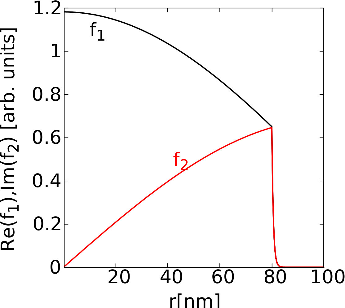 Figure 1
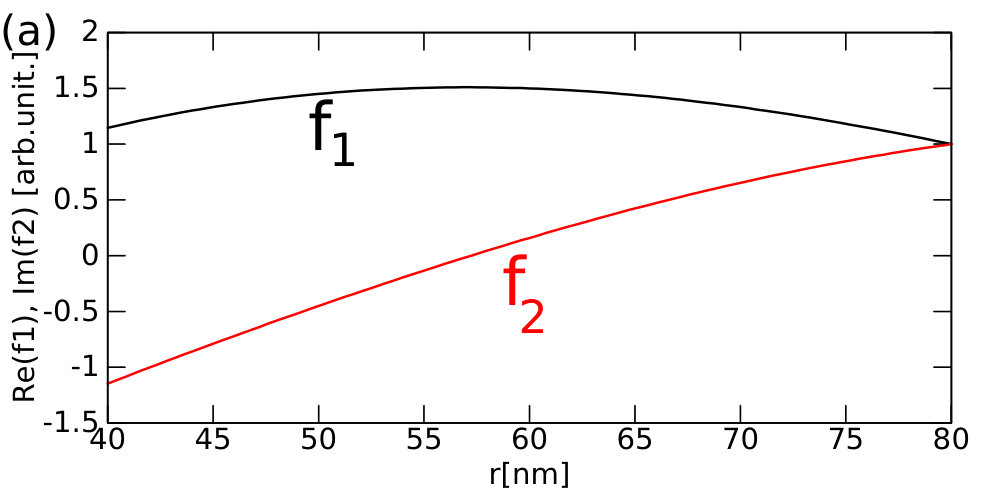 Figure 2
 Figure 3
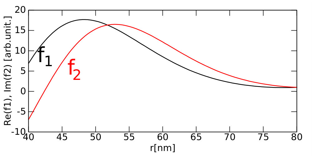 Figure 4
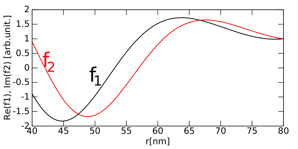 Figure 5
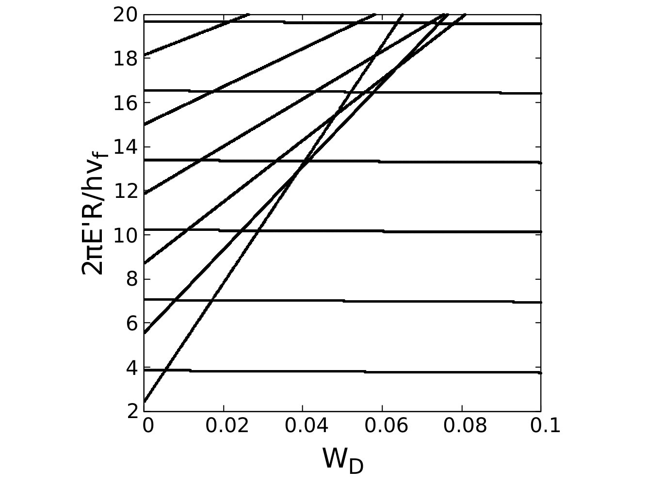 Figure 6
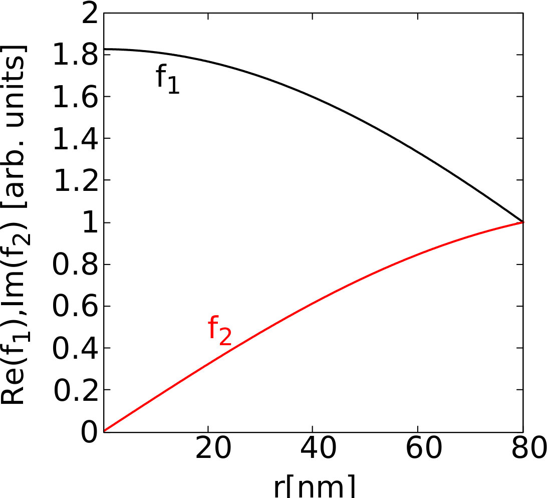 Figure 7
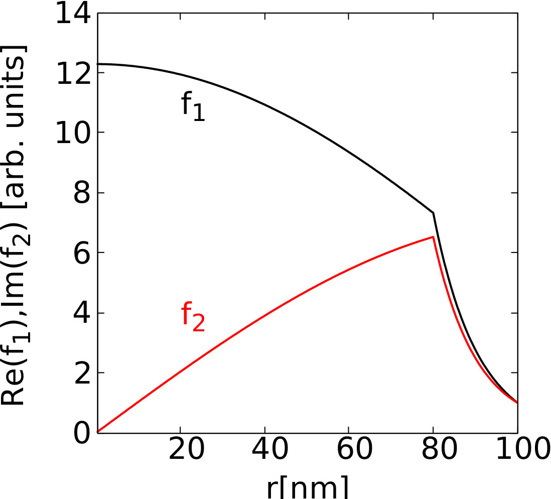 Figure 8
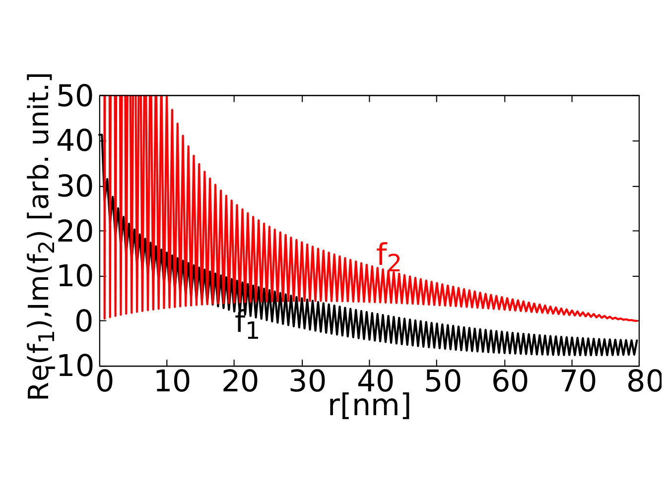 Figure 9
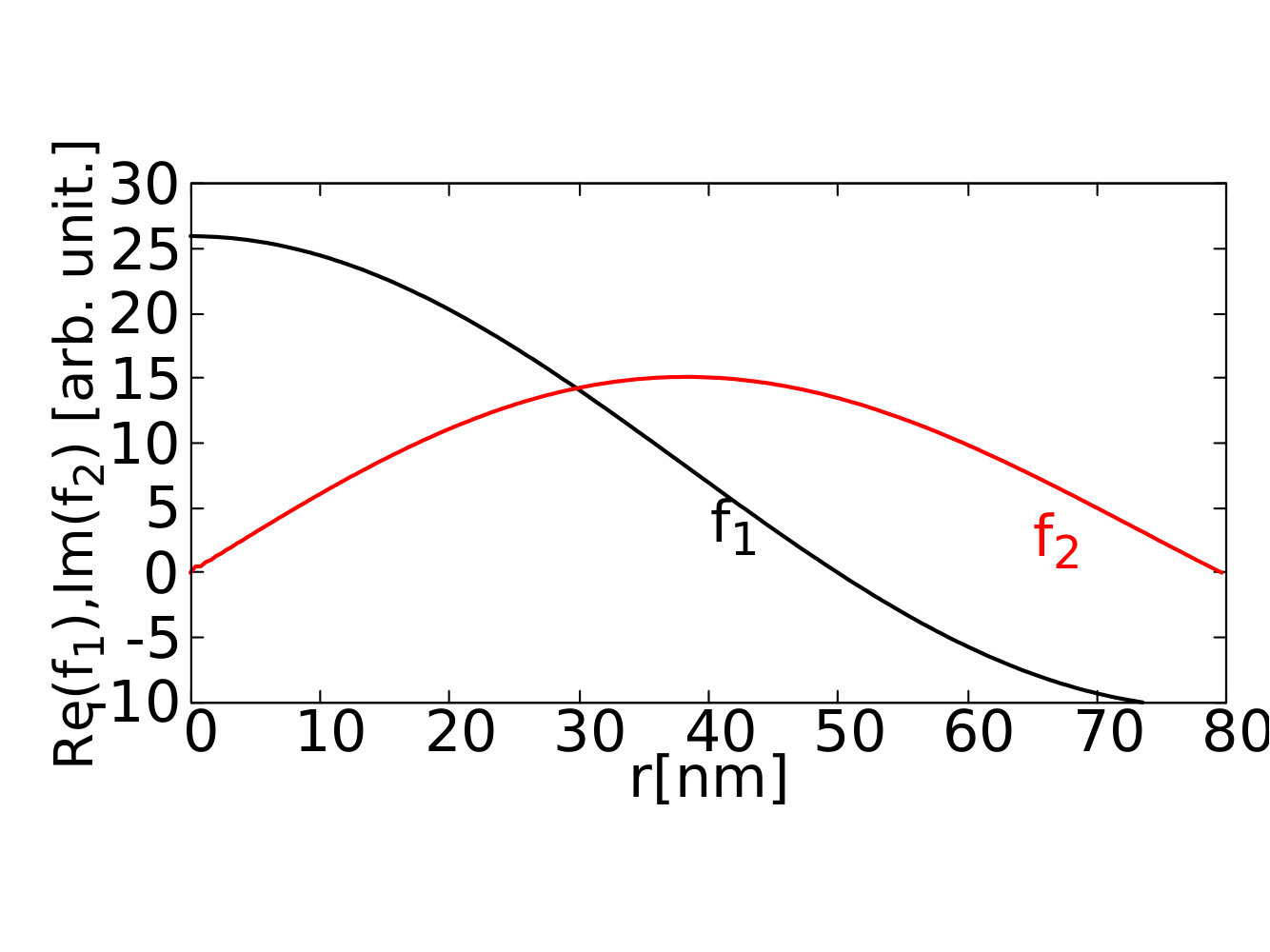 Figure 10
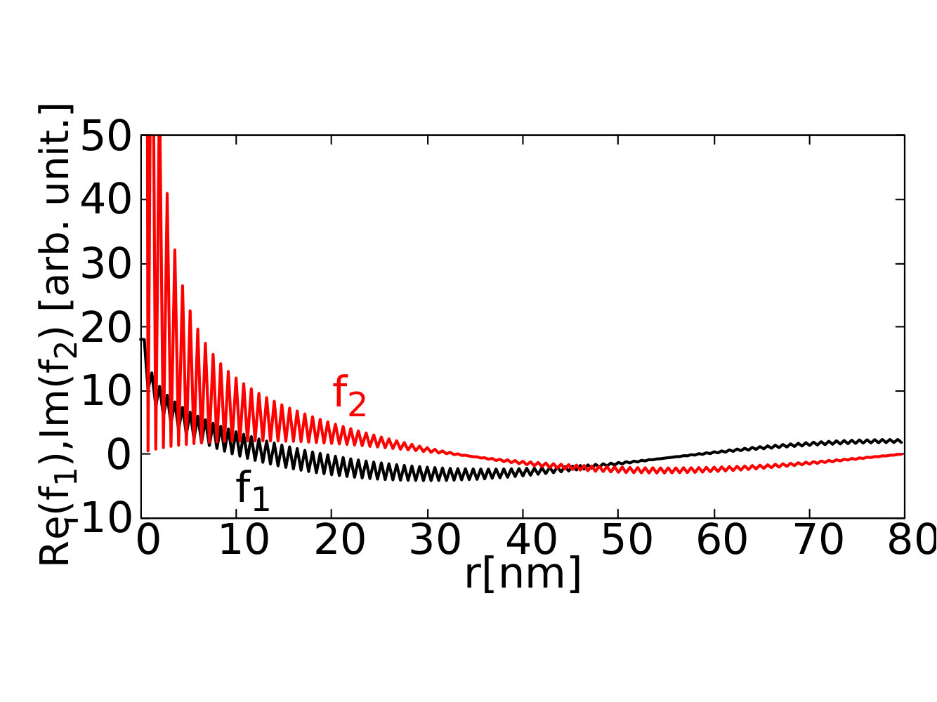 Figure 11
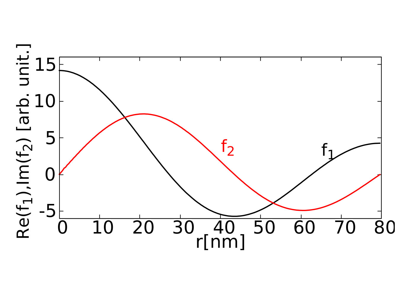 Figure 12
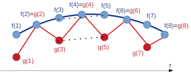 Figure 13
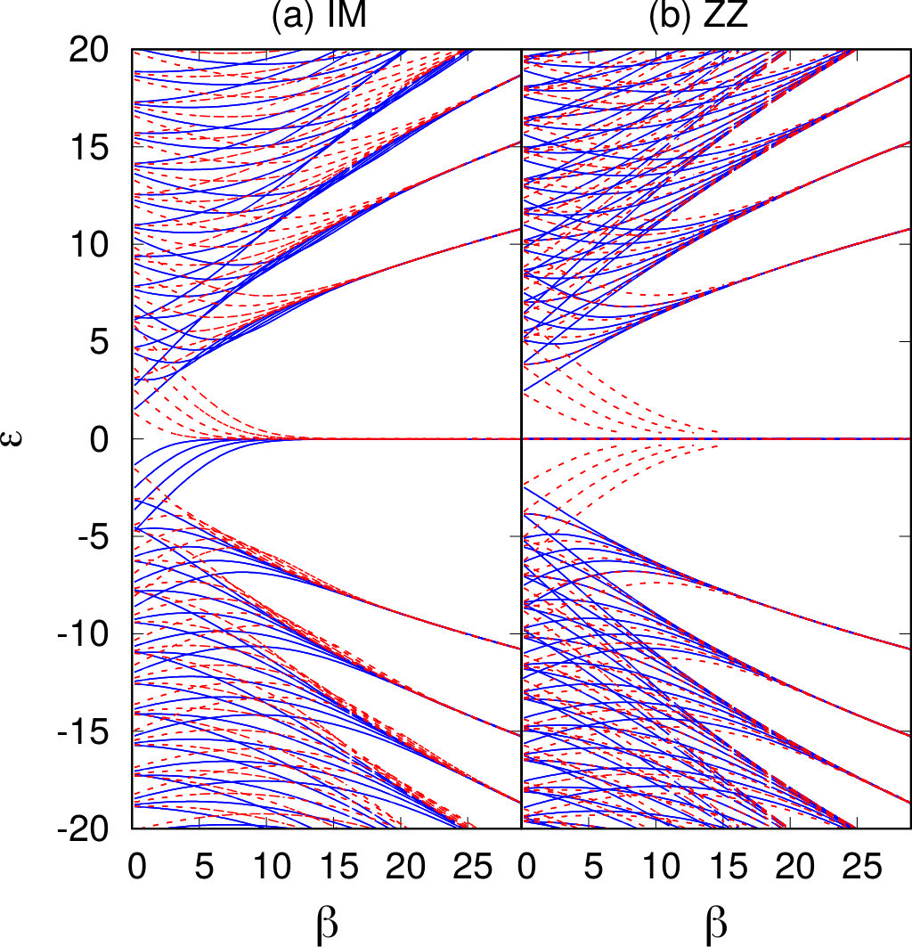 Figure 14
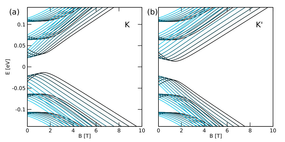 Figure 15
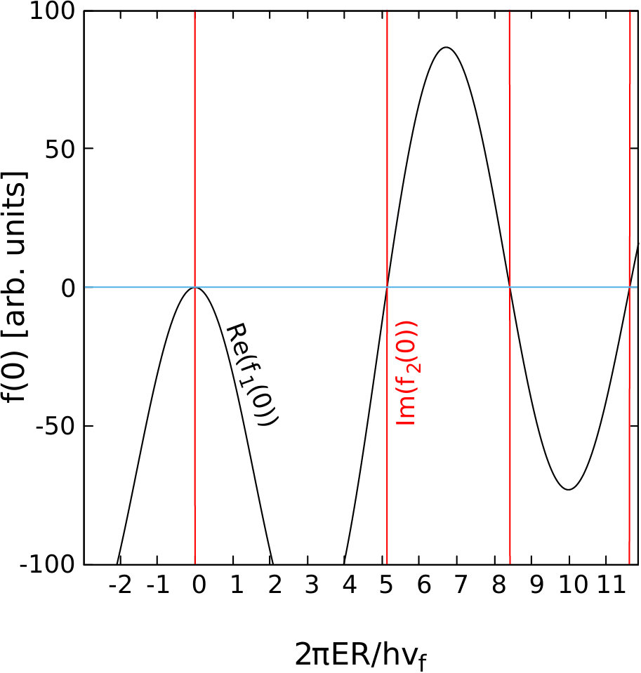 Figure 16
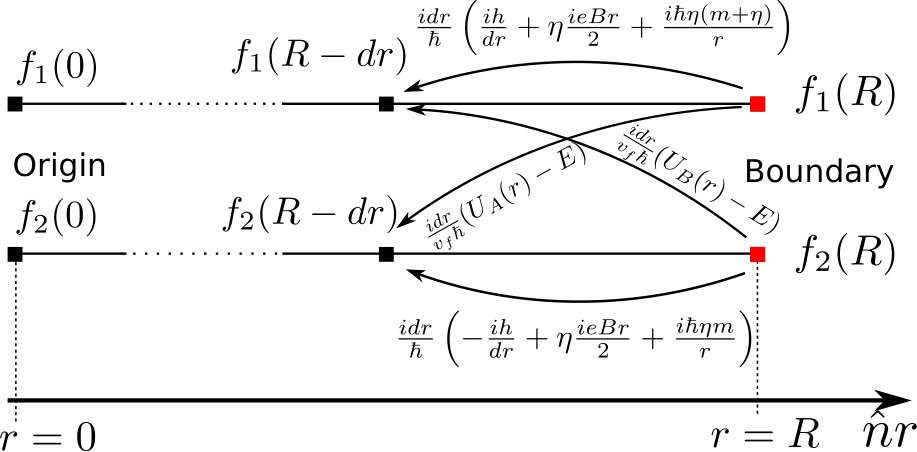 Figure 17
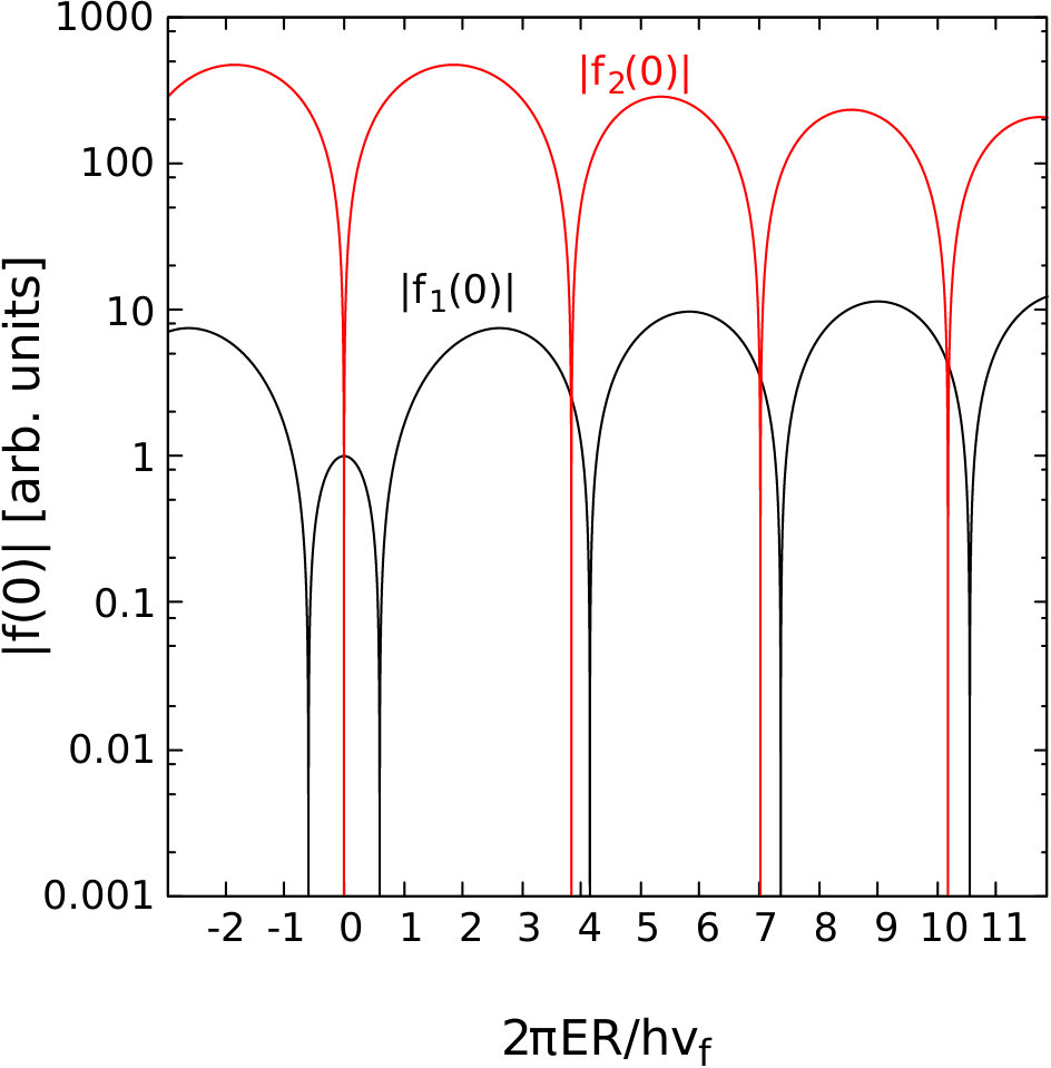 Figure 18
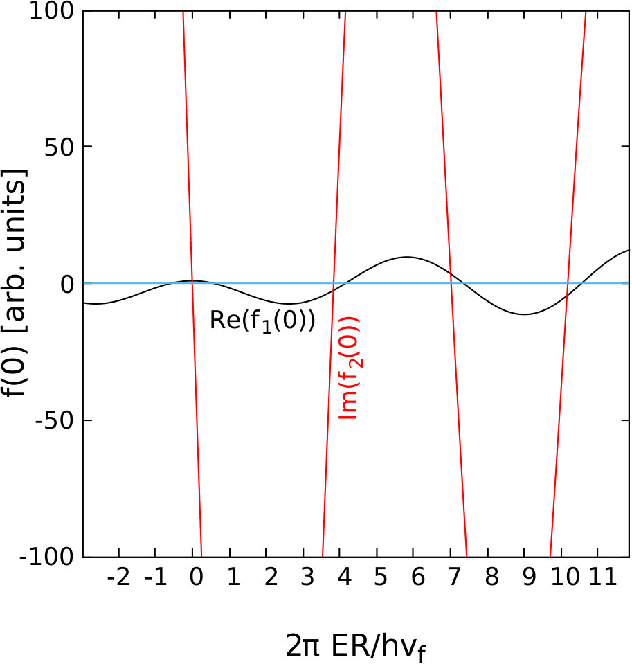 Figure 19
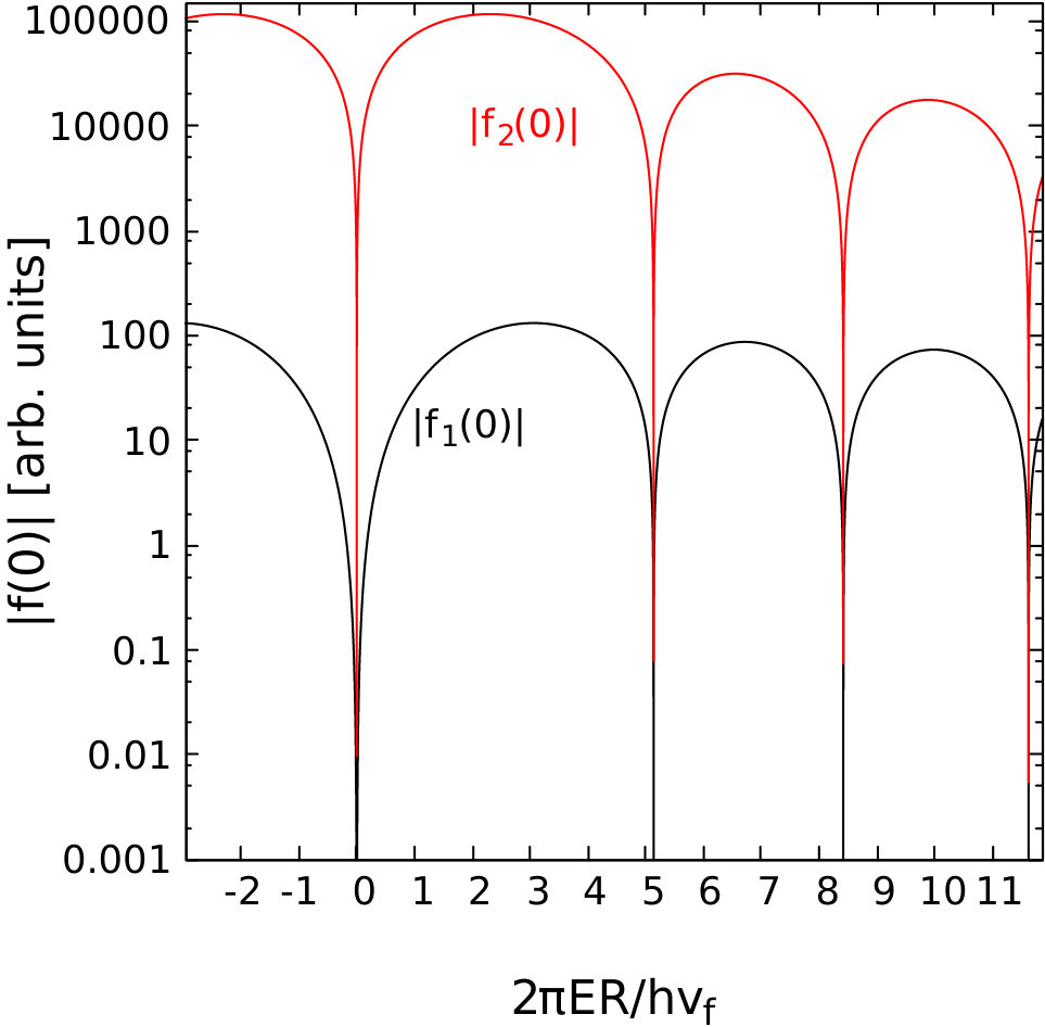 Figure 20
| 3.831706 | 7.015587 | 10.173468 | |
| 2.404825 | 5.520078 | 8.653727 | |
| 3.831706 | 7.015587 | 10.173468 | |
| 5.135622 | 8.417244 | 11.619841 |
| 2.419 | 3.850 | 5.548 | 7.049 | 8.696 | |
| 2.412 | 3.841 | 5.535 | 7.033 | 8.675 | |
| 2.409 | 3.836 | 5.528 | 7.024 | 8.665 |
| 100 | 3.853094 | 7.081613 | 10.304313 |
|---|---|---|---|
| 200 | 3.842100 | 7.046336 | 10.231384 |
| 400 | 3.836828 | 7.030400 | 10.200578 |
| 800 | 3.8342475 | 7.022854 | 10.186564 |
| 1600 | 3.832970 | 7.019184 | 10.179904 |
| 3200 | 3.832339 | 7.017377 | 10.176656 |
| 6400 | 3.832023 | 7.016478 | 10.175054 |
| exact | 3.831706 | 7.015587 | 10.173468 |
| 100 | 0.021388 | 0.066026 | 0.130845 |
| 200 | 0.010394 | 0.030749 | 0.057916 |
| 400 | 0.005122 | 0.014813 | 0.027110 |
| 800 | 0.002541 | 0.007267 | 0.013096 |
| 1600 | 0.001264 | 0.003597 | 0.006436 |
| 3200 | 0.000633 | 0.00179 | 0.003188 |
| 6400 | 0.000317 | 0.000891 | 0.001586 |
Peer Reviews
No public reviews on file for this paper yet. If you reviewed it on a platform where reviews are public (OpenReview, ICLR, NeurIPS, ICML), you can paste yours below so the community can read it here.
Videos
No videos yet. Explain this paper in a talk, walkthrough, or lecture? Add one.
Finite difference method for Dirac electrons in circular quantum dots
Bartłomiej Szafran
Alina Mreńca-Kolasińska
Dariusz Żebrowski
AGH University of Science and Technology, Faculty of Physics and Applied Computer Science, al. Mickiewicza 30, 30-059 Kraków
Abstract
A simple and reliable finite difference approach is presented for solution of the Dirac equation eigenproblem for states confined in rotationally symmetric systems. The method sets the boundary condition for the spinor wave function components at the external edge of the system and then sweeps the radial mesh in search for the energies for which the boundary conditions are met inside the flake. The sweep that is performed from the edge of the system towards the origin allows for application of a two-point finite difference quotient of the first derivative, which prevents the fermion doubling problem and the appearance of the spurious solutions with rapid oscillations of the wave functions.
I Introduction
Numerical solutions of the Dirac equation for relativistic particles have been performed since the 1970’s in the context of the problems of nuclear physics and the lattice gauge theories kogut . The interest in computational approaches for the massless Dirac equation (Weyl equation) has been extended to the solid state with the arrival of graphene neto , the two-dimensional material with gapless and linear dispersion relation near the charge neutrality point.
Solution of the discretized version of the Dirac Hamiltonian on a mesh is commonly pested with spurious solutions that are characterized by rapidly oscillating wave functions, large momenta but low expectation values of the energy kogut ; stacey ; bender ; fermdi ; poszl . The spurious solutions are degenerate with the regular ones which results in the so-called fermion doubling problem kogut ; stacey ; tanimura ; bottcher ; wilson ; susskind ; tworzydlo ; spl4 . The problem arises in particular with the central, three-point discretization of the first order spatial derivative in the Dirac Hamiltonian. The central finite difference quotient misses the wave function oscillations that occur with the periodicity of the mesh spacing stacey ; bender ; bottcher ; tworzydlo . The spurious solutions are also observed in the finite element method poszl despite the exact treatment of shape functions derivatives in this approach. The spurious states can be removed with Wilson approach stacey ; tanimura ; wilson ; susskind that introduces artificial terms in the Hamiltonian depending on the square of the electron momentum, which removes the spurious states from the low-energy spectrum. Alternatively, the shift of the finite difference quotients can be applied which allows the lattice derivative to resolve the rapid oscillations of the wave function stacey ; bottcher ; bender ; tworzydlo .
In this paper, we focus on confined solutions of the Dirac type effective Hamiltonians for graphene. The Weyl fermions evade the confinement by the electrostatic potentials with the Klein tunneling phenomenon k1 ; k2 ; k3 . A way to confine the carriers is to either use a finite flake of graphene gru ; zarenia ; flake1 ; flake2 ; flake4 ; flake5 ; mori ; Yamamoto ; Zhang ; Guclu ; Ezawaf ; Potasz1 ; tho or introduce a non-zero mass in the region outside of the dot berry ; nori . The non-zero mass along with a finite energy gap is introduced to the effective Hamiltonian by the influence of lattice-matched substrates sachs . The gap or non-zero mass can be locally introduced to silicene, a graphene-like 2D hexagonal Si crystal with buckled crystal lattice, using electric fields vertical to the surface ni ; Drummond12 .
In this paper we present a very simple and effective finite difference method for determination of the Dirac Hamiltonian eigenstates localized in circular quantum dots, applicable to both the finite flakes and systems with spatially modulated energy gap. The method is based on a two-point backward derivative. Starting from the boundary condition at the external edge of the flake for the two components of the eigenfunctions one can pin the energies for which the boundary conditions in the interior of the flake are fulfilled for both the spinor components. The proposed mesh-sweeping method resolves only the actual solutions and is free of the spurious ones, hence extra terms in the Hamiltonian of a Wilson type or a post-treatment of the eigenstates are not necessary.
The paper is organized as follows. In Section II we present the Hamiltonian. The analytical solution given in Section III is used for the test calculations. In Section IV we illustrate the problem of the spurious solutions, the fermion doubling and the Wilson procedure using a diagonalization of the finite difference Hamiltonian with the central three point lattice derivative. The original method reported in this work is presented in Section V. Examples of applications, including the spatial variation of the energy gap and a graphene quantum ring are presented in Section VI. The summary is given in Section VII.
II Hamiltonian
The effective low-energy Dirac Hamiltonian for electrons in graphene or silicene can be separated into two operators each associated with one of the non-equivalent valleys of the Brillouin zone, or . These valleys will be referred to by the index and , respectively. The Hamiltonian for the valley index takes the form neto
[TABLE]
where is the Fermi velocity, , and is the vector potential. This Hamiltonian acts on a wave function of form \Psi({\bf r})=\left(\begin{array}[]{c}\Psi_{1}({\bf r})\\ \Psi_{2}({\bf r})\end{array}\right), whose components correspond to the A and B graphene sublattices neto , respectively. In Eq. (1), and stand for potentials at the two sublattices. The potentials can be made unequal due to the substrate of e.g. a hexagonal boron nitride sachs . Vertical electric field applied to a graphene-like 2D hexagonal crystal with the buckled crystal lattice, e.g. the silicene also introduces unequal and values, that introduces the energy gap to the dispersion relation ni ; Drummond12 .
Hamiltonian for a circular flake of graphene in the vertical magnetic field and symmetric gauge commutes with generalized angular momentum operator , where is the z-component of the orbital angular momentum. For the polar coordinates: and , the operator is and is the Pauli matrix in the sublattice space. Therefore, the stationary states can be labeled with magnetic quantum number and have form
[TABLE]
The radial functions and of Eq. (2) are solutions to the system of eigenequations
[TABLE]
III Analytical solution
An analytical solution gru ; tho to Eq. (3) without the external fields will be used for the test calculations. For and , Eq. (3) reads
[TABLE]
For one can eliminate from (5) and plug it into (4) to obtain
[TABLE]
which upon introduction of a dimensionless radial coordinate , produces the Bessel equation
[TABLE]
where, up to a normalization constant , and is the th Bessel function of the first kind. Using identities bee , , one finds . For the test calculations we take a finite flake of radius and apply a so-called zigzag boundary condition gru . For the flake that is terminated by the sublattice, the second component of the wave function – that describes the sublattice, needs to vanish at , hence . This condition defines the spectrum of the states confined within the flake, where numbers the eigenvalues for fixed . For the conduction band states we use positive values of . From the boundary condition we find the non-zero energy eigenvalue
[TABLE]
where is the th zero of Bessel function bee – see Table 1.
IV Diagonalization of the finite difference problem
For illustration of the problem of spurious solutions, we solve Eqs. (4,5) in a finite difference approach using diagonalization of the resulting algebraic equations. For that purpose we need a boundary condition at the origin. The radial functions , , near behave as and , respectively. A natural Dirichlet condition at independent of the orbital angular momentum can be obtained by substitution for . Since is finite at , needs to vanish at the origin independent of . The system of eigenequations for functions then reads
[TABLE]
The boundary conditions are then at the origin and the zigzag boundary at the edge , . We use points on the radial mesh, including the origin where the boundary conditions are applied, and the discretization step . For discretization we use the difference quotient with the exception of the last point on the mesh for , where a two point formula is used . The resulting algebraic eigenequation is described by a non-symmetric matrix and is solved with the ARPACK library (procedure ZGEEV).
For the numerical calculations we use , for the silicene tight-binding hopping energy of eV and the nearest neighbour distance of nm. For the radius of the flake we take nm. The positive eigenenergies are listed in Table 2 for , and and a varied number of points on the spatial mesh. In Table 2 we number the eigenstates by – the number that counts also the spurious states – to distinguish from the actual quantum number used in Table 1 and below. For and one would expect to obtain the values given by and – see Table 1. The other values are the energies of the spurious states. In fact, the energies of spurious solutions obtained for correspond to the regular eigenstates but for a different . In particular, the energies for odd of Table 2 that were calculated with correspond to the exact energies for – see Table 1. With the spurious solutions the degeneracy of energy levels is artificially increased by a factor of two, which produces the fermion doubling problem kogut ; stacey ; tanimura ; bottcher ; wilson ; susskind ; tworzydlo ; spl4 .
The wave functions for from 1 to are displayed in Fig. 1. With the applied boundary conditions is real and is imaginary. The spurious states [Fig. 1(a,c)] correspond to the real part of and imaginary part of that rapidly oscillate between the nearest-neighbor mesh points. The solution given by Fig. 1(b,d) corresponds to the analytical eigenstates.
In the spurious solutions is large due to the rapid wave function oscillations (see Fig. 1(a,c)). Using this fact one can numerically remove the spurious states from the low-energy part of the spectrum. The procedure stacey ; tanimura ; wilson ; susskind involves an extra artificial energy operator of form
[TABLE]
where is a dimensionless Wilson parameter. Figure 2 shows the energies of the , states (same as in Fig. 1 and Table 2), where is introduced by the first order perturbation . The states identified as spurious in the context of Table 2 and Fig. 1 are indeed removed from the low-energy spectrum, while the actual solutions are only weekly affected by the Wilson term.
V The mesh sweeping method
We are ready to introduce the method which is the purpose of this work. The method provides the solution of the Dirac equation on a finite difference mesh and is free of the spurious states, so no discrimination of the rapidly oscillating states is necessary. The general system of equations given by Eq. (3) is transformed to a form that allows for sweeping the mesh from the edge of the flake to its center. For this purpose the radial derivative is replaced by a two-point finite difference quotient . The sweeping finite difference scheme is
[TABLE]
The schematics of the calculations given in Fig. 3. The procedure starts at the edge of the flake , where the boundary conditions are applied. For the zigzag boundary condition we set and . The eigenfunctions can be normalized after the entire procedure. With the starting values of and at one can proceed to the center of the flake using Eqs. (11) and (12). At the origin and need to vanish when and , respectively. That, in turn is realized only for discrete values of the energy. For , the values of the components of the wave function for are given in Fig. 4 for (left column) and (right column). For the component needs to vanish at the origin, since the angular momentum quantum number corresponding to the second component is nonzero, . The position of the energy eigenvalues can be found as the minima of the absolute values of the [Fig. 4(a)] or equivalently, by zeroes of the imaginary part of [see Fig. 4(c)] as a function of the energy. The minima [Fig. 4(a)] and the zeroes [Fig. 4(c)] correspond to the actual eigenvalues and the spurious solutions are missing [cf. Tables 1 and 2]. For both and components need to vanish at the origin, and indeed no shift of the minima of Fig. 4(b) or zeroes of Fig. 4(d) is observed on the energy scale. Besides the solutions of the Bessel form, the results of Fig. 4 indicate the presence of the zero-energy levels that are supported by the zigzag edge gru .
The success of the sweeping approach is due to the two-point derivative that does not allow for saw-like oscillations of the wave function. To explain this let us look at Fig. 5 where two functions: a smooth one and a rapidly oscillating one are plotted on a radial mesh. For even indexes functions and are equal and for odd indexes a shift between the solutions is present. From the point of view of the central quotient of the first derivative both the solutions are identical; in each mesh point the same value of the quotient are obtained, and there is no relation between the odd and even indexes on the mesh points, which allows for the spurious states to appear in the low-energy part of the spectrum. The Wilson term given by Eq. (10) introduces the second derivative with the quotient that links the odd and even points and removes the rapidly oscillating states from the low-energy spectrum. The sweeping method that uses the backward quotient and passes through each mesh point consecutively introduces the link between the even and odd mesh points. The two-point formula for the smooth and rapidly oscillating solutions produce very different values of the quotient.
Tabel 3 shows that the convergence of the results of the present method to the exact solution is linear as a function of (or ). Although the convergence is slow, the numerical cost of the calculation increases only linearily with , and the method needs to keep track of only four complex numbers for the wave function components at adjacent mesh points, so one can approach the exact solution arbitrarily close at a negligible numerical cost.
VI Examples of applications
The approach is suitable for any radial problems involving the effective Hamiltonian that stems from the Dirac equation for a given valley. This section provides examples of applications.
VI.1 Limit of infinite-mass confinement
In the precedent section the zigzag-boundary conditions were used that result from a specific termination of the crystal lattice. The confinement of the particle described by the Dirac Hamiltonian can be induced provided by e.g. a spatial dependence of the energy gap nori of equivalently by an external potential due to e.g. a substrate sachs .
For an energy gap is opened in the dispersion relation near the Dirac points and the carriers acquire finite masses. For and that diverge to and when , respectively, the mass in the outside of the confinement is infinite and the wave functions of finite energies vanish at berry ; huang ; nipre . The boundary condition for this type of confinement is derived from vanishing current at the edge berry of the confinement area. The probability density current that is derived from the Hamiltonian berry is . For the infinite mass at the outside of the dot, the orthogonal component of the current must vanish , which implies .
With Eq. (2) this condition is translated for the radial functions as To fulfill this condition we set at the end of the flake , and , for which one gets , which is fulfilled for both the valleys .
Let us look at the appearance of the wave functions confinement by the mass boundary. We consider a spatial dependence of the energy gap as introduced by finite potentials. Figure 6 shows the real part of and the imaginary part of for and . At the end of the flake the infinite mass boundary condition is applied. The components and are – as for the zigzag boundary – purely real and purely imaginary, respectively. Moreover, the infinite-mass boundary condition implies . The results of Fig. 6(a) were obtained for a flake of radius nm in the absence of the external potentials. In Fig. 6(b,c) we extended the flake to nm but introduced the energy gap beyond nm with . In Fig. 6(a), eV and eV in Fig. 6(c). We can see that for larger the functions penetrate only weakly into the gapped region for nm, and the values and become equal at , where the gap is introduced. In this way the infinite boundary condition is found in the limit of large at .
VI.2 The quantum ring spectra
The method with a slight modification can be applied to a problem of a graphene quantum ring tho . From the flake of the radius of nm we remove the central disk of a radius of nm. The infinite mass boundary condition in the inner edge of the flake reads . We start from the external edge as in the precedent subsection. The sweep at the finite difference mesh stops ar . From the inner boundary condition we construct a function and we look for its zeroes as a function of the energy.
The wave functions for the valley () found in this way are displayed in Fig. 7 for (a,b) and (c,d). The energy spectra for are given in Fig. 8 for . In the lowest energy states of the conduction and the valence bands one observes the characteristic angular momentum transitions with the Aharonov-Bohm periodicity of T pers , that corresponds to a flux quantum threading a ring of an effective radius nm – close to the central radius of the ring .
VI.3 Comparison with analytical results in the external magnetic field
In the absence of the external potential , or for a massless particle, analytical results were obtained for the Weyl equation in the external magnetic field in Ref. gru for both zigzag and infinite mass boundary conditions. We adopted the graphene parameters of this work gru eV, the lattice constant nm and the radius of the dot nm. The results for the 500 mesh points are displayed in Fig. 9 with a perfect agreement with Fig. 1 of Ref. gru .
VII Summary
We have presented the finite difference method, applicable to Dirac carriers in circular confinement, that sweeps the mesh from the external edge of the system, where the boundary conditions are defined, to the center. The energies of the confined states are pinned by the internal boundary conditions. The method is simple, free of spurious solutions and the fermion doubling problem. Applications to circular flakes, quantum rings, and the energy gap modulated in space were presented.
Acknowledgments
This work was supported by the National Science Centre (NCN) according to decision DEC-2016/23/B/ST3/00821.
The reference list from the paper itself. Each links out to its DOI / PubMed record.
- 1(1) J.P. Kogut, Rev. Mod. Phys. 55 , 775 (1983).
- 2(2) A. H. Castro Neto, F. Guinea, N. M. R. Peres, K. S. Novoselov, and A. K. Geim, Rev. Mod. Phys. 81 , 109 (2009).
- 3(3) C.M. Bender, K.A. Milton, and D.H. Sharp, Phys. Rev. Lett. 51 , 1815 (1983).
- 4(4) J. C. Wells, V. E. Oberacker, A. S. Umar, C. Bottcher, M. R. Strayer, J.-S. Wu, and G. Plunien Phys. Rev. A 45 , 6296 (1992).
- 5(5) W. Poeschl, D. Vretenar, and P. Ring, Comp. Phys. Comm. 99 (1996) 128.
- 6(6) R. Stacey, Phys. Rev. D 26 468 (1982).
- 7(7) C. Bottcher, M. R. Strayer, A. S. Umar, and P.-G. Reinhard Phys. Rev. A 40 4182 (1989).
- 8(8) J. Tworzydło, C.W. Groth, and C.W.J. Beenakker, Phys. Rev. B 78 (2008) 235438.