Imaging point sources in heterogeneous environments
Kui Ren, Yimin Zhong

TL;DR
This paper studies how uncertainties in the environment's refractive index affect the accuracy of imaging point sources using boundary or far-field measurements, providing stability results and numerical validation.
Contribution
It extends existing imaging theories by analyzing the impact of environment uncertainty on source reconstruction stability in heterogeneous media.
Findings
Reconstruction stability is maintained under measurement errors.
Smooth variations in the environment have limited impact on imaging accuracy.
Numerical simulations confirm theoretical stability results.
Abstract
Imaging point sources in heterogeneous environments from boundary or far-field measurements has been extensively studied in the past. In most existing results, the environment, represented by the refractive index function in the model equation, is assumed known in the imaging process. In this work, we investigate the impact of environment uncertainty on the reconstruction of point sources inside it. Following the techniques developed by El Badia and El Hajj (C. R. Acad. Sci. Paris, Ser. I, 350 (2012), 1031-1035), we derive stability of reconstructing point sources in heterogeneous media with respect to measurement error as well as smooth changes in the environment, that is, the refractive index. Numerical simulations with synthetic data are presented to further explore the derived stability properties.
Click any figure to enlarge with its caption.
 Figure 1
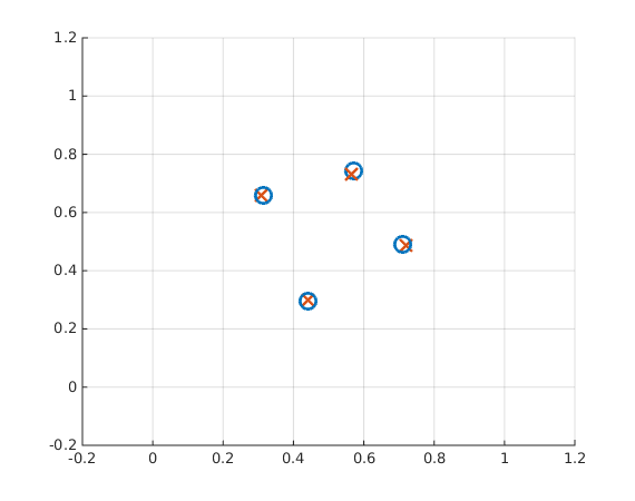 Figure 2
 Figure 3
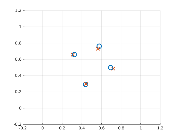 Figure 4
 Figure 5
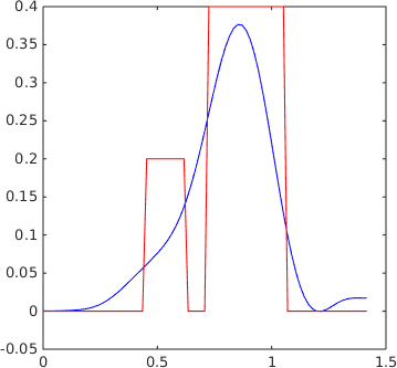 Figure 6
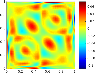 Figure 7
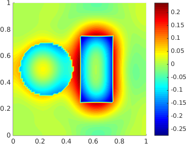 Figure 8
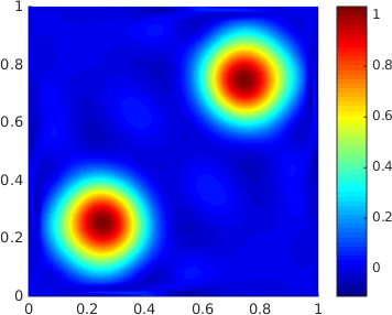 Figure 9
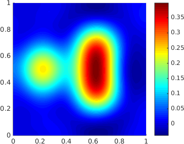 Figure 10
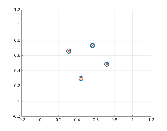 Figure 11
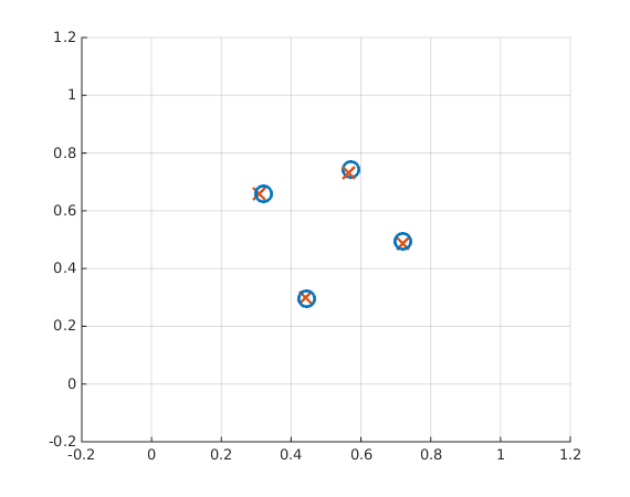 Figure 12
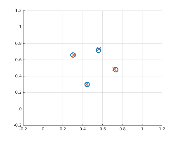 Figure 13
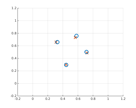 Figure 14
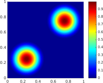 Figure 15
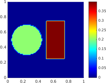 Figure 16
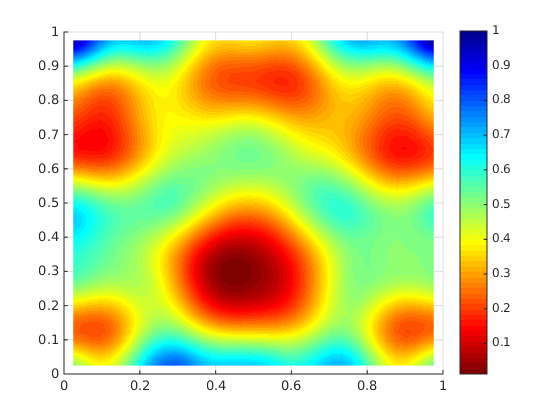 Figure 17
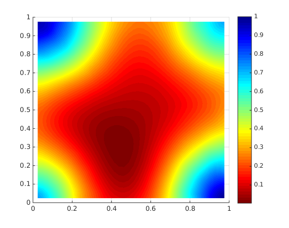 Figure 18
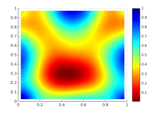 Figure 19
| \@tabular@row@before@xcolor \@xcolor@tabular@before Experiment | True value | Reconstructions with noisy data | |
| \@tabular@row@before@xcolor \@xcolor@row@after | 1% noise | 5% noise | |
| \@tabular@row@before@xcolor \@xcolor@row@after1: medium (33) | (0.89,0.73,0.71,0.52) | (0.91,0.73,0.68,0.54) | (0.92,0.65,0.76,0.46) |
| \@tabular@row@before@xcolor \@xcolor@row@after1: medium (34) | (0.89,0.73,0.71,0.52) | (0.88,0.72,0.71,0.52) | (0.88,0.72,0.69,0.54) |
| \@tabular@row@before@xcolor \@xcolor@row@after2 | (0.89,0.73,0.71,0.52) | (0.91,0.76,0.65,0.58) | (0.87,0.83,0.56,0.64) |
| \@tabular@row@before@xcolor \@xcolor@row@after3 | (0.89,0.73,0.71,0.52) | (0.90,0.81,0.65,0.56) | (0.89,0.85,0.61,0.60) |
| \@tabular@row@before@xcolor \@xcolor@row@after | |||
\@tabular@row@before@xcolor \@xcolor@row@after
The simulations show that one can indeed reconstruct point sources, both their locations and their intensities, inside heterogeneous media when the media are not unreasonably complex. We want to emphasize here that in our theoretical analysis as well as numerical simulations, both the true sources and the sources to be reconstructed are explicitly assumed to be point sources. In other words, we explicitly search for the locations and strengths of the point sources, instead of reconstructing spatially distributed sources hoping that the result will give us point sources. In general, we observe from our extensive numerical simulations that when the refractive index is exactly known, the reconstructions are quite stable when the number of point sources is small. However, the reconstructions become too sensitive to algorithmic parameters when the number of point sources gets large.
We also want to emphasize that it is important to impose the constraints on the separability of the point sources in the numerical simulations. In other words, we have to explicitly ensure that the point sources to be reconstructed are far away from each other. Even in this case, the reconstructions are sensitive to the initial guess of the locations of the point sources. The objective function that we minimize to reconstruct the point sources can not differentiate between the true point sources and the equivalent class of re-labeled point sources. Therefore, the minimization algorithm could be easily fooled to jump between different intermediate configurations if the point sources are not well-separated. To further illustrate on this issue, we plot in Figure 3 the (normalized) objective functional defined in (28) as a function of the location of a single point source (the intensity of the source being assumed known). The true point source is located at . While it is clear from the plot that the objective function is convex with respect to the location of the point source when , this is not true anymore when and . In the case of , two local minmizers emerge at . More local minimizers emerge when . These plots show that even in the case of a single point source, when the initial guess is far from the true position, the minimization algorithm could return wrong reconstructions. We can not visualize this phenomenon in the case of more than one point source. However, one can easily imagine that the situation would be far worse in that scenario.
Experiment 2 [Recovery in an Unknown Environment].In the second set of simulations, we reconstruct point sources in medium (33) assuming that both the medium and the point sources are not known. The reconstructions of the medium and the locations of the sources are shown in Figure 3 and the reconstructed intensities of the point sources are summarized in the third row of Table 3. |
|||
\@tabular@row@before@xcolor \@xcolor@row@afterExperiment 3 [Recovery in an Unknown Environment]. |
|||
Peer Reviews
No public reviews on file for this paper yet. If you reviewed it on a platform where reviews are public (OpenReview, ICLR, NeurIPS, ICML), you can paste yours below so the community can read it here.
Videos
No videos yet. Explain this paper in a talk, walkthrough, or lecture? Add one.
{psinputs}
Imaging point sources in heterogeneous environments
Kui Ren
Department of Applied Physics and Applied Mathematics, Columbia University, New York, NY 10027; [email protected]
Yimin Zhong
Department of Mathematics, University of California, Irvine, CA 92697-3875; [email protected]
Abstract
Imaging point sources in heterogeneous environments from boundary or far-field measurements has been extensively studied in the past. In most existing results, the environment, represented by the refractive index function in the model equation, is assumed known in the imaging process. In this work, we investigate the impact of environment uncertainty on the reconstruction of point sources inside it. Following the techniques developed by El Badia and El Hajj (C. R. Acad. Sci. Paris, Ser. I, 350 (2012), 1031-1035), we derive stability of reconstructing point sources in heterogeneous media with respect to measurement error as well as smooth changes in the environment, that is, the refractive index. Numerical simulations with synthetic data are presented to further explore the derived stability properties.
Key words. Inverse source problems, Helmholtz equation, point sources, stability estimates, numerical reconstructions, uncertainty characterization, inverse problems
AMS subject classifications 2010. 15A29, 35R30, 49N45, 65N21, 78A46.
1 Introduction
Recovering radiative sources inside heterogeneous media from boundary or far-field measurements has applications in many branches of science and technology [AmBaFl-SIAM02, Baltes-Book78, BaLiTr-JDE10, BaBeBeLe-IP05, CaEw-IPBVP75, Chin-ACM10, ElVa-IP09, GaOsTa-JIIPP13, HoCl-MB97, Ikehata-IP99, ImYa-IP98, IsLu-IPI18, JiLiYa-JDE17, Larsen-JQSRT73, MaTs-IP13, Nicaise-SIAM00, PuYa-IP96, Sezginer-IP87, Siewart-JQSRT93, Yamamoto-IP95]. Extensive mathematical and computational studies of such inverse source problems have been performed in the past decades; see, for instance, [AnBuEr-Book97, Isakov-Book90, Isakov-Book06] and references therein for recent reviews on the subject.
In this work, we are interested in a source recovery problem where the source to be reconstructed is the superposition of point sources [BaBeBeLe-IP05, CaEw-IPBVP75, ElBadia-IP05, ElHa-JIIPP02, ElEl-CRASP12, ElNa-IP11, FaHaEs-IPI13, GaZhCoWa-BOE10, KaLe-IP04, KoYa-IP02, LiTa-CiCP09, MaTs-IP13, OhInOh-IP11, Vessella-IP92]. Unlike general source functions, point sources are efficiently characterized by their locations and strengths, a fact that significantly reduces the dimension of the parameter space of the inverse problems. This dimension reduction often enables one to obtain uniqueness in the inverse problem with minimum amount of observed data and provides the possibility of utilizing efficient reconstruction algorithms, for instance these based on compressive sensing [ChMoPa-IP12, FaStYa-SIAM10], in the source recovery process.
To formulate our problem, let () be a simply connected domain with boundary . Let be the solution to the following boundary value problem to the Helmholtz equation:
[TABLE]
where the real-valued function is the refractive index, and are internal and boundary source terms respectively. We assume that has a compact support in , that is, , and that , . We assume that [math] is not an eigenvalue of the operator with homogeneous Dirichlet boundary condition such that the problem (1) admits a unique solution for given source functions and .
We assume that the internal source function is a superposition of point sources located at with strengths , that is,
[TABLE]
The strengths are all assumed to be real-valued so that there is no physical absorption occurring at the point sources.
The Helmholtz equation (1) can be viewed as a simplified frequency-domain model for either electromagnetic or ultrasound wave propagation, depending on the value of the parameters, mainly the wavenumber , in the equation. The mathematical derivations in the rest of the paper implicitly assume that the wavenumber is real-valued and . We believe, however, the same types of calculations can be carried out for the zero-frequency case () as those studied in [BaBeBeLe-IP05, ElBadia-IP05] or in [WaLiJi-MP05] with an extra absorption term.
Let us also mention that since linearizing inverse coefficient problems often results in inverse source problems, the point source reconstruction problem we study in this paper is closely related to the problem of reconstructing small volume inclusions in background media [AmKa-IP03, AmMoVo-ESAIM03] and the problem of imaging small scatterers in complex media [BoPaTs-IP03, BoPaTs-IP05, ChMoPa-IP16, DeMaGr-JASA05]. The main difference is that in our derivation below, we can utilize explicitly the fact that point sources are singular. The secondary sources created by small scatterers or inclusions, however, do not carry the same level of singularity of the point sources.
We are interested in the problem of reconstructing the point sources, i.e. their locations and strengths, from Cauchy data where the boundary measurement is given as
[TABLE]
being the unit outer normal vector of the domain boundary at .
To our best knowledge, in all the previous work on point source recovery, the environment, that is, the refractive index in our formulation, in which point sources (or point source like localized objects), are to be sought is assumed to be known exactly, with the only exception in [BuLaTaTs-AFR09] where the authors tried to reconstruct point sources in homogeneous media with unknown impenetrable obstacles. In other words, in the environment under which the data are collected is the same as the environment that data are back-propagated to reconstruct the point sources. Moreover, the mathematical works where stability of source reconstructions are derived with respect to noise in measured data are all done under the assumption that the environment is homogeneous (so that one could have access to the explicit form of the associated Green’s function).
In the rest of the paper, we prove a stability result, following the techniques developed by El Badia and El Hajj (C. R. Acad. Sci. Paris, Ser. I, 350 (2012), 1031-1035) [ElEl-CRASP12], on the recovering of point sources in smooth inhomogeneous environment, that is, when the refractive index varies smoothly in space. We also prove the stability of point source reconstruction with respect to smooth changes in the environment: if we perform reconstructions in a medium that is only slightly, in appropriate sense, different than the medium from which we collected the data, then the reconstructions are only slightly different from the reconstructions in the exact medium that generated the data.
2 Main results
We now present the main result of this short paper: (i) the stability of reconstructing point sources in an heterogeneous medium; and (ii) the stability of the reconstructions with respect to smooth changes of the medium.
2.1 Stability in heterogeneous media
We first consider the case where the underlying medium is known but heterogeneous, that is, we have a known but spatially varying refractive index . Under this circumstance, we can uniquely reconstruct the source from a single pair of Cauchy data with a given Hölder type of stability. This is a generalization of the stability results of El Badia and El Hajj established in [ElEl-CRASP12, ElNa-IP11].
We make the following general assumptions on the setup of the problem.
(A). The domain has a boundary . The refractive index is real-valued and smooth, with support . The point sources are well separated in the sense that for some . The point sources are sufficiently far away from the boundary of the domain such that , , for some . The strengths of the point sources satisfy , , for some and . The illumination boundary source is the restriction of a function to .
It will be clear that the smoothness assumptions on the refractive index and the boundary source are not completely necessary. In fact, being is sufficient for all the results to hold. It should also be noted that the assumptions on the point sources imply that whenever , a fact that is implicitly used later when we study uniqueness of reconstructions.
Lemma 2.1**.**
Let
[TABLE]
be two sets of point sources satisfying the assumptions in (A), () the corresponding solutions to the Helmholtz equation (1). Then implies that and
[TABLE]
for some permutation .
Proof.
This result follows from the unique continuation principle for Cauchy problems of elliptic equations. Let be the disk centered at with radius small enough such that . We define and verify that solves
[TABLE]
Since , we then conclude from the unique continuation principle [Isakov-Book06, Theorem 3.3.1] that , with any . If we take , this implies that except at the locations . Therefore must be a finite linear combination of point sources and their derivatives. This is impossible. Therefore up to a possible permutation , that is, renumbering of the point sources. ∎
We now study the stability of the reconstruction. Following [ElEl-CRASP12, ElNa-IP11], we look at the stability issue for an algebraic reconstruction technique that is based on the projection of the point sources into planes in . Due to the fact that the medium is heterogeneous, we need to find good ways to do the projection. In the next two lemmas, we introduce our method of projection onto surfaces determined by the solutions of the Helmholtz equation (which are controlled by the medium).
Lemma 2.2**.**
Under the assumptions in (A) on the refractive index and , there exists a complex-valued function and a constant such that solves
[TABLE]
, , and
[TABLE]
Proof.
With the regularity of assumed in (A), we can take as the well-known complex geometrical optics (CGO) solution to (6); see for instance [NaUhWa-IP13]. More precisely, let with and given vectors such that and (i.e. ). It is shown in [NaUhWa-IP13] that (6) has a solution of the form
[TABLE]
when is sufficiently large. Then by the Sobolev embedding theorem [AdFo-Book03], . If we choose large such that , then we will have for all and . Therefore we can find a constant such that
[TABLE]
This completes the proof. ∎
Definition 2.3**.**
The function introduced in Lemma 2.2 defines a local frame on , where , and forms an unitary matrix, which also determines a local coordinate change , denoted by , from the Cartesian coordinate to the local frame. We define a projection as:
[TABLE]
This projection defines a pseudo distance function and the diameter of under the projection is denoted by .
The project we defined here is clearly not unique in the sense that one can rotate the coordinates to use or to replace and . Moreover, since can be chosen differently using the complex vector (which controls the boundary condition needed), we can construct the that we need by selection a specific vector.
The projection we just introduced allows us to construct the following test functions.
Lemma 2.4**.**
Let be arbitrary distinct points. Then under assumption (A), there exists a function solving
[TABLE]
such that
[TABLE]
Proof.
We construct the function as follows:
[TABLE]
Then clearly , . It is straightforward to verify that and , which allow us to check that solves (8). ∎
We are now ready to prove the stability of the reconstruction. Our reconstruction scheme follows a two-step process. In the first step, the locations of the point sources are probed by a projection method. In the second step, we use the reconstructed locations to reconstruct the strengths of the point sources .
Theorem 2.5**.**
Let and be two sources of the form (4) with that are reconstructed from the Cauchy data and respectively. Let be the projection in Definition 2.3. Let and assume that . Then, under the assumptions in (A), there exists a permutation acting on and a constant depending on , , , and , such that
[TABLE]
where is the surface measure of . Assume further that , and let , then there exists constants and , again depending on , , , and , such that
[TABLE]
Proof.
Let be the solution to the Helmholtz equation (1) with source . We define . Then solves the Helmholtz equation (1) with boundary data . Let be an integer. From Lemma 2.4, we find a function, being defined in Lemma 2.2,
[TABLE]
that solves the equation
[TABLE]
and satisfies
[TABLE]
Multiplying the equation for by and the equation for by , taking the difference of the results, and applying Green’s identity, we have, with the Lebesgue measure on ,
[TABLE]
where , , and we have used by the assumptions in (A).
Meanwhile, by the Cauchy-Schwartz inequality, we have
[TABLE]
where we can estimate
[TABLE]
with and a bounded constant. Using the fact that , given in Lemma 2.2, we conclude from the above calculations that
[TABLE]
with a bounded constant that depends on , , , and .
Since is taken arbitrarily, we conclude that
[TABLE]
By the symmetry in our calculations between the two groups of point sources, we see that we could replace the left hand side of the above inequality with the Hausdorff distance between the two groups of projected points and :
[TABLE]
The stability result (11) then follows from this fact and the Hall theorem [Cameron-Book94, ElEl-CRASP12], which states that there exists a permutation acting on , that is a renumbering of the points, such that the Hausdorff distance can be realized by .
The next step is to establish the stability for the strengths of point sources. For an integer , we introduce the function
[TABLE]
Then solves the equation
[TABLE]
and satisfies
[TABLE]
Following the same procedure as before, we multiply the equation for by and the equation for by , take the difference of the results, and apply Green’s identity to obtain,
[TABLE]
By the Cauchy-Schwartz inequality, we have
[TABLE]
where
[TABLE]
with and defined as before, and a bounded constant. We therefore have
[TABLE]
We now verify, using the assumption that , that,
[TABLE]
This allows us to conclude that, for some constants and (for instance, one could take ), we have
[TABLE]
The stability bound (12) then follows from (18) and (19). ∎
The stability of reconstructing the locations of the point sources is Hölder type with exponent , being the number of point sources included. The stability deteriorates quickly when increases. Therefore, we could only hope to reconstruct stably a very small number of point sources in practice.
The conditional stability of the reconstructing the strengths of the point sources contains two parts. The second part is from the Cauchy data and is Lipschitz type. The constant in front of it, however, depends on . When is large, this constant blows up quickly with , another indication that one can not hope to stably reconstruct a large number of point sources. The first part comes from error in the determination of the locations of the point sources. If the locations are reconstructed perfectly, this term disappear. If, on the other hand, there is a large error in the reconstructing of the locations, the error in the reconstruction of the strengths is also large.
2.2 Stability with respect to media changes
Here we study the stability of the reconstruction of point sources with respect to smooth media changes. We assume that the measured data are collected with a medium that we do not know exactly. We then reconstruct the point sources pretending that the medium in which the data were collected is . We show that the reconstructions in is not too different from the reconstructions in if is not too different from , in appropriate sense.
Theorem 2.6**.**
Let and be two sources of the form (4) , reconstructed for two media with refractive index and respectively, using Cauchy data . Under the assumptions in (A) for (), there exists a permutation acts on such that
[TABLE]
, is from Lemma 2.2, and is a bounded constant.
Proof.
Let be the solution to the Helmholtz equation (1) with the source and refractive index pair . We define , , and . Then solves
[TABLE]
with boundary data .
Let be the function defined in Lemma 2.2 for the medium with refractive index . Let be an integer. We use the function
[TABLE]
This function now solves the equation
[TABLE]
and satisfies
[TABLE]
Multiplying the equation for by and the equation for by , taking the difference of the results, and applying Green’s identity, we have
[TABLE]
By the Cauchy-Schwartz inequality, we have
[TABLE]
where , .
Let be the fundamental solution for with homogeneous Neumann boundary condition. We have the following representation for :
[TABLE]
This allows us to conclude that for some constant .
The rest of the proof is identical to that of Theorem 2.5. We first verify that
[TABLE]
where is defined the same way as before.
Therefore, we have obtained
[TABLE]
The stability bounded (20) then follows from symmetry argument and the Hall theorem [Cameron-Book94, ElEl-CRASP12]. ∎
This result shows that the reconstruction of the locations of the point sources, up to a permutation, is relatively robust against changes in the underlying medium. However, the stability again deteriorates fast when the number of point sources increases.
Note that the above result is based on the assumption that we know exactly the number of point sources inside the medium. We do not have a general uniqueness result that allows us to determine the number of point sources from the measurement in this case. However, in some special cases, we can hope to reconstruct uniquely the point sources in a unknown medium that is has sufficiently simple structures, utilizing the fact that point sources are more singular compared to media variations.
Media with localized perturbations.
Let us consider the case where the medium is the homogeneous medium with a finite number of additional localized anomalies. That is, the refractive index is of the form:
[TABLE]
where is the support of the -th anomaly and is its strength. We assume that the point sources are away from the local anomalies of the medium, that is, , for some . Then we could follow the same proof in Lemma 2.1 to show that must vanish outside the support of . This allows us to uniquely (up to a permutation as before) determine the point sources that do NOT live in the support of the local anomalies of the medium. This provides a uniqueness argument for the numerical point source reconstructions in [BuLaTaTs-AFR09].
3 Numerical experiments
We now perform some numerical simulations in the context of the theoretical study in the previous section. We have two specific aims in mind: (i) when the underlying medium is known but heterogeneous, we want to see how well we can reconstruct point sources inside the medium; and (ii) when the underlying medium is not known, we want to see how the reconstruction of point sources are affected by the reconstruction of the medium.
We therefore intend to reconstruct the medium as well as the point sources inside the medium. We assume that we have access to multiple Cauchy data sets. We use a two-step reconstruction process. In the first step, we form differential data sets to eliminate the effect of the point sources and focus only on the medium. In the second step, we use a single data set to reconstruct the point sources, so that our simulations are in consistent with the theory developed in the previous section.
Media reconstruction.
Let be the solution to the Helmholtz equation (1), and be the solution of the same equation but with boundary source . Then we check that solves the Helmholtz equation
[TABLE]
By changing the probe source , we could obtain data determined by the Dirichlet-to-Neumann operator
[TABLE]
These data allow us to reconstruct the refractive index since that is the only unknown quantity in (23). This inverse problem has been studied extensively; see for instance [Isakov-Book06, NaUhWa-IP13] and references therein.
We perform the reconstruction by reformulate the inverse problem as a minimization problem. Let us assume that we have data generated from different probe sources . We reconstruct by minimizing the following mismatch functional:
[TABLE]
where is the measured differential data corresponding to the probe source and the parameter is the strength of the regularization term.
We solve this minimization problem with a quasi-Newton method [NoWr-Book06, ReBaHi-SIAM06] where we use the adjoint state method to calculate the gradient of the objective functional with respect to the refractive index. Let be the solution to adjoint equation
[TABLE]
We can then show that the Fréchet derivative of with respect to in direction is given as
[TABLE]
In the minimization process, we solve the forward and adjoint Helmholtz problems (23) and (26) with a standard finite element solver.
Source reconstruction.
Once the refractive index is reconstructed, we can reconstruct the unknown point sources, encoded in in the Helmholtz equation (1), from observed boundary data. We do this again with a minimization strategy. More precisely, we minimize the functional
[TABLE]
over the locations and strengths of the point sources.
To avoid dealing with the singularity of the solution due to the point sources, we explicitly factorize out the singular part of as follows. Let be the fundamental solution of the homogeneous Helmholtz operator in the whole space, that is,
[TABLE]
We represent the solution of (1) through the integral equation
[TABLE]
Let , then solves the integral equation
[TABLE]
where the source term
[TABLE]
To find the solution , we solve for using (30) and then form .
To evaluate the gradient of the objective function, we introduce the adjoint problem
[TABLE]
We can then show that the gradient of with respect to a parameter the strength and location are given respectively as
[TABLE]
The numerical simulations we present below are all done in a two-dimensional domain for simplicity. The best way to make this consistent with the theory in the previous section, which are constructed in dimension three, is to view the the simulations as simplifications of three-dimensional ones for which the refractive index and the illumination sources are invariant in the -direction. We set the domain and the wave number in our experiments. We collect differential data sets generated from sources and to reconstruct the refractive index. To avoid the inverse crime, the synthetic measurements are generated on a fine grid while the inversion is fulfilled on another coarse grid. Moreover, we pollute our synthetic data with multiplicative random noise by perform the operation: with the uniformly distributed random variable in and the level of noise that we will specify later. The algorithms are implemented in the software with the source codes deposited at 111The github repository for our source codes is at https://github.com/lowrank/ips..
We performed simulations on several different media. Here we present results on two typical ones that have refractive indices respectively.
[TABLE]
where , , and is the characteristic function of the disk of radius centered at , and
[TABLE]
where is the characteristic function of the rectangle ; see Figure 3 and Figure LABEL:FIG:Unknown_Media_2 respectively for the plots of these refractive indices.
Experiment 1 [Recovery in Known Environments].
In the first set of numerical experiments, we perform reconstructions of point sources in heterogeneous media with known refractive indices. In Figure 1 and Figure 2, we show reconstructions of the locations of the point sources in the media (33) and (34) respectively. The true and reconstructed strengths are summarized in the first two rows of Table 3.