Time-bin and Polarization Superdense Teleportation for Space Applications
Joseph C. Chapman, Trent M. Graham, Christopher K. Zeitler and, Herbert J. Bernstein, Paul G. Kwiat

TL;DR
This paper demonstrates a high-fidelity superdense teleportation system using hyperentangled photons suitable for space-based quantum communication, including Doppler shift compensation for satellite links.
Contribution
It introduces a hyperentangled photon system capable of superdense teleportation with high fidelity and phase resolution, and demonstrates Doppler shift compensation for satellite communication.
Findings
Achieved an average fidelity of 0.94 in superdense teleportation.
Demonstrated Doppler shift compensation for satellite links.
Sufficient coincidence counts for single-pass state reconstruction.
Abstract
To build a global quantum communication network, low-transmission, fiber-based communication channels can be supplemented by using a free-space channel between a satellite and a ground station on Earth. We have constructed a system that generates hyperentangled photonic "ququarts" and measures them to execute multiple quantum communication protocols of interest. We have successfully executed and characterized superdense teleportation, a modified remote-state preparation protocol that transfers more quantum information than standard teleportation, for the same classical information cost, and moreover, is in principle deterministic. Our measurements show an average fidelity of , with a phase resolution of , allowing reliable transmission of distinguishable quantum states. Additionally, we have demonstrated the ability to compensate for the Doppler…
Click any figure to enlarge with its caption.
 Figure 1
 Figure 2
 Figure 3
 Figure 4
 Figure 5
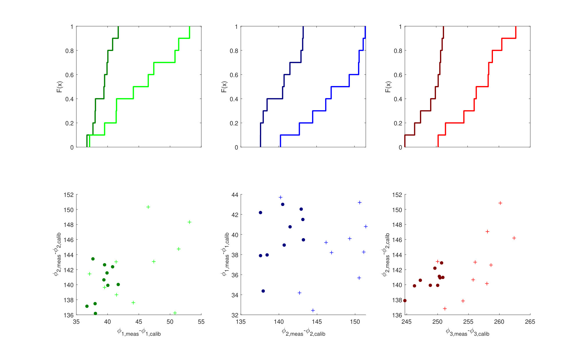 Figure 6
 Figure 7
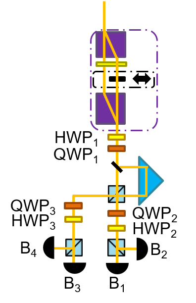 Figure 8
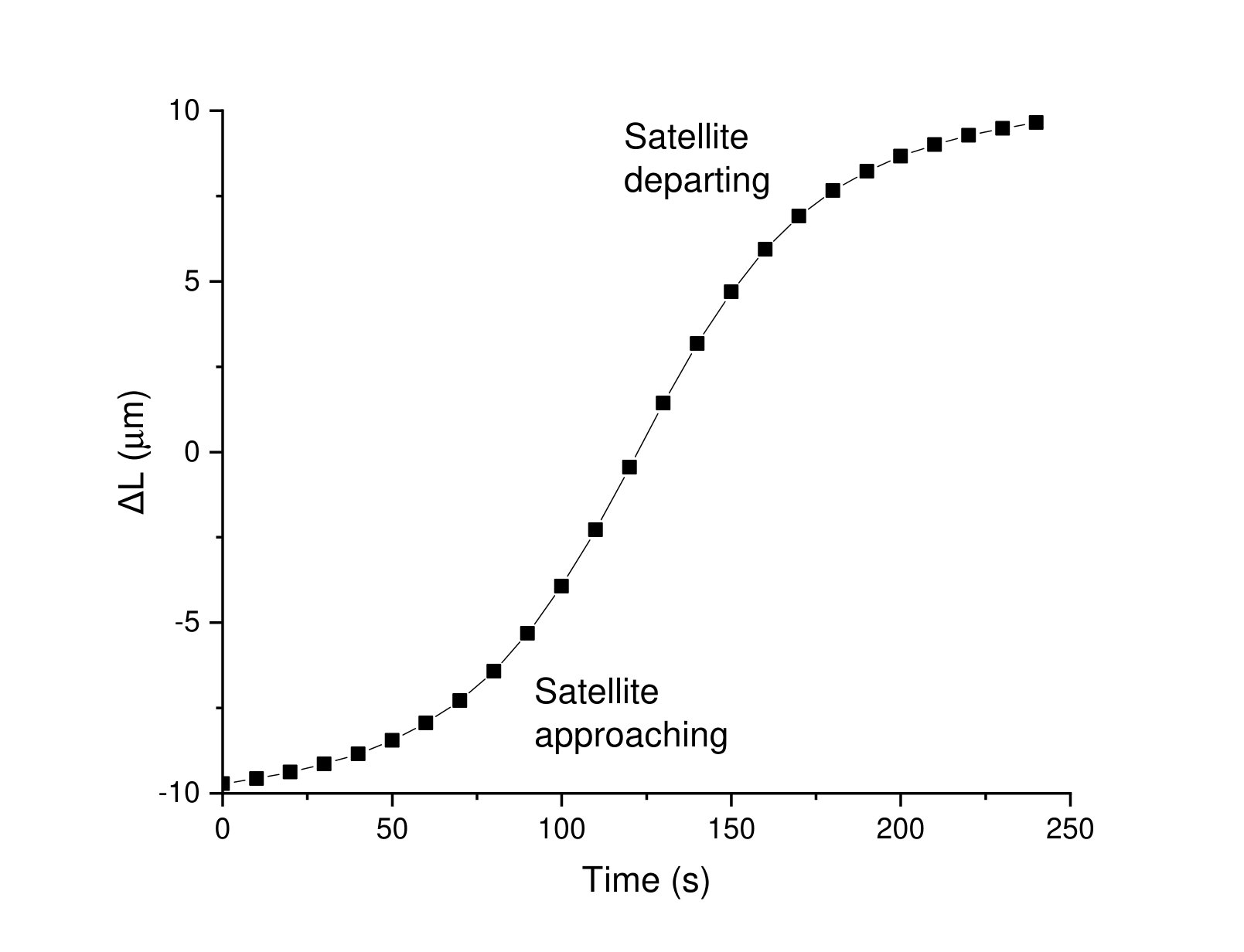 Figure 9
 Figure 10
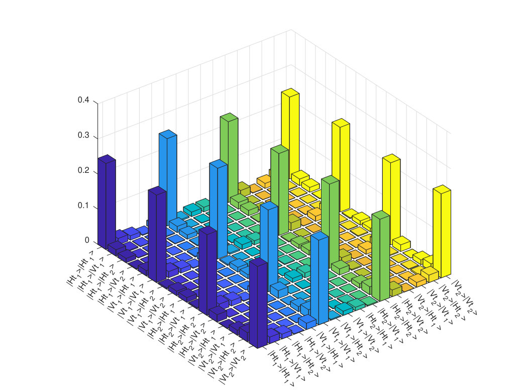 Figure 11
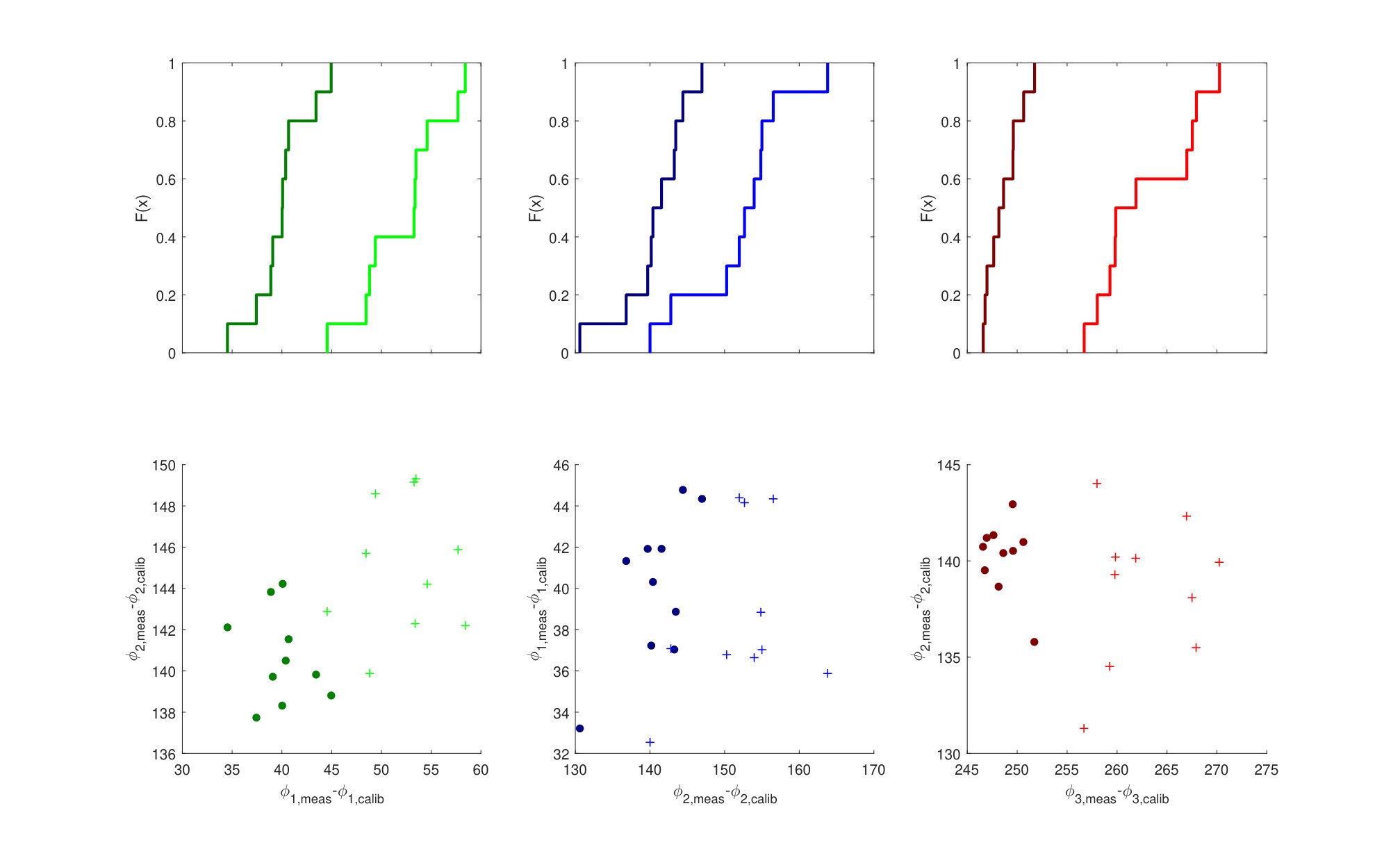 Figure 12
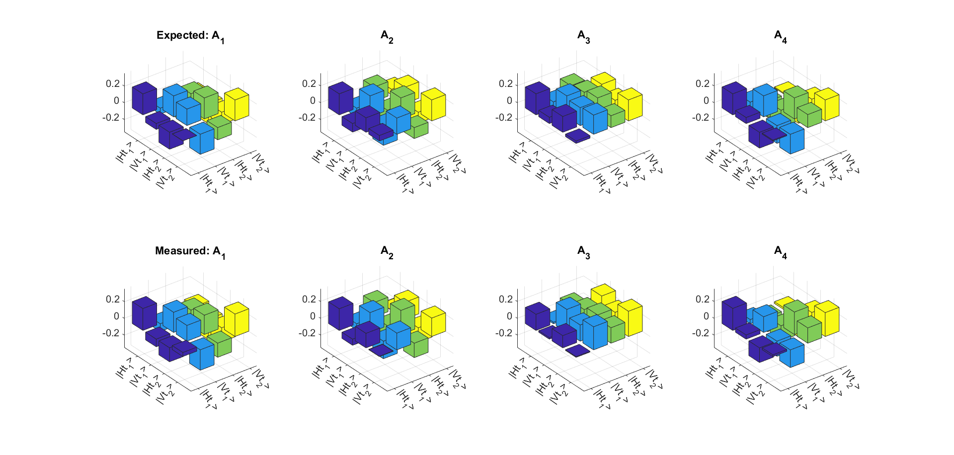 Figure 13
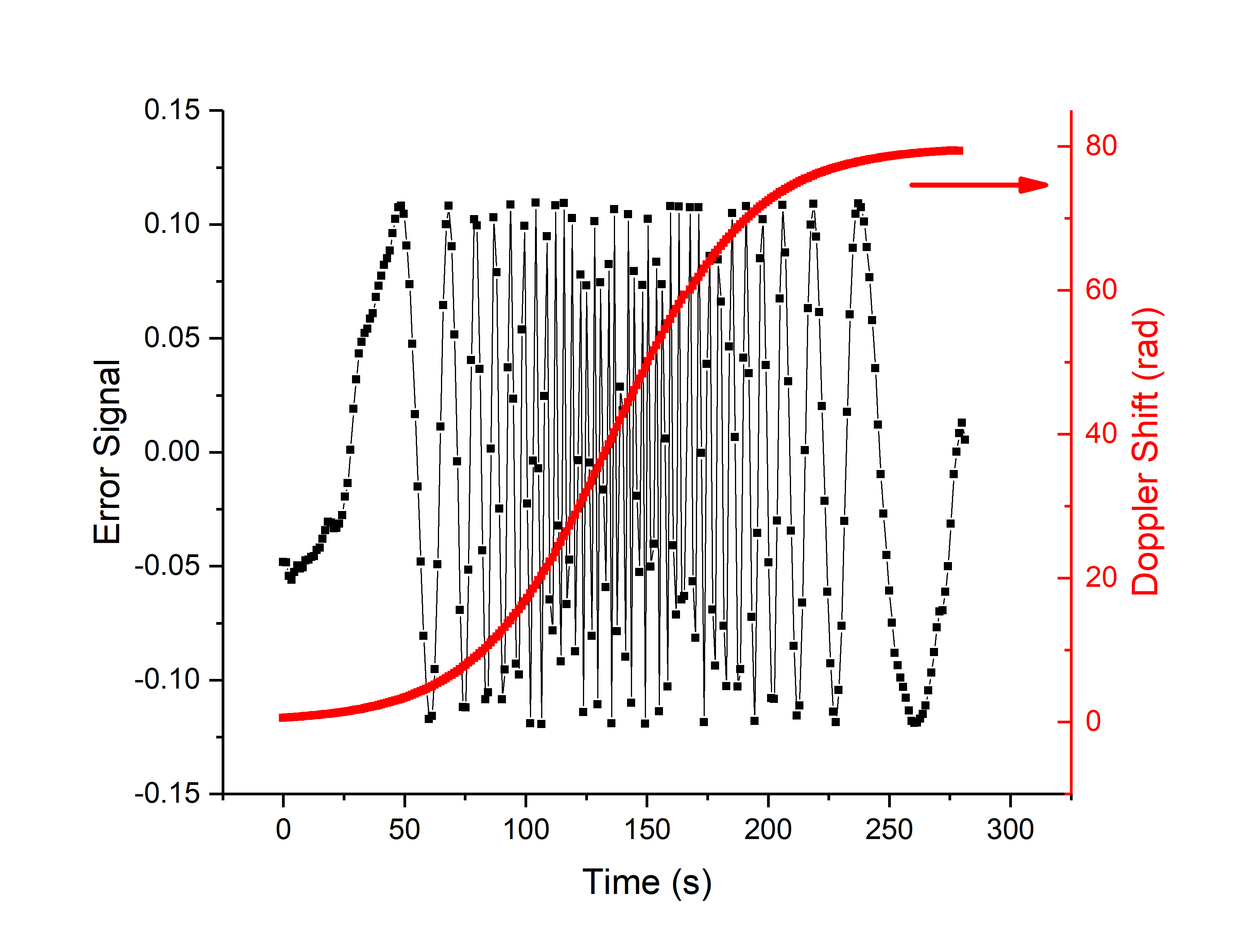 Figure 14
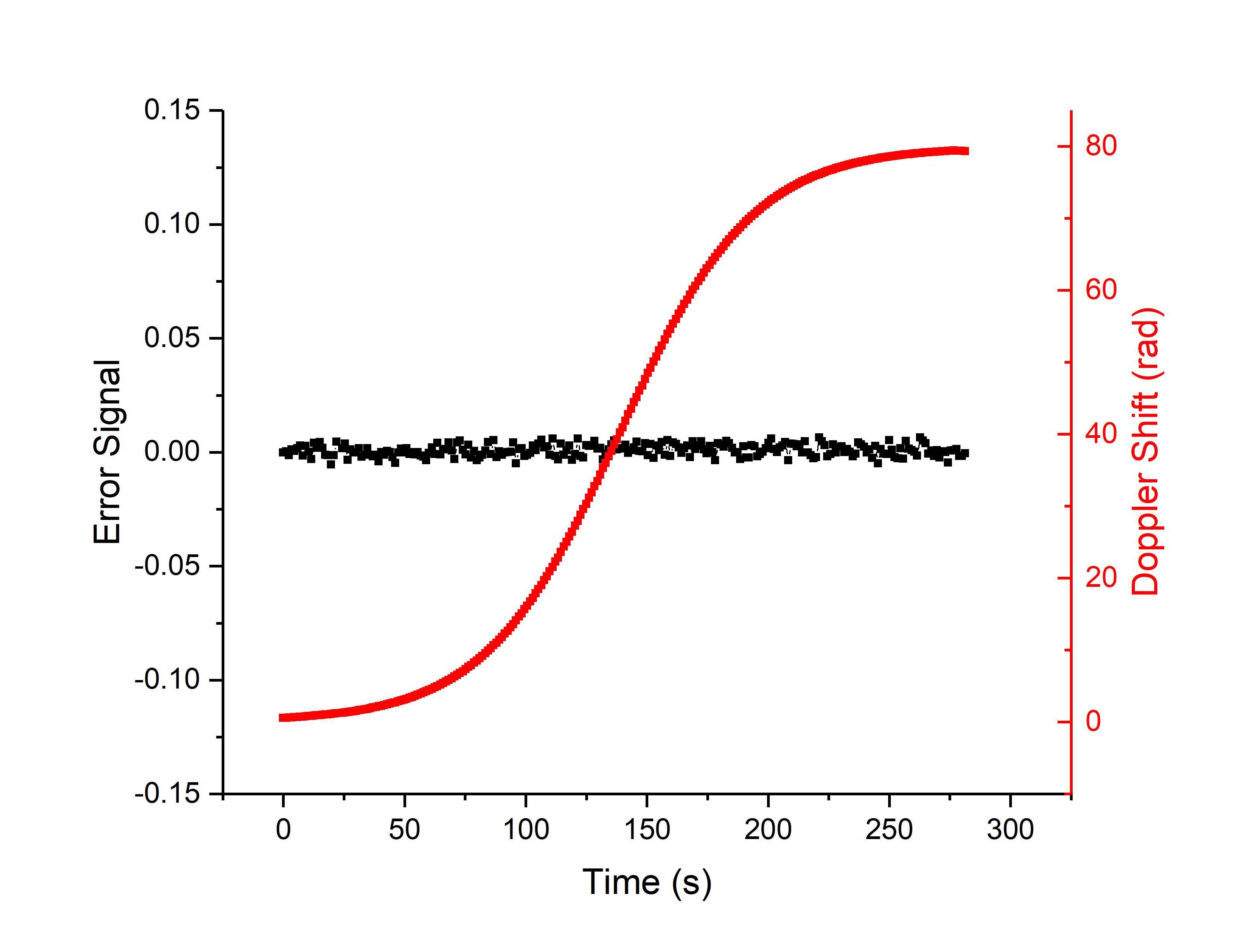 Figure 15
 Figure 16
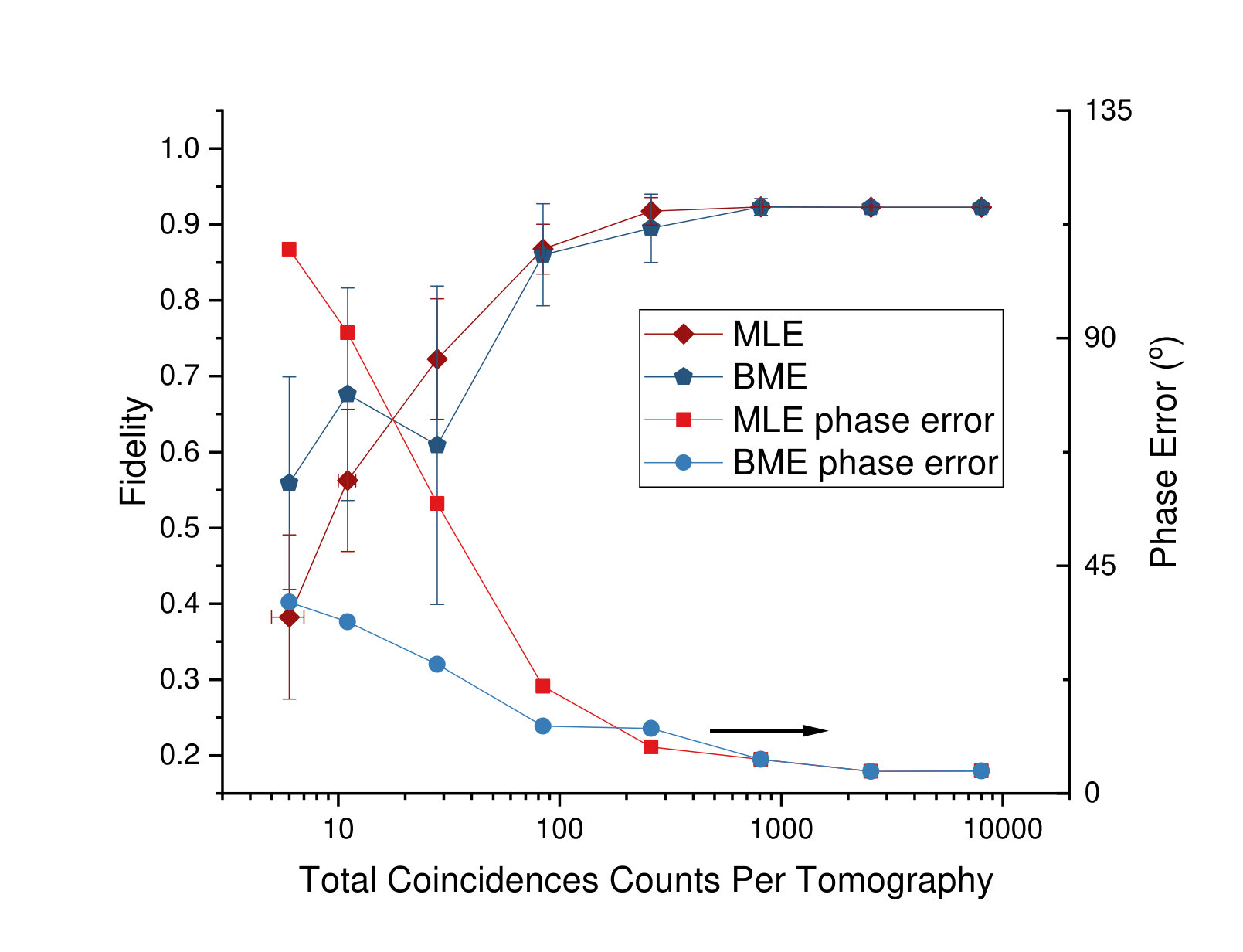 Figure 17
 Figure 18
 Figure 19
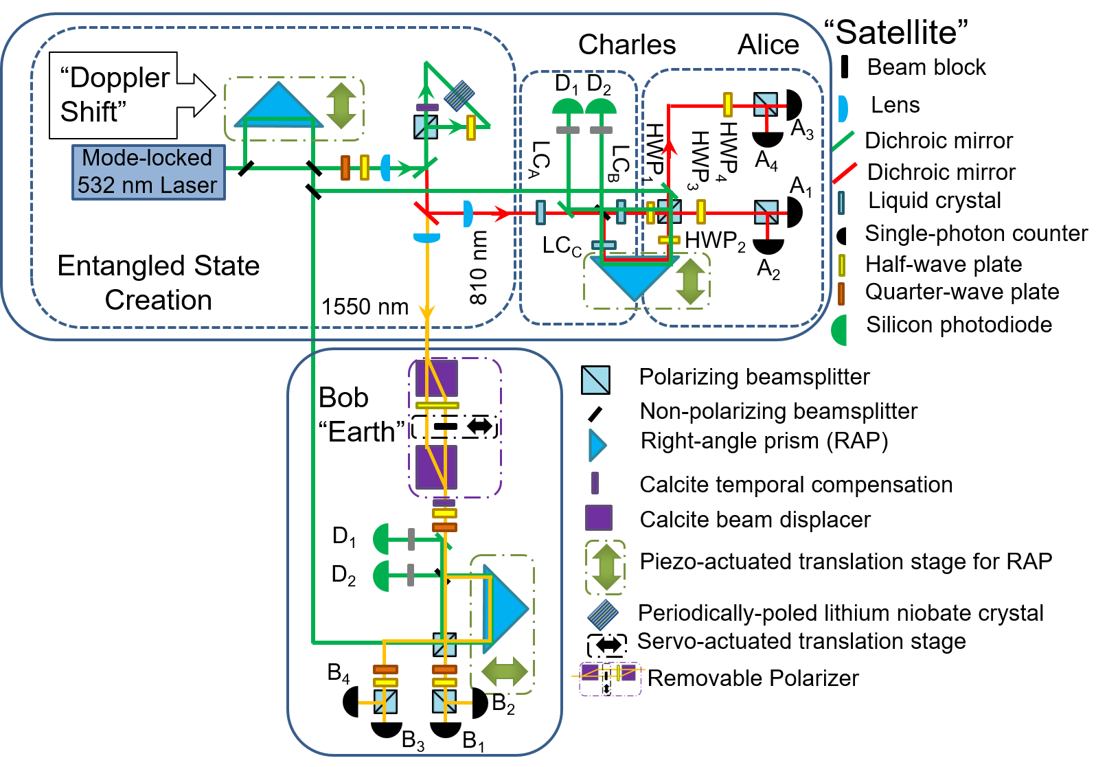 Figure 20
 Figure 21
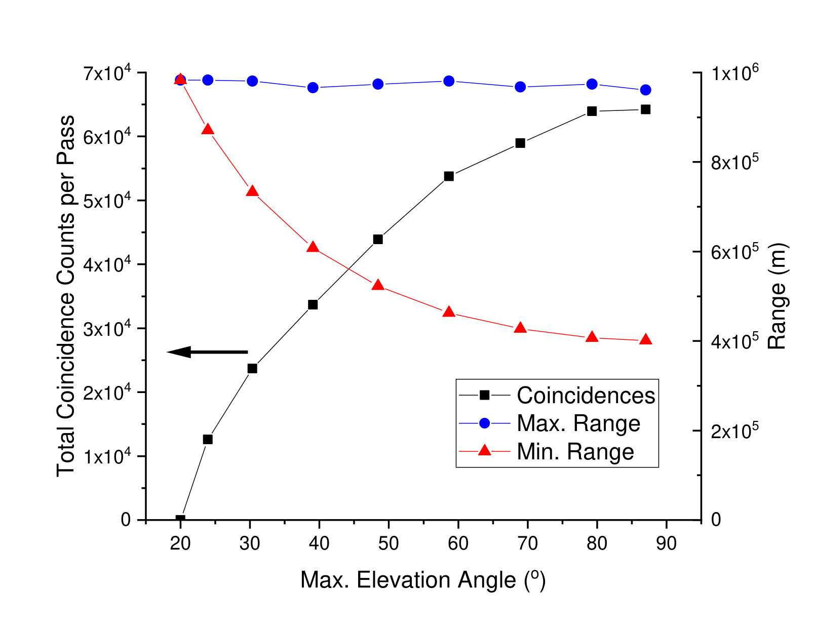 Figure 22
 Figure 23
 Figure 24
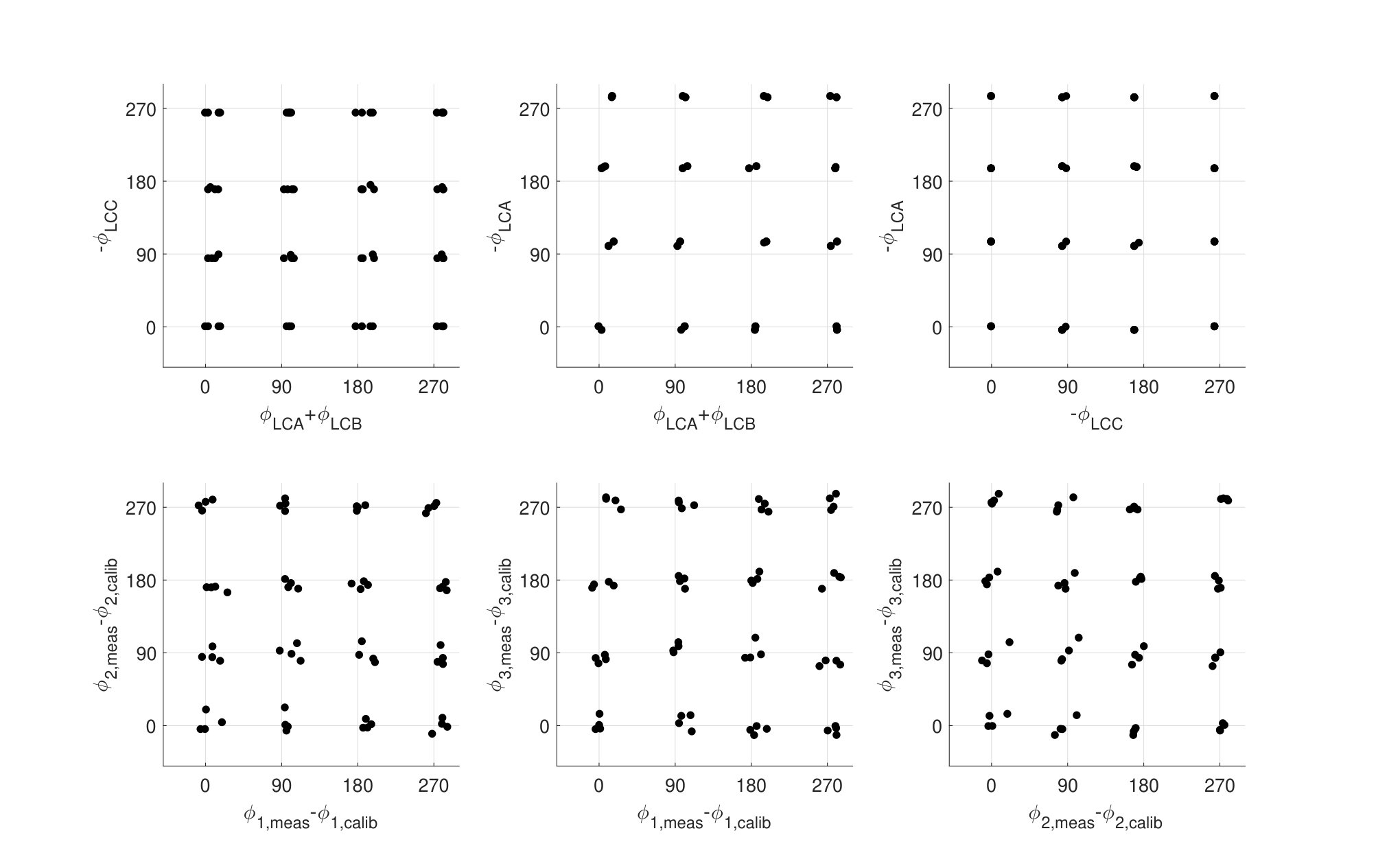 Figure 25
 Figure 45
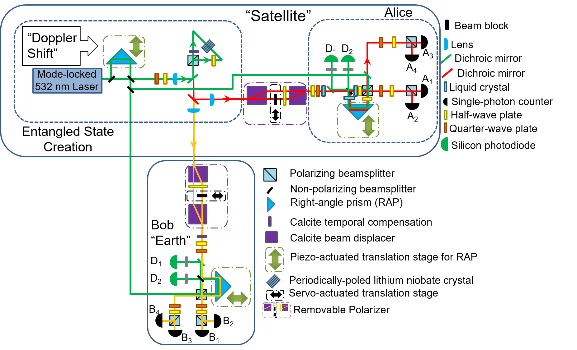 Figure 27
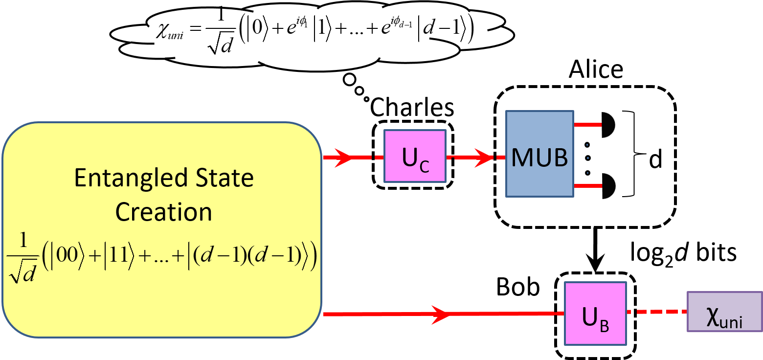 Figure 28
 Figure 29
 Figure 30
 Figure 31
 Figure 32
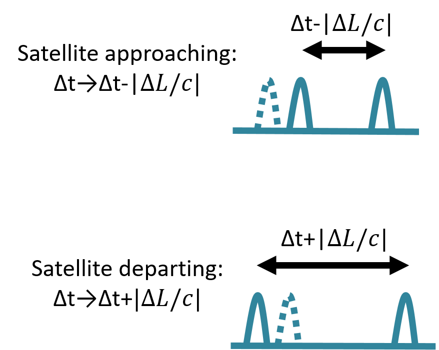 Figure 33
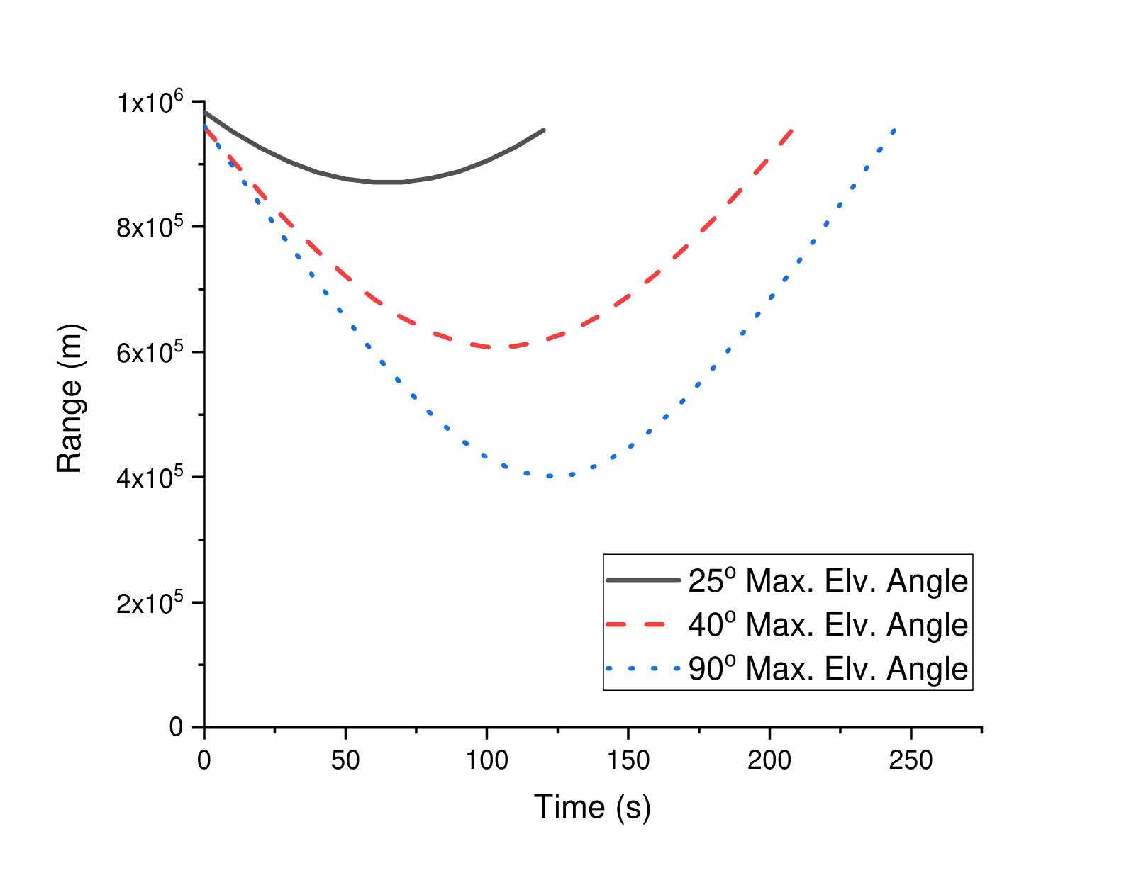 Figure 34
 Figure 35
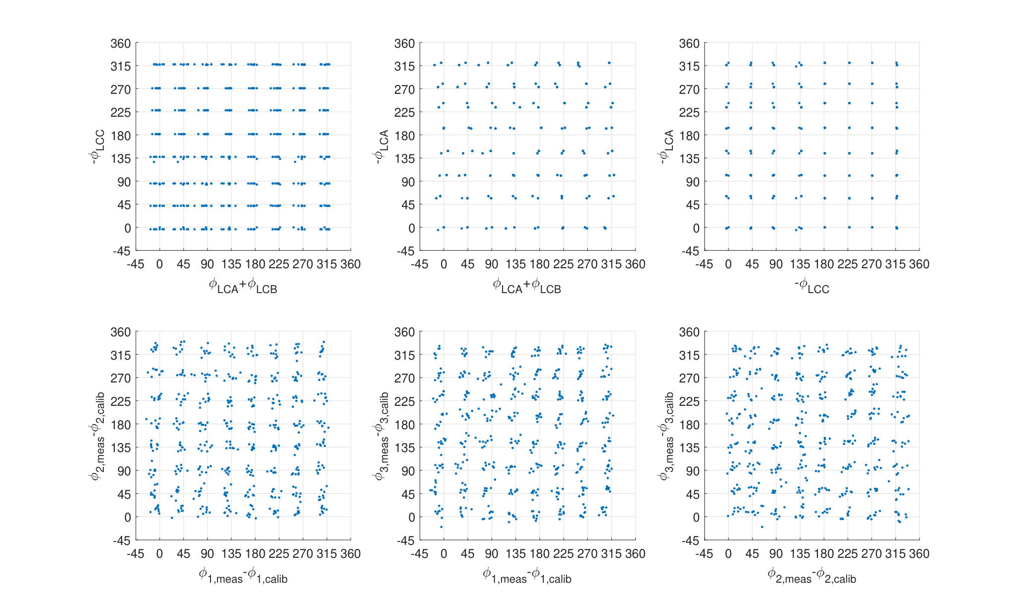 Figure 45
 Figure 37
 Figure 38
 Figure 39
 Figure 40
Peer Reviews
No public reviews on file for this paper yet. If you reviewed it on a platform where reviews are public (OpenReview, ICLR, NeurIPS, ICML), you can paste yours below so the community can read it here.
Videos
No videos yet. Explain this paper in a talk, walkthrough, or lecture? Add one.
Taxonomy
TopicsSatellite Communication Systems · Wireless Communication Networks Research · Advanced Wireless Communication Techniques
Time-bin and Polarization Superdense Teleportation for Space Applications
Joseph C. Chapman
Illinois Quantum Information Science and Technology Center, University of Illinois at Urbana-Champaign, Urbana, IL 61801
Dept. of Physics, University of Illinois at Urbana-Champaign, Urbana, IL 61801
Trent M. Graham
Dept. of Physics, University of Illinois at Urbana-Champaign, Urbana, IL 61801
Dept. of Physics, University of Wisconsin - Madison, Madison, WI 53706
Christopher K. Zeitler
Illinois Quantum Information Science and Technology Center, University of Illinois at Urbana-Champaign, Urbana, IL 61801
Dept. of Physics, University of Illinois at Urbana-Champaign, Urbana, IL 61801
Herbert J. Bernstein
Institute for Science & Interdisciplinary Studies & School of Natural Sciences, Hampshire College, Amherst, MA 01002
Paul G. Kwiat
Illinois Quantum Information Science and Technology Center, University of Illinois at Urbana-Champaign, Urbana, IL 61801
Dept. of Physics, University of Illinois at Urbana-Champaign, Urbana, IL 61801
Abstract
To build a global quantum communication network, low-transmission, fiber-based communication channels can be supplemented by using a free-space channel between a satellite and a ground station on Earth. We have constructed a system that generates hyperentangled photonic “ququarts” and measures them to execute multiple quantum communication protocols of interest. We have successfully executed and characterized superdense teleportation, a modified remote-state preparation protocol that transfers more quantum information than standard teleportation, for the same classical information cost, and moreover, is in principle deterministic. Our measurements show an average fidelity of , with a phase resolution of , allowing reliable transmission of distinguishable quantum states. Additionally, we have demonstrated the ability to compensate for the Doppler shift, which would otherwise prevent sending time-bin encoded states from a rapidly moving satellite, thus allowing the low-error execution of phase-sensitive protocols during an orbital pass. Finally, we show that the estimated number of received coincidence counts in a realistic implementation is sufficient to enable faithful reconstruction of the received state in a single pass.
I Introduction
A global quantum network would have myriad uses. For example, it could improve the collective computational power of quantum computers by allowing them to communicate Caleffi et al. (2018), enable arbitrarily long-distance secure communication using quantum cryptography Aspelmeyer et al. (2003), and might even facilitate planet-scale distributed quantum sensors, e.g., for clock synchronization Giovannetti et al. (2001), and super-resolution telescopy Gottesman et al. (2012); Khabiboulline et al. (2019a, b). Currently, the distance between nodes in a potential quantum network is limited by the absorption loss in fiber-optic cables or the effects of turbulence for free-space terrestrial channels. If a channel between a satellite and Earth were used as part of the network, the distances between nodes could be greatly increased because that channel is less affected by the above limiting factors Simon (2017). The utility of a free-space satellite-Earth channel has been recognized by many research groups around the world Khan et al. (2018). For example, the Chinese Micius satellite was used to demonstrate long-distance photonic-entanglement distribution Yin et al. (2017), one version of quantum key distribution (QKD) Liao et al. (2017, ), and a preliminary test of quantum teleportation Ren et al. (2017). Additionally, there is significant work ongoing in Singapore Grieve et al. (2018), Italy Vallone et al. (2015), Canada Pugh et al. (2017), and Austria Steinlechner et al. (2017); Liao et al. .
To further the development of quantum communication applications in space, we have created a system that can execute multiple quantum communication protocols, including high-dimensional entanglement-based quantum key distribution Chapman et al. (2019), superdense teleportation (SDT) Bernstein (2006), and high-dimensional Bell inequality and quantum steering tests Zeitler et al. . With additional modifications, the system could be suitable for operation on a satellite. In this work, we characterize our source of hyperentangled photons and the performance of SDT in our system over its whole message space, and demonstrate through lab test and calculation the ability to robustly execute SDT during a single orbital pass of a low-earth orbit satellite, e.g., the International Space Station (ISS). This work significantly exceeds previous SDT work Graham et al. (2015) by the authors, due to incorporation of robust quantum degrees of freedom/elimination of encoding in non-robust degrees of freedom, compensation for the Doppler shift (which otherwise renders the protocol useless), and a more thorough characterization of the SDT system in general; we have also incorporated a comparison between the standard Maximum Likelihood analysis and Bayesian analysis methods that are superior to standard quantum state tomography techniques for low-rate communications. Finally, for the first time we have undertaken a thorough analysis to project rates and performance in a low-earth-orbit demonstration of this protocol.
II Superdense Teleportation Protocol
SDT, as shown in Fig. 1, is a three-party protocol involving Alice, Bob, and Charles. Charles wants to send Bob an “equimodular” quantum state—a subset of the states in the available Hilbert space, in which all terms have the same magnitude:
[TABLE]
for any values of , , . To begin the protocol, Bob and Charles share a d-dimensional maximally entangled state:
[TABLE]
onto which Charles locally encodes his desired phases:
[TABLE]
Next, Alice measures Charles’ photon in a mutually-unbiased basis from the one in which Charles applied the phases, e.g., the basis
[TABLE]
where we now restrict our discussion to d=4, relevant for our experimental implementation. States to are those projected onto by Alice’s 4 detectors. Before Alice’s measurement, the full state of the system is given by
[TABLE]
Upon measurement, Alice sends her result to Bob (using 2 classical bits of information), who then applies the correct unitary transformation (a phase shift on one of the four terms) so that Graham (2016)
[TABLE]
Although the SDT state space is restricted to equimodular states, and is therefore not suitable for general quantum computation, these states are sufficient to enable blind quantum computing, a client-server cluster quantum computing model that ensures privacy of the inputs, the outputs, and the computation being performed Broadbent et al. (2009). Moreover, the SDT protocol is deterministically successful, in contrast to quantum teleportation and probabilistic remote state preparation, which both only succeed at most half of the time using linear optics Graham et al. (2015). In addition, it also uses fewer classical communication resources than quantum teleportation and deterministic remote state preparation Graham et al. (2015); for example, whereas standard teleportation requires Alice to send 2 classical bits to teleport a single qubit (described by two continuous variables, e.g., ), SDT transmits three continuous variables for the same two classical bits. Higher-dimensional quantum teleportation has been performed before but with lower fidelity and only probabilistic success Wang et al. (2015); Luo et al. . Furthermore, Alice’s measurements for SDT are substantially less resource intensive than those needed, e.g., for remote state preparation Graham et al. (2015); this is an important consideration for a satellite-based protocol.
III SDT Protocol Execution
Superdense teleportation has been executed previously using photons hyperentangled in their polarization and orbital angular momentum (OAM) Graham et al. (2015). For our intended goal of transmitting quantum information over a channel from space to earth, time bins are a much better choice than OAM modes, as the latter are corrupted by atmospheric turbulence and require larger apertures to faithfully detect Torres (2012). Using nondegenerate spontaneous parametric downconversion, our source produces time-bin and polarization entangled photons (see Appendix A) in the 16-dimensional equimodular state
[TABLE]
Here H and V refer to horizontal and vertical polarization, and refer to two time bins, and 810 and 1550 (nm) are the photon wavelengths. As shown in Fig. 2, the 810-nm (1550-nm) photon is distributed to Charles (Bob), who applies phases , , and on the state by actuating 3 different liquid crystals, , , and , to allow arbitrary phase selection over the range . Alice’s projective measurement in a mutually unbiased basis is carried out by the polarizing beamsplitter (PBS) of her interferometer, preceded by and in the interferometer arms, which effectively place the PBS into the diagonal/anti-diagonal basis. Similarly, and are oriented at 22.5*∘* with respect to horizontal, so the detectors project onto a superposition of time bins. Instead of having Bob complete the protocol by making the necessary unitary transformation, Bob measures 4 tomographies, conditioned on which of Alice’s detectors fires. This allows us to tomographically reconstruct all 4 of the different states sent to Bob and apply the unitary transformation during the analysis after state reconstruction.
IV Results
To verify the quality of our source, we performed a full tomography of the joint state of the system by performing 1296 measurements (6 measurements for each qubit in the ququart). This involved adding extra half- and quarter-wave plates and a removable polarizer into Alice/Charles’ side so a complete tomography could be made on each photon of the pair; see Appendix D.4 for details. The purity of the reconstructed density matrix (Fig. 3) is ; the fidelity of the absolute value of the reconstructed density matrix, , with Eqn. 10 is
[TABLE]
For each calculation, the error bar was produced from a Monte Carlo analysis, assuming Poissonian counting statistics and using 100 samples, with mean count values on the order of the number of detected events for each of the tomography measurements (See Appendix D, Table 3) .
IV.1 Phase Space Characterization
To characterize the performance of the SDT protocol over the complete space of possible states (any value of , , and ), we measured every combination of , , and at roughly intervals between . These 512 states are represented in phase space in Fig. 4 for trials where Alice obtained a click at detector (which is representative of events detected by the other three detectors). More precisely, the plots show the difference between the phases of the reconstructed state (, , and ) and the calibration phases (, , and ) from a calibration tomography taken every 4 tomographies. The phases between the polarizations are relatively stable and do not need to be measured except when the alignment changes, but the time-bin phase is more susceptible to slight phase drift. We believe the increased variation in (top left graph of Fig. 4) is due to the compounded variation in and as , the phase which changes within each grouping in the projections of Fig. 4, is increased. The average fidelity over the entire grid and all of Alice’s detectors is
[TABLE]
where and
[TABLE]
Here
[TABLE]
From the grids in Fig. 4, we calculate the standard deviation of , averaging over all three phases, to be , while the mean is only . We estimate of the standard deviation is from Poisson statistical fluctuations and alignment drift in the setup over time.
To further assess errors, we repeated the measurement 8 times for every combination of , , and at roughly intervals between ; allowing us to plot a grid of the average phase measured at each point (see Appendix D, Fig. 10). From these data, we calculate the mean and standard deviation of to be and , respectively. Additionally, the average fidelity of the measured state with each target over the entire grid, including all 4 of Alice’s measurement outcomes, is . We identified some of the causes of infidelity in our system to be imperfect phase setting, imperfect phase stabilization, different measurement efficiency for the different tomography measurements, and non-equal magnitudes of the terms in the superposition; see Appendix D.3 for quantitative estimates of these effects.
In order to further assess the resolving power of our system to distinguish states with nearby phase values, for each phase (, , and ), we created two distributions (two liquid crystal settings) of 10 samples each, corresponding to phases differing by on average; we then applied a two-sample Kolmogorov-Smirnov (KS) test Kolmogorov (1933) to test the null hypothesis (once for each phase) that all 20 samples were from the same distribution (liquid crystal setting), concluding that we can reject the null hypothesis that the data are drawn from a single distribution with , in other words, with a 5 probability of wrongly rejecting the null hypothesis; see Appendix F for more information. Thus, we can estimate the total number of resolvable teleported quantum states with our system to be .
IV.2 Doppler Shift Compensation
Because a low-earth orbit (LEO) satellite travels at km/s, the source will have moved non-negligibly between the times when the early and late time-bins are transmitted. As the satellite approaches (recedes) this shortens (lengthens) the interval between emitted time bins from the Earth’s reference frame. Uncorrected, the corresponding variation in phase (between the first two and last two terms in the state from Eqn. 10) would completely obscure the phases Charles is attempting to teleport to Bob: a variation of about 80 radians is expected, depending on the time-bin separation and the orbit elevation angle. See Appendix G for more information. To keep this Doppler shift (and any other time-varying phase shifts) from adversely affecting the protocol’s performance, we developed a phase compensation system that uses a classical laser beam and proportional-integral feedback Minorsky (1922) to stabilize the path-length difference of the interferometers. Figure 5 shows the performance of the classical stabilization system while a continuously-varying, lab-simulated Doppler shift, matching that expected in a typical satellite orbit, was imposed. The standard deviation of the phase with the stabilization active is .
We measured 9 tomographies while executing SDT for the same choice of , , and . Without phase stabilization, we obtained an average fidelity ; with the phase stabilization turned on, we obtained an average fidelity and had a standard deviation of . We suspect the cause of the increased phase variation during the Doppler shift to be relative drift between the pathlengths of Alice and Bob’s interferometers while the Doppler shift is taking place. This should not occur during an actual implementation in space, because a Doppler shift would not occur on the time bins sent from the pump to Alice/Charles’ interferometer (which is on the same platform as the source); only those sent to Bob’s interferometer would experience a Doppler shift.
IV.3 Link Analysis
The maximum elevation angle of a LEO satellite with respect to a ground station on earth varies from pass to pass, and the instantaneous elevation angle (defined as the angle between the horizon and the satellite) changes as the satellite passes overhead, leading to a change in the separation between the satellite and ground terminal — the “range” (Fig. 6a). With that in mind, displayed in Fig. 6b, we calculate the estimated total coincidence counts per pass, maximum range per pass, and minimum range per pass versus maximum elevation angle per pass, assuming the minimum acceptable elevation angle during a pass is (which fixes the maximum range to around m, as seen in Fig. 6b). For these calculations, we used simulated orbit data for all orbital parameters—the simulated satellite orbit had a 400-km altitude and inclination (appropriate, e.g., for the ISS), and the range as a function of time was calculated from the satellite to a ground station located at N latitude; see Fig. 6a for example data. The Friis equation () to estimate channel transmission as a function of range Friis (1971); Alexander (1997) was numerically integrated over the whole pass (for transmitting telescope diameter m, receiving telescope diameter m, and wavelength nm, with the added assumptions of a 6-dB loss for combined receiver telescope Biswas et al. (2014) and adaptive optics system single-mode fiber collection efficiency Chen et al. (2015), and 4-dB loss for an estimate of the analysis/detection system transmission), and assuming a 400-MHz repetition rate pump laser, pair production probability of 0.01 per pump pulse, and a 4-dB loss from the analysis/detection system in space. This experiment would require an adaptive optics correction system so the collected light can be efficiently coupled into a single-mode fiber before entering Bob’s analysis/detection system. With this requirement, any turbulence is effectively converted to a reduction in transmission.
All tomographies analyzed thus far in the paper used maximum-likelihood estimation (MLE) James et al. (2001). We also analyzed some tomographic data using a Bayesian-mean-estimation (BME) approach Granade et al. (2016), computing the representative state as an average over all states, weighted by the likelihood that a state produced the data observed. Using MLE yields results that are biased towards pure states Ferrie and Blume-Kohout (2018), and this effect becomes more significant when the data used for the tomography has fewer counts, as can be seen in the low count regime in Fig. 7. In these low-count regimes, using BME leads to results that are more reflective of the data measured. However, analyzing tomographic data using BME is more computationally intensive, especially when more than several hundred coincidence counts are collected, so MLE is often preferred with higher counts because the resultant difference between BME and MLE becomes small.
SDT is not inherently affected by source brightness except for slight degradation in purity from multiple pair events Chapman et al. (2018); however, to verify that the protocol is operating successfully, one needs to take a tomography of the received photons contingent on which state Alice measured (-); such conditional tomography is required because we are not yet implementing the final active feedforward step of the full SDT protocol. We know from previous analysis Chapman et al. (2018) that only coincidence counts total per the 36 tomography measurements are needed for a reliable reconstruction (state Fidelity ) using MLE. From our calculations above, all passes above 25*∘* maximum elevation angle should produce more than 10,000 total coincidence counts per pass (Fig. 6). Therefore, under those assumptions, a future implementation of this system in space should produce and measure more than enough coincidences to verify an implementation of SDT in a single pass. Furthermore, with currently available technology, such as adaptive optics on receiver telescopes for single-mode fiber coupling, active polarization compensation to ensure Bob and Charles have a common basis, and time-bin phase stabilization as demonstrated in this work, SDT should be implementable in a space-to-earth channel without degradation compared to our laboratory implementation.
V Conclusions
We have shown a systematic characterization of our system to execute SDT, and characterize the full volume of accessible quantum states by measuring the fidelity of states at regular intervals of phase. The phase error was measured from this characterization, along with the distinguishability of closely spaced phases. We also demonstrated the ability to operate during a Doppler shift by employing an active feedback system. Lastly, we calculate the expected coincidence counts for a range of satellite orbital passes and show that for nearly all of them we should have ample counts to reconstruct the received state faithfully.
The value in quantum communication occurs when two remote parties can coordinate to achieve some desirable task beyond the capabilities of classical communication. Because SDT transmits only a restricted space of states, one might worry that the protocol would be insufficiently versatile to enable interesting or useful quantum processing tasks. However, the equimodular states of SDT enable high-dimensional entanglement-based quantum cryptography Chapman et al. (2019); moreover, they are just the type required for quantum fingerprinting Buhrman et al. (2001) and for blind quantum computing Broadbent et al. (2009). Therefore, a space-to-earth implementation of SDT would be an enabling demonstration along the path toward a useful global quantum network.
VI Acknowledgements
The authors acknowledge Alexander Hill for the suggestion to use a 2-sample KS test. Thanks to MIT-Lincoln Laboratory for the orbital simulation calculations. This work was primarily supported by NASA Grant No. NNX13AP35A and NASA Grant No. NNX16AM26G. This work was also supported by a DoD, Office of Naval Research, National Defense Science and Engineering Graduate Fellowship (NDSEG).
VII Author Contributions
All authors contributed to experiment design and commented on manuscript. H.B. conceptualized SDT protocol. T.G. constructed the initial optical system and wrote the preliminary version of the tomography analysis code. C.K.Z. started upgrade of detection system, implemented Bayesian analysis, and calculated the tomography settings and the contributions to the loss of fidelity. J.C.C. upgraded the optical system and finished upgrade of detection system, and carried out all experiments and MLE data analysis. J.C.C., C.K.Z., and P.G.K. wrote the manuscript.
Appendix A State Generation and Detection
To create the photons entangled in polarization and time bin, an 80-MHz mode-locked 532-nm laser (frequency doubled from 1064 nm, Spectra Physics Vanguard 2.5W 355 laser) with a pulse width 7 ps was sent through a 2.4-ns delay to split every pump pulse into an early and late pulse, each of which coherently pumps the polarization entanglement source Marcikic et al. (2002), a polarizing Sagnac interferometer with a Fresnel rhomb (used as a broadband half-wave plate), type-0 periodically poled (poling period is 7.5 m) lithium niobate crystal, and a calcite crystal (to compensate for dispersion); the horizontal (vertical) component of the diagonally polarized pump travels (counter)clockwise through the Sagnac. Neglecting time-bins, traversing the two paths of the interferometer corresponds to this transformation Shi and Tomita (2004); Kim et al. (2006):
[TABLE]
where the subscripts are nominal central wavelengths of the photons. Sending a superposition of time bins into the polarizing Sagnac results in the state Eqn. 10 of the main text.
The 532-nm pump bandwidth is 64 GHz. The downconversion bandwidth was measured by stimulated downconversion (difference-frequency generation) between a tunable 1550-nm laser and the pump Zielnicki et al. (2018). The tunable 1550-nm laser was swept and a peak in the collected 810-nm counts was recorded. The peak was centered at 1551 nm (corresponding to 809.7 nm for the conjugate photons), with a full-width at half-maximum width of 1.5 nm (0.4 nm) Graham (2016).
Due to birefringence, and do not exit the Sagnac source at exactly the same time. To compensate for this we inserted 0.5-mm of a-cut calcite into the 1550-nm beam path. This increased the visibility in the diagonal polarization basis from 91% to 98%.
For Charles to encode his desired phases, he used , , and , with their fast axes located along the horizontal, horizontal, and vertical axes, respectively, to allow arbitrary phase selection over the range .
The 810-nm photons were detected by 4 avalanche photodiodes (Excelitas SPCM-AQ4C) with efficiency 45%. The 1550-nm photons were detected by 4 1550-nm-optimized WSi superconducting nanowire detectors from NASA’s Jet Propulsion Laboratory, with efficiency 80% Chapman et al. (2017); Bob’s detector B2 had an efficiency of 40% due to coupling fiber misalignment after installation. The outputs of the detectors were collected by a timetagger with 156-ps resolution (UQDevices UQD-Logic-16). The symmetric heralding efficiency into single-mode fiber was 0.01, when including the above detection efficiency, analysis/detection system transmission ( 0.3), and entangled-photon-source collection efficiency into single-mode fiber ( 0.13).
Appendix B Time-bin Phase Stabilization
Due to environmental disturbances, temperature fluctuations, and the simulated Doppler shift, it was necessary to implement an active phase-stabilization system to simultaneously stabilize the phases between and in both Alice/Charles’ and Bob’s analyzer interferometers, relative to the pump interferometer. We directed some of the pump light, exiting the unused port of the pump delay interferometer, into the analyzer interferometers (see Fig. 2). The pump light was vertically displaced from the 810-nm photons so it would not propagate through the liquid crystals and receive a phase shift. The light was detected by and , low-bandwidth, amplified Si photodiodes (Thorlabs PDA36A), at both output ports of each interferometer. An error signal was calculated from the photodiodes:
[TABLE]
The factor is necessary to balance the different visibilities measured in each output port, since the optics used in the analyzer are designed for the downconversion wavelengths and not the stabilization wavelength. For each analyzer interferometer, this error signal was input to a Proportional-Integral (PI) feedback algorithm with a set-point of zero and an output rate of 100 Hz. The PI algorithm output was fed to a driver to actuate a piezo-electric crystal on the translation stage of the right-angle prism inside the corresponding analyzer interferometer.
Appendix C Time-Bin Filtering
None of the the detectors used in this experiment were gated internally, allowing photon detection at any time. Initially, this presented a problem because there are three pulses emitted from Alice’s and Bob’s analyzer interferometers. For this experiment, it was necessary to implement a circuit to filter out events from the outer two pulses, because only the middle pulse contained events with a superposition of time bins. Each pulse emitted from the interferometer has a fixed delay with respect to the input pulse, so employing an AND gate between each detector and the laser clock (with an adjustable delay) created a time filter with a width of 1 ns centered around the middle pulse Chapman et al. (2019).
Appendix D Tomographic Reconstruction
To reconstruct the state of the photons received by Bob, 36 different measurements were made by rotating the waveplates, moving the removable polarizer (some settings required a certain polarizer; see Table 2), and recording the coincidences between Alice and Bob’s detectors.
The measurements performed using the setup in Fig. 8 were:
[TABLE]
where D(A) is (anti-)diagonal polarization and R(L) is right(left) circular polarization. These measurements form an informationally overcomplete set in the space of interest; after data collection, they were analyzed to produce 4 density matrices (1 for each tomography conditional on which of Alice’s detectors fired) using maximum-likelihood estimation James et al. (2001).
To measure states in the first group of measurements in Eqn. 19, and are rotated to 0*∘* or 45*∘* to project the detectors onto one time bin or the other but not superpositions of them. and in front of the interferometer are used to change what basis the PBS in the interferometer projects on to. To measure states in the second group, the beam block in the removable polarizer moves to block the orthogonal polarization. The polarization is rotated into the D/A basis and and are rotated to 22.5*∘, so the detectors project onto superpositions of the time bins. Also, to maintain the same level of phase sensitivity across all measurements, the count time is doubled since the polarizer blocks roughly half the photons. For measurements of the third and fourth groups, and are rotated to put the PBS in the correct basis and and are rotated to 22.5∘* as before. To change the phase shift between and , and are rotated. See Table 2 for exact settings.
D.1 Tomography Measurement Efficiency Calibration
There were 4 tomographies measured simultaneously, each conditional on one of Alice’s 4 detectors. Additionally, there were 4 different simultaneous measurements because all 4 of Bob’s detectors projected onto a different state during the 9 different settings for the wave plates and polarizer. To allow the use of all four of Bob’s detectors for a single tomography, a measurement efficiency calibration was made periodically so the differences in the path and detection efficiencies for - could be normalized to Bob’s detector . We calibrated the measurement efficiency of every measurement in the tomography with respect to detector . This calibration consisted of five tomographies with 36 measurement settings. From these tomographies, we are able to calculate the average measurement efficiency ratio between taking the measurement with detector and one of the other three detectors (see the four right-most columns of Table 1). Table 1 shows the exact mapping between the states measured in the 9- and 36-setting tomographies. A complete efficiency calibration of Bob’s and Alice’s measurement systems was not carried out throughout the experiment. Therefore, all tomographies measured include effects from the measurement efficiencies (from the different paths) to Bob’s detector (- were normalized to ) and the measurement efficiencies for Alice’s detectors. We are able to reduce adverse effects on the measured fidelity to by balancing the measurement efficiencies using detector alignment and by adjusting the relative probabilities for the terms in our equimodular state. Without this balancing, the fidelities would have been degraded by to . Effectively, the states that result from our tomography are the states collected by our detectors, not the states that enter our measurement system. Equivalent results would have been obtained for the reconstruction of states that enter our measurement system if a complete system efficiency calibration had been carried out so that the differing path efficiencies could be normalized away and the state creation elements were rebalanced accordingly.
D.2 MLE Optical System Representation
For maximum-likelihood state estimation, the optical system is simulated using Jones calculus and is operated on a density matrix with optimizable parameters James et al. (2001). The density matrix, , is constrained to represent a physical state using a Cholesky decomposition:
[TABLE]
where
[TABLE]
We represented the optical system making the measurement as
[TABLE]
where
[TABLE]
[TABLE]
[TABLE]
[TABLE]
[TABLE]
[TABLE]
[TABLE]
,
[TABLE]
[TABLE]
, , are the angles of half-wave plates 1-3, and , , are the angles of quarter-wave plates 1-3. and are the transmission settings of the removable polarizer; for example, if and , the removable polarizer is positioned such that is transmitted while is blocked. The angles and positions of these elements during a tomography are listed in Table 2.
D.3 Representative Data and Error Analysis
The real parts of the density matrices of the expected and received states for a typical superdense teleported state are shown in Figure 9. The received states were reconstructed from the data in Table 3. This data was taken while counting for 15 seconds for each setting, except the settings that used the movable polarizer in front of Bob’s interferometer (9-settings # 1-2, 36-settings # 1-8), which used a count time of 30 seconds. The pump power was 0.5 mW at the PPLN crystal.
From measurements of components in our system and detailed numerical simulation, we find drop in fidelity from imperfect polarizer extinction ratios, from imperfect LC basis and phase settings, from unbalanced measurement efficiencies, from imperfect time-bin qubit purity, and from imperfect H/V and D/A visibility in the removable polarizer.
D.4 Full State Tomography
To measure the total joint state of the entangled photon pairs, a few additions were made to the system to allow a tomography to be measured on Alice/Charles’ photon: a half- and a quarter-wave plate were added before Alice/Charles’ interferometer and then a quarter-wave plate was added to each output port of the interferometer; additionally, a removable polarizer was added before the interferometer. The setup diagram during this measurement is in Fig. 11. The tomography was measured using 36 (Alice’s/Charles’ settings) x 36 (Bob’s settings) = 1296 settings.
Appendix E Liquid Crystal Calibration
To calibrate the phase applied by each liquid crystal for each driving voltage, a tomography was measured on Bob’s photon (as above) conditioned on detection of Alice’s photon by detector ; the phase between H and V was then extracted from the density matrix. This is distinctly different from the phase extraction used in the analysis of the SDT protocol trials—in that case all phases were extracted, including between the time bins. Here, effectively only a polarization tomography is conducted to measure the phase between H and V applied by the liquid crystal. Additionally, to reduce phase error as much as possible, it was necessary to periodically ( 2 days) recalibrate the phase applied by the liquid crystals as measured from the tomography system. Otherwise a drift as much as is observed, due to an induced change in the phase extraction from a varying measurement-efficiency imbalance. The tomography involves many projective measurements, each with a different efficiency, and such differences can modify the extracted phase values.
Appendix F Two-sample KS tests
In order to assess the resolving power of our system to distinguish states with nearby phase values, for each phase (, , and ), we created distributions for two closely spaced phase settings (two liquid crystal settings) of 10 samples each; we then applied a two-sample Kolmogorov-Smirnov (KS) test Kolmogorov (1933) to test the null hypothesis (once for each phase) that all 20 samples were from the same distribution (liquid crystal setting). The distributions and their empirical cumulative distribution functions (CDF) are shown in Fig. 12. These distributions had a standard deviation of and were, on average, separated by The two-sample KS test statistic is
[TABLE]
where and are the empirical distribution functions of the first and second sample, respectively. The null hypothesis is rejected with a confidence level of if
[TABLE]
and and are the number of samples in each distribution. We applied the two-sample KS test to the distributions shown in Fig. 12, concluding that we can reject the null hypothesis that the data are drawn from a single distribution with , in other words, with a 5 probability of wrongly rejecting the null hypothesis.
We also applied the two-sample KS test to the two distributions shown in Fig. 13; these distributions had a standard deviation of , with means separated by . After applying the two-sample KS test, we reject the null hypothesis that they are the same distribution with .
Appendix G Doppler Shift
The Doppler-effect-induced phase shift is dependent on many orbital parameters, including the elevation angle of the orbit, which changes per pass and is at a maximum for passes directly overhead. Calculations using the relativistic longitudinal Doppler shift equation Einstein (1905) show an expected shift (see Fig. 14) of
[TABLE]
assuming time bins separated by 1.5 ns and that the maximum elevation angle during a pass for the orbit of the simulated satellite is about . If acquisition starts and stops at a elevation angle, then the total from to is fs (or ).
We implemented an in-lab simulation of this Doppler shift, during our compensation system testing, by moving a piezo-actuated translation stage which controlled the position of the pump’s right-angle prism with a distance-vs-time profile matching Eqn. 37, as in Fig. 14.
There is also a Doppler shift on the frequency on the photons; however, the frequency shift is negligible since the photon bandwidth is nm and
[TABLE]
i.e., quite close to 1 for km/s.
The reference list from the paper itself. Each links out to its DOI / PubMed record.
- 1Caleffi et al. (2018) Marcello Caleffi, Angela Sara Cacciapuoti, and Giuseppe Bianchi, “Quantum internet: From communication to distributed computing!” in Proc. of the 5th ACM Int. Conf. on Nano. Comp. and Commun. , NANOCOM ’18 (Association for Computing Machinery, New York, NY, USA, 2018). · doi ↗
- 2Aspelmeyer et al. (2003) M. Aspelmeyer, T. Jennewein, M. Pfennigbauer, W. R. Leeb, and A. Zeilinger, “Long-distance quantum communication with entangled photons using satellites,” IEEE J. of Sel. Top. in Q. Elec. 9 , 1541–1551 (2003).
- 3Giovannetti et al. (2001) Vittorio Giovannetti, Seth Lloyd, and Lorenzo Maccone, “Quantum-enhanced positioning and clock synchronization,” Nature 412 , 417 (2001).
- 4Gottesman et al. (2012) D. Gottesman, T. Jennewein, and S. Croke, “Longer-baseline telescopes using quantum repeaters,” IEEE J. of Sel. Top. in Q. Elec. 109 , 070503 (2012).
- 5Khabiboulline et al. (2019 a) Emil T Khabiboulline, Johannes Borregaard, Kristiaan De Greve, and Mikhail D Lukin, “Optical interferometry with quantum networks,” Phys. Rev. Lett. 123 , 070504 (2019 a).
- 6Khabiboulline et al. (2019 b) Emil T Khabiboulline, Johannes Borregaard, Kristiaan De Greve, and Mikhail D Lukin, “Quantum-assisted telescope arrays,” Phys. Rev. A 100 , 022316 (2019 b).
- 7Simon (2017) Christoph Simon, “Towards a global quantum network,” Nat. Phot. 11 , 678 (2017).
- 8Khan et al. (2018) Imran Khan, Bettina Heim, Andreas Neuzner, and Christoph Marquardt, “Satellite-based qkd,” Opt. Photon. News 29 , 26–33 (2018).