Convergence of $p$-Stable Random Fractional Wavelet Series and Some of its Properties
Juan M. Medina, Fernando R. Dobarro, Bruno Cernuschi-Fr\'ias

TL;DR
This paper studies the convergence and geometric properties of a $p$-stable fractional wavelet series, revealing new insights into its behavior and self-similarity in the context of wavelet analysis and fractional operators.
Contribution
It introduces conditions for convergence of $p$-stable wavelet series involving fractional integrals and explores their geometric and self-similar properties.
Findings
Series converges under specific conditions involving $p$-stability and fractional integrals.
Identifies geometric properties related to self-similarity of the series.
Extends analysis to modified fractional integral operators.
Abstract
For appropriate orthonormal wavelet basis , constants and , if denotes the Riesz fractional integral operator of order and a sequence of independent identically distributed symmetric -stable random variables, we investigate the convergence of the series . Similar results are also studied for modified fractional integral operators. Finally, some geometric properties related to self similarity are studied.
Click any figure to enlarge with its caption.
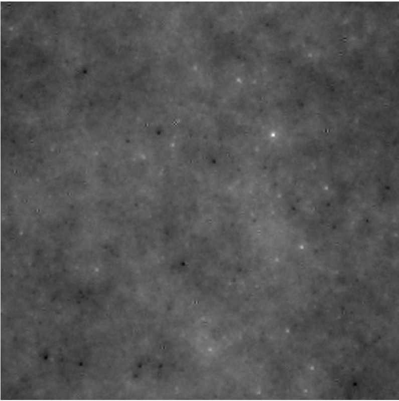 Figure 1
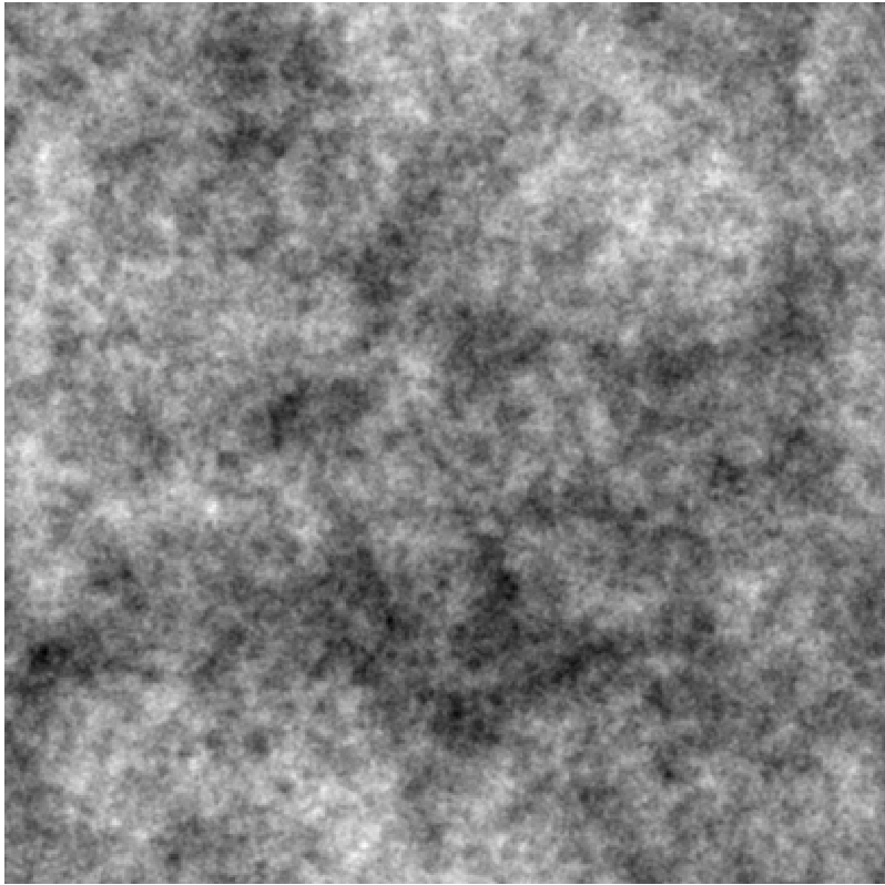 Figure 2
 Figure 3
 Figure 4
Peer Reviews
No public reviews on file for this paper yet. If you reviewed it on a platform where reviews are public (OpenReview, ICLR, NeurIPS, ICML), you can paste yours below so the community can read it here.
Videos
No videos yet. Explain this paper in a talk, walkthrough, or lecture? Add one.
Taxonomy
TopicsAdvanced Harmonic Analysis Research · Mathematical functions and polynomials · Differential Equations and Boundary Problems
Convergence of -Stable Random Fractional Wavelet Series and Some of its Properties
Juan M. Medina, Fernando R. Dobarro and Bruno Cer nuschi-Frías This work was funded by the Universidad de Buenos Aires, Grant. No. 20020170100266BA, CONICET and CONAE, under Project No. 5 of the Anuncio de Oportunidad para el desarrollo de aplicaciones y puesta apunto de metodologías para el área oceanográfica utlizando imágenes SAR, Buenos Aires, Argentina.J. M. Medina and B. Cernuschi-Frías are with the Universidad de Buenos Aires, Facultad de Ingeniería, and the Inst. Argentino de Matemática ”A. P. Calderón”, IAM, CONICET, Buenos Aires, Argentina.F. R. Dobarro is with the Universidad Nacional de Tierra del Fuego, Antártida e Islas del Atlántico Sur, Instituto de Desarrollo Económico e Innovación, Ushuaia, Tierra del Fuego, Antártida e Islas del Atlántico Sur, Argentina.
Abstract
For appropriate orthonormal wavelet basis , constants and , if denotes the Riesz fractional integral operator of order and a sequence of independent identically distributed symmetric -stable random variables, we investigate the convergence of the series . Similar results are also studied for modified fractional integral operators. Finally, some geometric properties related to self similarity are studied.
Index Terms:
Fractional Processes, Wavelets.
I Introduction
Uncoupled representations of random processes are of practical interest. A classical example for Gaussian processes is the Karhunen-Lóeve (KL) representation. Motivated in part by applications in signal and image processing [2, 18, 19, 20], a usual requirement for a random process defined on is to be self similar (see section II-B) in some specified sense, since there exists several related notions in the literature. This property, in the case , is of certain relevance for characterizing textures. For the finite variance case, several KL like representations for the family of of self-similar and related processes were proposed, e.g. [2, 4, 13, 19] among others. In this case, these representations have in general the form:
[TABLE]
where is some fractional integration operator, is an orthonormal basis of or other Hilbert space of functions and the is a sequence of finite variance identically distributed random variables, in most cases Gaussian. The parameter is usually linearly related to the self-similarity Hurst parameter of the process, [3]. Apart from applications, series like (1) and its geometric properties were extensively studied in the case of Fourier Gaussian random series, see for example [9]. Considering this sum as a generalized random process in the sense of Gelfand and Vilenkin [5], Chapter 3, p. 237, if the ’s are Gaussian and is the Riesz fractional integration operator (Definition 3) then this sum converges a.s. in the sense of distributions, i.e. in to a self-similar process as defined here in Section II-B in terms of equality in probability law between and a re-scaled version of it: for some . In this particular case, is a fractional Gaussian noise (See Theorem III.2). These type of representations have received some interest because of its simplicity for modeling certain random signals (see e.g. [19]), since one only needs to know the probability distribution of the coefficients and the parameter or similar. On the other hand, the finite variance requirement may be a constraint in some applications. A first attempt to overcome this limitation, retaining at the same time some of the properties of interest of , is to substitute the ’s with non Gaussian -stable random variables, , [16]. However, it may become a non trivial task to check which properties are preserved for this case. For example, besides self similarity, in [15] is proved that it is not possible to represent a -stable stationary random process by a series like (1).
Here, we prove that for appropriate parameters and , if we consider a suitable wavelet basis, the series (1) stills converges a.s. in , and if we change by a modified operator, then it converges to an ordinary process for the case . If the limit of the series (1) is self similar of parameter , and in the case , although its limit is not necessarily self similar, we can prove that the distribution function of the re-scaled process is, in some sense, properly stochastically dominated. In the Gaussian case of , the series of equation (1) converges to a fractional Gaussian noise, for which an integrated version of it gives the well known fractional Brownian motion, and its -dimensional analogues, with their known “fractal” properties. We shall see that, for appropriate parameters and , that integrated versions of the process have a graph with Hausdorff dimension greater than , justifying the possible use of the process defined by (1) as a model of a fractal process still for .
II Auxiliary results and definitions.
II-A Function spaces, Fourier transforms and Wavelets.
In the following, if and is the Borel measure over , the corresponding Lebesgue spaces of the equivalence classes of functions will be denoted by , and if is the usual Lebesgue measure, we will write shortly . When it becomes a Hilbert space and the inner product will be denoted by . If we will denote its usual norm by and the support of a function is defined by . The Schwartz class of functions is defined as the linear space of smooth functions rapidly decreasing at infinity, together with its derivatives. This means that whenever and
[TABLE]
endowed with its usual topology. We will denote the space of functions which are in and have compact support. Both spaces are topological vector spaces, for more details see [7], Chapter 2, p. 109. Their duals are denoted as: (Tempered distributions) and (distributions) respectively. Clearly: and then . The Fourier Transform of is defined as It is a known fact that also belongs to the space . The Fourier transform can be defined, as usual as a linear map over , as an isometry on or over the class of tempered distributions. The inverse Fourier transform is defined in an analogous way. For further references on Fourier transforms and series, see for example [7].
Below, we will need a variant of the classical Shannon, Nyquist and Kotelnikov sampling theorem.
Theorem** II.1****.**
If is such that with . Then there exists such that
[TABLE]
Proof.
Let be the periodization of . Then, verifies
[TABLE]
and therefore has Fourier series given by
[TABLE]
and then a.e. and in (and in ) norm for a suitable domain . Next, we can take such that
[TABLE]
Defining , then and . This implies
[TABLE]
but (see e.g. [7], Exercise 3.6.4, p.236) , so that
[TABLE]
Then (2) follows immediately from this. ∎
In the following we will use fractional integral operators, for which some of their properties are reviewed. We begin with a definition ([8], Chapter 6, p. 2 or [17], Chapter 5, p. 117):
Definition II.2**.**
Let . For we define its Riesz Potential:
[TABLE]
where .
Riesz potentials have the following scaling property: for every : , i.e. . A crucial result for this integral operator is the following, [8], Chapter 6, p.3 :
Theorem** II.3****.**
*(Hardy, Littlewood and Sobolev) Let , and then:
(a) For all , the integral that defines converges a.e.
(b)If then*
[TABLE]
Note that, in the appropriate sense, the Fourier Transform of is given by:
[TABLE]
and it is easy to check that for and then . Furthermore, if is the Laplacian of , then . Finally, can be thought as defined by the convolution with the locally integrable function , and is formally self adjoint, in the sense that for every :
[TABLE]
Considering again , we can define a fractional integral operator for , in the following way:
[TABLE]
The modified kernel is easier to control, and we sketch the proof of the following lemma:
Lemma** II.4****.**
*If and , then and moreover:
(i) There exists a positive constant such that for each :*
[TABLE]
(ii) For every : .
Proof.
(Sketch) Since
[TABLE]
The condition gives the appropriate exponent for the boundedness of the first integral. In addition, since and considering that for some positive constant
[TABLE]
if , then the second integral is also finite. Hence, the map is well defined and by a change of variable, we obtain that it is an homogeneous function depending only on , from which assertion (i) follows. Assertion (ii) is also obtained by a change of variable. ∎
For fixed , we note that in the Fourier domain can be characterized, in an appropriate sense, [2], Chapter 3, p. 45, by:
[TABLE]
Some formal manipulations show that from equations (5) and (7), for suitable parameters and , we have:
[TABLE]
and
[TABLE]
For another related operator is defined, formally, by its Fourier transform as:
[TABLE]
Theorem** II.5****.**
[8]**, Chapter 6, p. 8. If and , defines a continuous linear operator, i.e. there exists such that
[TABLE]
For , and , we introduce the Sobolev spaces :
[TABLE]
These are Banach spaces of tempered distributions with the norm defined by . Moreover, [14], p.168, if , this norm is equivalent to . Recalling again equation (7) the equivalence of norms for takes the following form which will be useful in the sequel:
[TABLE]
In the particular case , only when , the spaces coincide with the following spaces, which are introduced for auxiliary purposes.
Proposition** II.6****.**
For , the space
[TABLE]
is a Banach space with the norm defined by . Moreover convergence in implies convergence in .
Proof.
Observe that if we define , then if and only if . Let be a Cauchy sequence en which is equivalent to being a Cauchy sequence in , and then there exists a unique such that , when . We shall verify that and therefore taking we are done. For this take and then by Hölder’s inequality:
[TABLE]
[TABLE]
thus, see e.g. [7], Exercise 2.3.1, p.122, and therefore . Finally, in if and only if in . Let , then, if , by definition of the Fourier Transform of a tempered distribution and Hölder’s inequality we get:
[TABLE]
[TABLE]
[TABLE]
which proves the last assertion of Proposition II.6. ∎
The following estimate for the norm will be useful in the sequel.
Lemma** II.7****.**
Let , then and moreover, if , there exits a positive constant such that for every , a.e. in , the following inequality holds:
[TABLE]
Proof.
If the result is immediate. To prove the first assertion for , by Hölder’s inequality one has the following estimate
[TABLE]
For the second assertion, under these conditions we can write
[TABLE]
as in Theorem II.1 and therefore:
[TABLE]
[TABLE]
[TABLE]
since by Peetre’s inequality. If , take and
[TABLE]
by Hölder’s inequality we get:
[TABLE]
finally, since there exists some positive constant such that:
[TABLE]
then equation (14) becomes
[TABLE]
[TABLE]
∎
II-B Some probability, stable laws and generalized random processes.
Let be a probability space and a random variable variable defined on it. The distribution function of is defined, for , as . If is any Borel measurable real function, we will denote the expectation of with . The characteristic function of is . For , we say that a random variable is symmetric -stable of parameter if . A symmetric -stable random variable will be denoted as . When we write we shall be referring to the distribution function of such a random variable with . Note that corresponds to the Gaussian case and therefore . Let us review some basic properties of stable distributions, see [16], Chapter 1, p. 10, and [10], Chapter 0, p.5.
If are independent and , with parameter then , with . 2. 2.
Let . If and then , where , and for .
Let be a non negative Borel measure on . We shall need a result on the a.s. convergence of random elements in . This theorem is a particular case of a more general one in [10], Chapter 2.
Theorem** II.8****.**
Let , , and let be a sequence of independent and identically distributed random variables. Then the series converges in a.s. if and only if
[TABLE]
Our results, are aimed at the construction of certain random variables taking values in . In this case, every - valued random variable, say , takes the form of a random linear functional defined on . Previously, we will also need to define the class of generalized random processes, of which these - valued random variables are particular cases. Following [5], Chapter 3, p. 237, and [19], Chapter 4, p. 57, we will say that a generalized random functional is defined on if for every there is associated a real valued random variable . In accordance with the usual specification of the probability distributions of a countable set of real random variables, given , define the probability of the events, which will have to be compatible in the usual sense. On the other hand, linearity means that for any , : . For a comprehensive study on this topic, see [5]. In an analogous way to real valued random variables, for each we can calculate the characteristic function of the real random variable , . In fact if and considering as a variable, this gives the characteristic functional of , , which completely determines its distributions as in the case of ordinary random processes. Finally, self-similarity for generalized random processes can be defined in the following analogous way to [19], p. 178: is self-similar if there exists a constant such that
[TABLE]
for every dilation factor and . This means that is equivalent, in probability law, to , for some appropriate constant . In this context, we recall the Hausdorff dimension, see [3], Chapter 2, p. 21, of a subset of denoted by . Although self similarity is associated to the notion of “fractality”, the last one has not a precise meaning. However, subsets of with non integer Hausdorff dimension are considered as displaying a fractal behaviour. A way for the study of the fractal behaviour of the graph of a function is the calculation of its Hausdorff dimension. Usually, the estimation of a lower bound for this value is calculated by potential methods, see [3], Chapter 2, p. 26, and [9], Chapter 10, p.132. An example is:
Lemma** II.9****.**
If is a compact subset of and denotes the graph of a measurable function and then .
Other related results will be introduced in the final section, for the estimation of the Hausdorff dimension of certain processes arising from the construction introduced in equation (1).
II-C Wavelets.
Let , with , be an orthonormal wavelet basis of , [14], Chapter 2. The Parseval identity for this case is:
[TABLE]
Therefore the norm can be estimated from the wavelet coefficients . Under some additional conditions, for example if the wavelet basis arises from a -regular wavelet multirresolution approximation of , then, if denotes the family of dyadic cubes of , for some positive constants , we have the following estimations for the and norms respectively, [14], Chapter 6:
[TABLE]
and for ,
[TABLE]
In order to simplify the notation involving wavelet expansions we will sometimes omit the summation limits as in equations (17) and (18).
III Main Results.
III-A Convergence.
First, we prove an inequality involving the norm of the wavelet coefficients of a function. As a byproduct, this inequality implies one case of the Sobolev’s embeddings, see e.g. [1], Theorem 7.57.
Theorem** III.1****.**
Let be an -regular orthonormal wavelet basis, and then there exists a positive constant such that:
[TABLE]
for all . If , the inequality (19) holds for .
Proof.
The case is immediate since . If , the lower bound holds, since
[TABLE]
The upper bound is obtained splitting the sum:
[TABLE]
Then for each :
[TABLE]
since for fixed , if . The inner integrand can be rewritten as
[TABLE]
[TABLE]
by Hölder’s inequality with exponents and and since . Hence
[TABLE]
[TABLE]
For the bound on the other term, we proceed similarly to the previous case:
[TABLE]
Therefore by by Hölder’s inequality with exponents and , if
[TABLE]
we get
[TABLE]
[TABLE]
Combining equations (20) and (21) and since is finite we get the result. ∎
Now, we can prove one of the main results of this work.
Theorem** III.2****.**
Let be an -regular orthonormal wavelet series, with , , and a sequence of independent identically distributed random variables such that . Then the series defined by
[TABLE]
converges a.s. in . If , the result remains true for .
Proof.
We shall prove the case , the case is very similar using Parseval’s identity instead of Theorem III.1. Let , since , then by lemma II.7,
[TABLE]
thus
[TABLE]
[TABLE]
But, if , a density argument applied to equation (6) gives:
[TABLE]
Therefore, by Theorem III.1, and taking :
[TABLE]
[TABLE]
The last inequality holds by the Hardy-Littlewood and Sobolev Inequality with exponents . Note that the validity of this last step is granted since and . Moreover is finite and constant in . Thus from the definition of combined with equations (24), (23) and (22):
[TABLE]
[TABLE]
Taking any , by Hölder’s inequality combined with equation (25):
[TABLE]
[TABLE]
then, by Theorem II.8,
[TABLE]
converges a.s. in and therefore converges a.s. in and in . With slight modifications, the same argument works with any translate of . Finally, to verify that converges a.s. in , take , with defined by
[TABLE]
and . For fixed , and we have
[TABLE]
and then
[TABLE]
for some such that since has compact support. The result follows from the convergence of when for each . ∎
Alternatively, considering and the operators instead of we can prove:
Theorem** III.3****.**
Let be an -regular orthonormal wavelet series, , , and a sequence of independent identically distributed random variables such that . Then, for each the series defined by
[TABLE]
converges almost surely. Moreover, has a measurable version. If , the result remains true for .
Remark.
Note that the range of validity of the result depends on the dimension , since the restrictions imply that for .
Proof.
Recall the properties of the stable random variables reviewed in Section II-B. For each , we can prove the convergence in -mean () of the sum defining . By Theorem III.1, and taking any such that , since for some constant . we obtain:
[TABLE]
since, recalling from Section II-A the Lemma II.4, and the equivalence of norms of given by equation (11), one obtains:
[TABLE]
[TABLE]
The sum defining converges a.s. since convergence in the -mean of independent random variables implies a.s. convergence. Similarly to the previous bound, if , by Lemma II.4 (ii) one gets:
[TABLE]
[TABLE]
[TABLE]
From this, applying Tchebychev’s inequality, it follows the stochastic continuity of , and then there exists a measurable version (Theorem 1, p.157 of [6]) of . ∎
III-B Self similarity analysis
Self similarity in the sense of equation (15) is broken if . However, the following results show that, in some sense, the rescaled versions of are stochastically dominated. Furthermore, we may expect some kind of fractal behavior for an integrated version of , as the realizations of considering a Daubechies wavelet basis suggest, see Figures 1 and 2.
Theorem** III.4****.**
Under the same hypothesis of Theorem III.2, the generalized random process defined by:
[TABLE]
is self similar if , in the sense that for every , has the same distribution function as , and otherwise, for every , there exists a positive constant such that the following bounds hold:
[TABLE]
[TABLE]
for every , and .
Remark
Note that in the case it is easy to verify that the limit process is a Gaussian fractional noise with characteristic functional , and that this stationary generalized random process has a spectral measure, [5], Chapter 3, given by . However, if , the analogous result for the stable case does not hold, since , which corresponds to the case of fractional stable noise.
Proof.
Let and . To prove equation (27) it is sufficient to analyze , the characteristic function of the real random variable . From the scaling property of :
[TABLE]
Assume with no loss of generality. Since the ’s are independent and identically distributed with characteristic function , then the sum defining has characteristic function given by:
[TABLE]
which corresponds to the distribution
[TABLE]
Then, the upper bound follows combining Theorem III.1 and the fact that is monotone. The lower bound is obtained similarly estimating the norm
[TABLE]
Finally, the case is obtained in an analogous way with equality due to Parseval’s identity for the orthonormal basis of . ∎
The previous result is a consequence of the bound derived from Theorem III.1:
[TABLE]
For , and taking a sequence such that in as , provided that are as in Theorem III.3, we can interpret as an integrated observation of : , where these equalities are only formal. In fact is a well defined ordinary random variable for each . Recalling equation (8) and Section II-B, its characteristic function is given by
[TABLE]
which is the pointwise limit of the sequence of characteristic functions
[TABLE]
This is a consequence of the following bound, which again can be derived from Theorem III.1 with :
[TABLE]
[TABLE]
[TABLE]
The Lebesgue measure in of a measurable version of is zero. Let us bound, from below, the Hausdorff dimension of the graph of . As a consequence, we shall see that for suitable parameters, the Hausdorff dimension has non integer values.
Theorem** III.5****.**
Under the same hypothesis of Theorem III.3, then a.s., where is the graph of .
Proof.
The lower bound is a consequence of Lemma II.9. We shall prove that
[TABLE]
if . Let us write , then recalling equation (29), by Lemma II.4, (i) and (ii), one gets:
[TABLE]
[TABLE]
Hence, from equation (30) :
[TABLE]
[TABLE]
and therefore, if for example without loss of generality ,
[TABLE]
[TABLE]
provided that , which concludes the proof. ∎
Acknowledgment.
The authors thank the collaboration of Alexandre Chevallier, visiting student from the École Internationale des Sciences du Traîtement de l’Information, École d’Ingénieurs Mathématiques, for the computer simulations corresponding to Figures 1 and 2.
The reference list from the paper itself. Each links out to its DOI / PubMed record.
- 1[1] Adams R.A., Sobolev Spaces , Academic Press, 1975.
- 2[2] Cohen S., Istas J., Fractional Fields and Applications , Springer, 2013.
- 3[3] Falconer K., Techniques in fractal geometry , Wiley, 1997.
- 4[4] Flandrin P., “Wavelet analysis and synthesis of fractional Brownian motion”, IEEE Trans. Inf. Theory . IT 38(2), pp. 910-917, 1992.
- 5[5] Gel’fand I.M. Vilenkin N. Ya. Generalized Functions . Vol. IV. Fizmatgiz, Moscow, 1961.(Russian). English trnsl. Academic Press, New York, 1964.
- 6[6] Gikhman I.I., Skorokhod A.V. Introduction to the theory of random processes , Dover, 1996.
- 7[7] Grafakos L. Classical Fourier Analysis . Vol.I, GTM 249, Second Edition, Springer, 2008.
- 8[8] Grafakos L. Modern Fourier Analysis . Vol.I, GTM 250, Second Edition, Springer, 2008.