TL;DR
This paper introduces a new influence measure based on information geometry to quantify the sensitivity of deep neural networks to various perturbations, aiding in understanding model robustness and vulnerability.
Contribution
It proposes a novel perturbation manifold and influence measure that are invariant and applicable to multiple model analysis tasks in DNNs.
Findings
Effective in detecting outliers and vulnerable areas.
Useful for comparing sensitivity across models and datasets.
Demonstrated on ResNet50 and DenseNet121 with CIFAR10 and MNIST.
Abstract
Deep neural networks (DNNs) have achieved superior performance in various prediction tasks, but can be very vulnerable to adversarial examples or perturbations. Therefore, it is crucial to measure the sensitivity of DNNs to various forms of perturbations in real applications. We introduce a novel perturbation manifold and its associated influence measure to quantify the effects of various perturbations on DNN classifiers. Such perturbations include various external and internal perturbations to input samples and network parameters. The proposed measure is motivated by information geometry and provides desirable invariance properties. We demonstrate that our influence measure is useful for four model building tasks: detecting potential 'outliers', analyzing the sensitivity of model architectures, comparing network sensitivity between training and test sets, and locating vulnerable areas.…
Click any figure to enlarge with its caption.
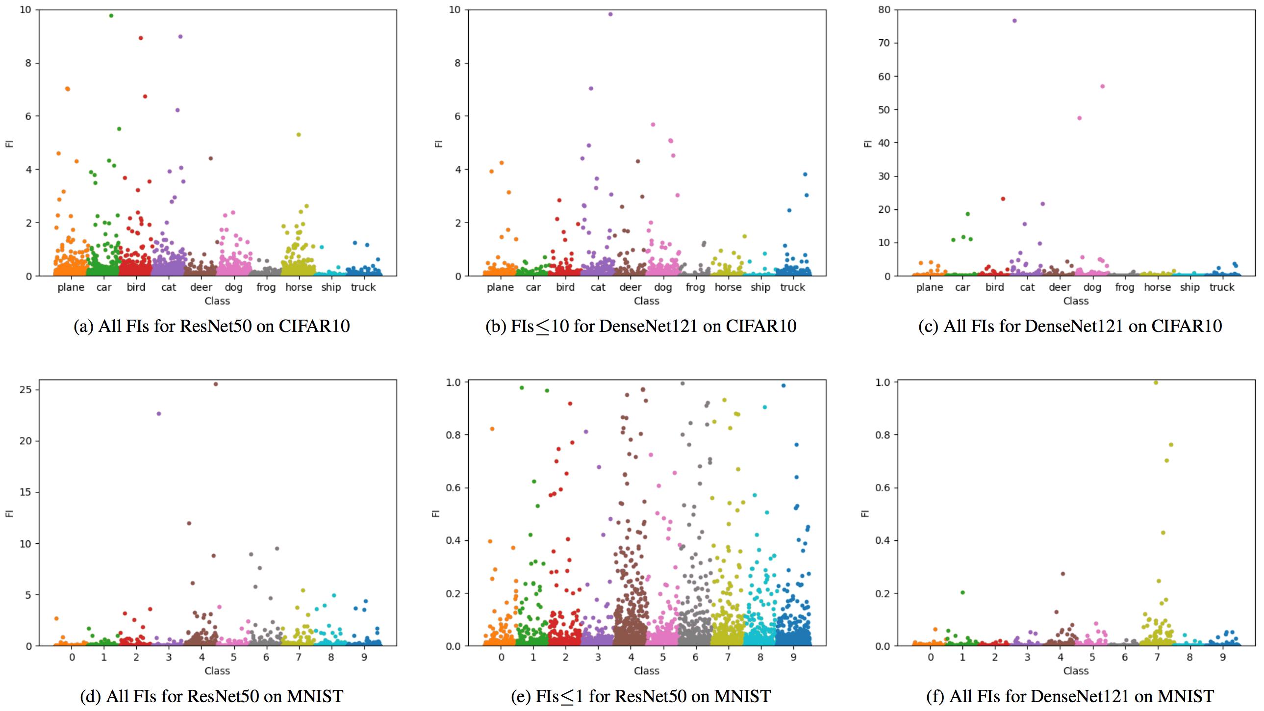 Figure 1
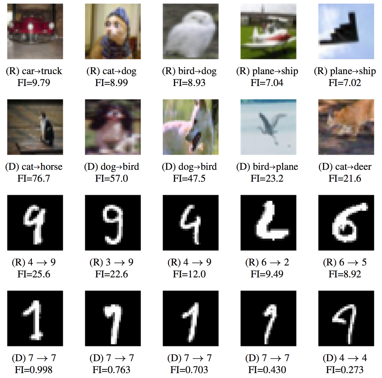 Figure 2
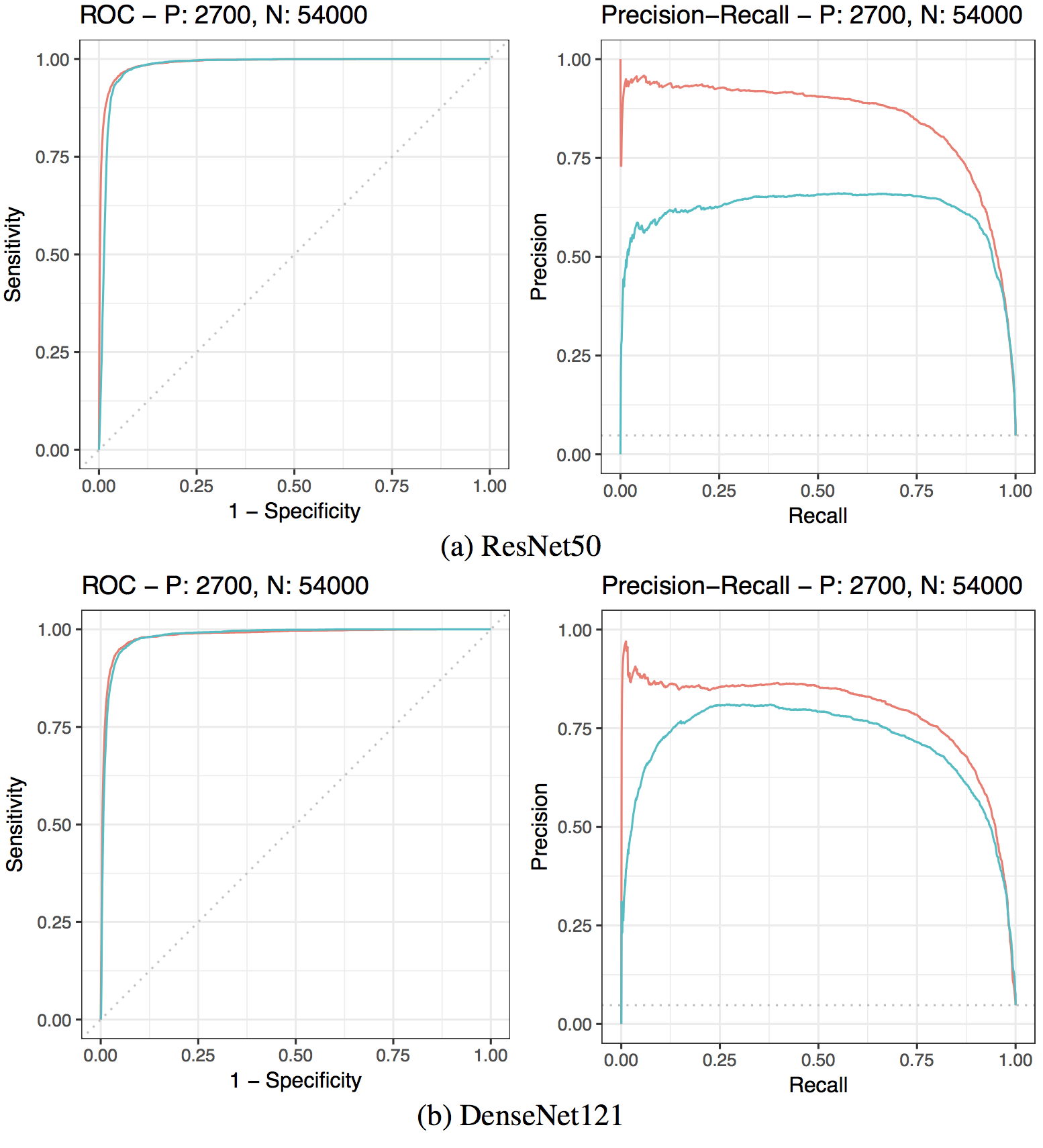 Figure 3
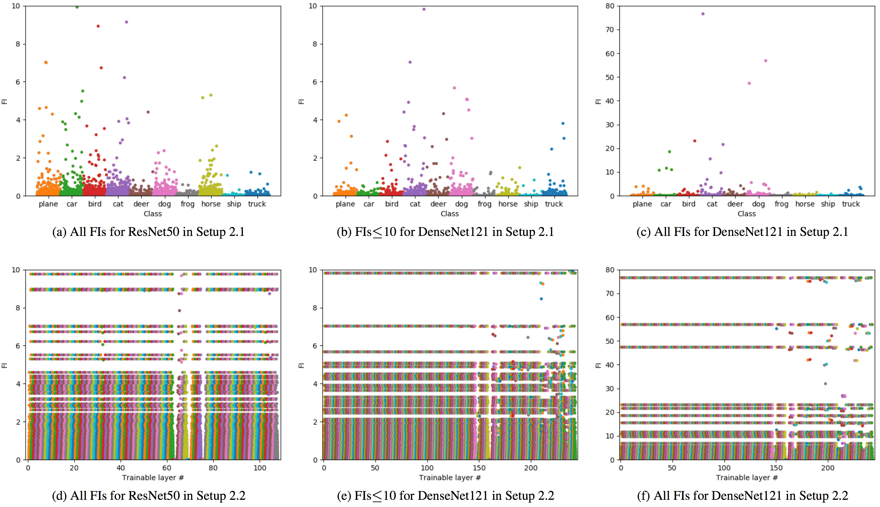 Figure 4
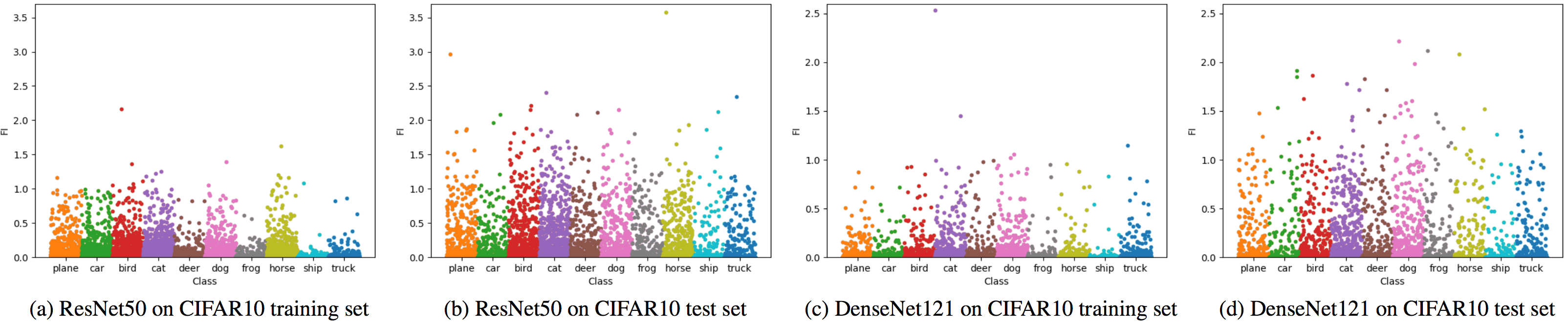 Figure 5
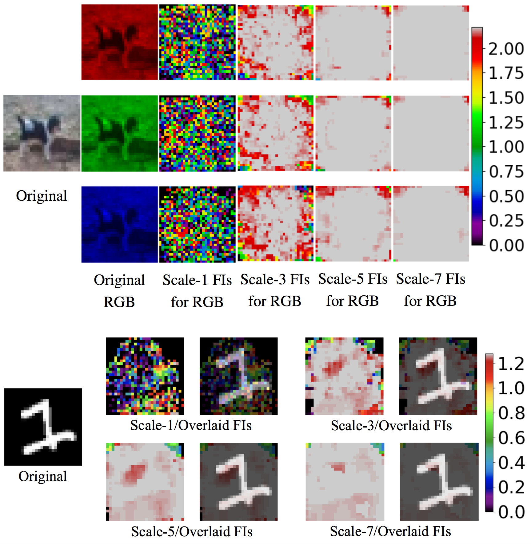 Figure 6
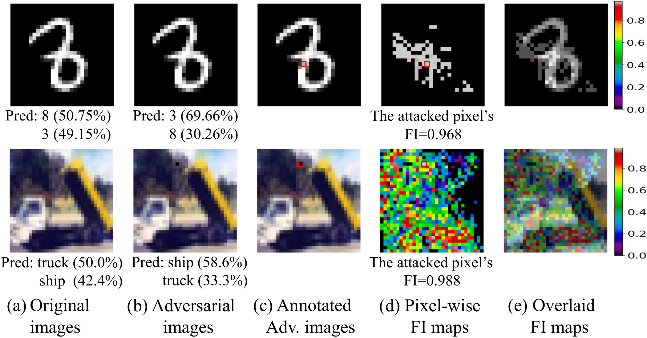 Figure 7
| CIFAR10 | MNIST | ||||
|---|---|---|---|---|---|
| Model | Training | Test | Training | Test | |
| ResNet50 | 99.78% | 88.70% | 99.87% | 99.29% | |
| DenseNet121 | 99.87% | 91.16% | 99.998% | 99.58% | |
| ResNet50 | DenseNet121 | ||||
|---|---|---|---|---|---|
| Percentile | Training | Test | Training | Test | |
| 75th | 2.87e-3 | 0.031 | 1.10e-4 | 1.83e-3 | |
| 80th | 5.38e-3 | 0.073 | 2.42e-4 | 6.57e-3 | |
| 85th | 0.010 | 0.160 | 6.00e-4 | 0.025 | |
| 90th | 0.023 | 0.343 | 1.78e-3 | 0.097 | |
| 95th | 0.064 | 0.678 | 7.80e-3 | 0.352 | |
| 98th | 0.177 | 0.999 | 0.037 | 0.755 | |
| 99th | 0.316 | 1.215 | 0.099 | 0.951 | |
| 100th | 2.160 | 3.579 | 2.533 | 2.215 | |
Peer Reviews
No public reviews on file for this paper yet. If you reviewed it on a platform where reviews are public (OpenReview, ICLR, NeurIPS, ICML), you can paste yours below so the community can read it here.
Code & Models
Videos
No videos yet. Explain this paper in a talk, walkthrough, or lecture? Add one.
Sensitivity Analysis of Deep Neural Networks
Hai Shu
Department of Biostatistics
The University of Texas MD Anderson Cancer Center
Houston, Texas, USA &Hongtu Zhu
AI Labs, Didi Chuxing
Beijing, China
Abstract
Deep neural networks (DNNs) have achieved superior performance in various prediction tasks, but can be very vulnerable to adversarial examples or perturbations. Therefore, it is crucial to measure the sensitivity of DNNs to various forms of perturbations in real applications. We introduce a novel perturbation manifold and its associated influence measure to quantify the effects of various perturbations on DNN classifiers. Such perturbations include various external and internal perturbations to input samples and network parameters. The proposed measure is motivated by information geometry and provides desirable invariance properties. We demonstrate that our influence measure is useful for four model building tasks: detecting potential ‘outliers’, analyzing the sensitivity of model architectures, comparing network sensitivity between training and test sets, and locating vulnerable areas. Experiments show reasonably good performance of the proposed measure for the popular DNN models ResNet50 and DenseNet121 on CIFAR10 and MNIST datasets.
1 Introduction
Deep neural networks (DNNs) have exhibited impressive power in image classification and outperformed human detection in the ImageNet challenge (?; ?; ?; ?). Despite this huge success, it is well known that state-of-the-art DNNs can be sensitive to small perturbations (?; ?; ?; ?; ?). This vulnerability has called into question their usage in safety-critical applications, including self-driving cars (?) and face recognition (?), among many others (?). There is rich literature on quantifying the sensitivity or robustness of DNNs to external perturbations that affect the input samples; see (?; ?; ?). For instance, one popular robustness measure computes the minimum adversarial distortion for a given sample (?; ?; ?). However, very little work has been done on measuring the effects of various internal perturbations to network trainable parameters on DNNs. To the best of our knowledge, (?) is the first paper to examine the robustness of AlexNet (?) by tracking the classification performance over several chosen standard deviations of Gaussian perturbations to network weights.
The aim of this paper is to develop a novel perturbation manifold and its associated influence measure to evalute the effects of various perturbations to input samples and/or network trainable parameters. Our influence measure is a novel extension of the local influence measures proposed in (?; ?) to classification problems by using information geometry (?; ?). Compared with the existing methods (?), we make the following two major methodological contributions.
Our influence measure is motivated by information geometry, and its calculation is computationally straightforward and does not require optimizing any objective function. When the dimension of the perturbation vector is larger than the number of classes, the perturbation manifold in (?; ?) has a singular metric tensor and thus fails to form a Riemannian manifold. We address this singularity issue by introducing a low-dimensional transform and show that our influence measure still provides the invariance under diffeomorphisms of the original perturbation. Such an invariance property is critical for assessing the simultaneous effects or comparing the individual impacts of different external and/or internal perturbations within or between DNNs without concerning their difference in scales, such as the comparison between perturbations to trainable parameters in a convolution layer and those in a batch normalization layer within a single DNN. In contrast, existing measures, such as the Jacobian norm (?) and Cook’s local influence measure (?), do not have this invariance property, leading to some misleading results.
Our proposed influence measure is applicable to various forms of external and internal perturbations and useful for four important model building tasks: (i) detecting potential ‘outliers’, (ii) analyzing the sensitivity of model architectures, (iii) comparing network sensitivity between training and test sets, and (iv) locating vulnerable areas. For task (i), downweighting outliers may be used to train a DNN with increased robustness. Task (ii) may serve as a guide to the improvement of an existing network architecture. Task (iii) can evaluate the heterogeneity of the model robustness between training and test sets, and combining tasks (i)–(iii) may be useful for selecting DNNs. For task (iv), the discovered vulnerable locations in a given image can be utilized to either craft adversarial examples or fortify a DNN with data augmentation. The application of our influence measure to tasks (i)-(iv) is illustrated for two popular DNNs, ResNet50 (?) and DenseNet121 (?), on the benchmark datasets CIFAR10 and MNIST.
2 Method
2.1 Perturbation Manifold
Given an input image and a DNN model with a trainable parameter vector , the prediction probability for the response variable is denoted as Let be a perturbation vector varying in an open subset . The perturbation can be flexibly imposed on , , or even the combination of and . Denote to be the prediction probability under perturbation such that . It is assumed that there is a such that . Also, is assumed to be positive and sufficiently smooth for all .
Following the development in (?; ?), we may define as a perturbation manifold. The tangent space of at is denoted by , which is spanned by , where . Let with . If is positive definite, then for any two tangent vectors , , where denotes the coordinate vector of on the basis , the inner product can be defined by
[TABLE]
Subsequently, the length of is given by
[TABLE]
With the above inner product defined by , is a Riemannian manifold and is the Riemannian metric tensor (?; ?).
We need the positive definiteness of . However, as a sum of rank-1 matrices has , so it is a singular matrix when . The case is true in many classification problems since the number of classes is often much smaller than the dimension of . The singularity of indicates that the tangent vectors are linearly dependent and thus some components of are redundant. In addition, our focus is on the small perturbations around . We hence transform the -dimensional to be a vector such that is positive definite in a small neighborhood of that corresponds to .
Our low-dimensional transform is implemented as follows. We first obtain a compact singular value decomposition (cSVD) of . For very large , rather than the direct but extremely expensive cSVD computation of the matrix, we apply a computationally efficient approach using the cSVD of the much smaller matrix by noticing that . Let . The usual cSVD computation can easily yield that and , where is a matrix with orthonormal columns, is a orthogonal matrix and is a diagonal matrix. We hence obtain the cSVD: with . Define the desirable transform of by . Denote , where and . It follows from that . By the smoothness of in , the metric tensor is positive definite in an open ball centered at .
Definition 1**.**
We define the Riemannian manifold with the inner product defined by in (2.1) as the perturbation manifold around .
2.2 Influence Measure
Let be the objective function of interest for sensitivity analysis. We define the influence measure to evaluate the discrepancy of the objective function at two points, and , corresponding to , on the perturbation manifold . Let be a smooth curve on connecting to , where with a smooth curve connecting to . The distance between and along the curve is defined by
[TABLE]
with . Following (?), the influence measure for along is given by
[TABLE]
Let , then . We define the (first-order) local influence measure of at by
[TABLE]
Denote , , , , and \mathbf{H}_{f(\boldsymbol{\omega}_{0})}=\frac{\partial^{2}f}{\partial\boldsymbol{\omega}\partial\boldsymbol{\omega}^{T}}\big{|}_{\boldsymbol{\boldsymbol{\omega}}=\boldsymbol{\omega}_{0}}. Plugging and into (2) yields the closed form
[TABLE]
where , is the pseudoinverse of , and we used the identities and
Definition 2**.**
We define the influence measure of at by given in (2) with the closed form in (2.2).
Theorem 1**.**
Suppose that is a diffeomorphism of . Then, is invariant with respect to any reparameterization corresponding to .
Proof.
Let , , and . Denote their Jacobian matrices by and . Differentiating with respect to yields . Denote , , and . We have
[TABLE]
∎
Theorem 1 shows the invariance of under any diffeomorphic (e.g., scaling) reparameterization of the original perturbation vector rather than . This result is analogous to those in (?; ?), but we extend it to cases where the original perturbation model with is not a Riemannian manifold, especially when .
The invariance property is not enjoyed by the widely used Jacobian norm (?) and Cook’s local influence measure (?). For example, consider the perturbation , where is a subvector of , and the scaling version with . Let and its scaling counterpart . We have that the Jacobian norm
[TABLE]
and the Cook’s local influence measure
[TABLE]
with are not scaling-invariant. This is problematic especially when the scale heterogeneity exists between parameters to which the perturbations are imposed. For instance, in the simultaneous perturbations to both input image and trainable network parameters , i.e., , the contribution of appears to be exaggerated if is scaled with larger values than . Another example is the comparison between perturbations to trainable parameters (weights and bias) in a convolution layer and those (shift/scale parameters) in a batch normalization layer. There are no uniform criteria for the scaling because either rescaling to a unit norm or keeping on the original scales seems to have its own advantages. However, our influence measure evades this scaling issue by utilizing the metric tensor of the perturbation manifold rather than that of the usual Euclidean space.
2.3 Perturbation Examples
In this subsection, we illustrate how to compute the proposed influence measure for a trained DNN model . We consider the following commonly used perturbations to the input image or the trainable parameters , where are the parameters in the -th trainable network layer.
- •
Case 1: ;
- •
Case 2: ;
- •
Case 3: .
All three cases can be written in a unified form with . Let the perturbation vector and . For the influence measure in (2.2), we have
[TABLE]
where and are obtained starting from matrix through , and . The component in is now computed by
[TABLE]
The gradients and can be calculated easily via backpropagation (?) in deep learning libraries like TensorFlow (?) and Pytorch (?).
Next, we consider a specific DNN example under Case 3. Consider the following feedforward DNN architecture before the softmax layer:
[TABLE]
where , , , and ’s are entry-wise activation functions. For notational simplicity, we set all bias terms to zero and consider the sigmoid function
[TABLE]
for all activation functions. Let and be the input and output vectors of the -th layer such that and . The softmax function is given by
[TABLE]
The whole DNN model is
[TABLE]
for , where is the -th entry of vector . Under Case 3, we have . Choose the objective function to be the cross-entropy, i.e.,
[TABLE]
Hence, in (6) we have . Then, to calculate the gradients in (6) and (7), we only need to consider Note that where has 1 in the -th entry and 0 in the others. Moreover, with and Hence, for (6) and (7), we have
[TABLE]
3 Experiments
In this section, we investigate the performance of our local influence measure. We address the four tasks stated in Introduction through the following setups under the three perturbation cases in Section 2.3.
- •
Setup 1: Compute each training image’s FI under Case 1, with being the cross entropy, i.e., .
- •
Setup 2: Let .
- –
Setup 2.1: Compute each training image’s FI under Case 2.
- –
Setup 2.2: Compute each trainable network layer’s FI under Case 3 for each training image.
- •
Setup 3: Compute each image’s FI under Case 1 for both training and test sets, where .
- •
Setup 4: Compute each pixel’s FI under Case 1 for a given image. We adopt a multi-scale strategy taking into account the spatial effect. For each pixel, we set in Case 1 to be the square centered at the pixel with the scale . We use .
For the cross-entropy like function in Setups 3 and 4, we use the predicted label instead of the true label for the prediction purpose rather than the training purpose in the first two setups. In Setup 4, the scale of the pixel-level FI is analogous to the convolutional kernel size.
We conduct experiments on the two benchmark datasets CIFAR10 and MNIST using the two popular DNN models ResNet50 (?) and DenseNet121 (?). Originally, there are 50,000 and 60,000 training images for CIFAR10 and MNIST, respectively. As the validation sets, we use randomly selected 10% of those images, with the same number for each class. No data augmentation is used for the training process. Both datasets have 10,000 test images. The prediction accuracy of our trained models is summarized in Table 1.
3.1 Outlier Detection
We study the outlier detection ability of our proposed influence measure under Setup 1. Figure 1 illustrates the results of Setup 1 by using Manhattan plots. DenseNet121 generally has smaller FIs than ResNet50 for the two benchmark datasets, excluding several large FIs over 10 shown in Figure 1(c) for CIFAR10. The images with the top 5 largest FIs are displayed in Figure 2 for each case. Most of the 20 images, especially those in MNIST, are difficult even for human visual detection. This indicates the strong power of our influence measure in detecting outlier images.
We further examine the outlier detection power of our proposed influence measure by simulating outlier images from MNIST. Each outlier image was generated by overlapping two training digits of different classes that are shifted up to 4 pixels in each direction, with the true label randomly set to be one of the two classes. The two DNN models in Table 1 are trained with additional 50 epochs after incorporating 2700 and 300 simulated outlier images into the training and validation sets, with accuracies reduced up to 0.38% and 0.11% for respective training and testing. The original 54,000 training images are all treated as non-outliers. We compare the proposed FI measure with the Jacobian norm given in (4) using the cross-entropy as the objective function . The maximal Cook’s local influence, , is not considered here due to the expensive computation of the very large Hessian matrix; see (2.2). Figure 7 shows the outlier detection results of the two considered measures. Although the receiver operating characteristic (ROC) curves of the two measures are almost overlapping, our FI measure significantly outperforms Jacobian norm in terms of the precision-recall (PR) curves that are more useful for highly unbalanced data (?).
3.2 Sensitivity Analysis on DNN Architectures
We conduct the sensitivity analysis on DNN architectures under Setup 2. The invariance property of our FI measure shown in Theorem 1 enables us to fairly compare the effects of small perturbations to model parameters of different scales within or between DNNs. Setup 2.1 compares the sensitivity between the two DNNs, while Setup 2.2 undertakes the comparison across trainable layers within each single DNN.
The Manhattan plots for Setup 2 on CIFAR10 are presented in Figure 4; results for MNIST are provided in the Supplementary Material. The patterns on CIFAR10 under Setup 2.1 in Figure 4(a)-(c), with mostly smaller FIs for DensetNet121, are quite similar to those for Setup 1 in Figure 1(a)-(c), indicating that DenseNet121 is generally less sensitive than ResNet50 to the infinitesimal perturbations to all network trainable parameters. From Figure 4(d)-(f) for Setup 2.2, we see stable patterns of FIs over the trainable layers for the two DNNs. Modifying their network architectures does not appear to be necessary here. Note that the FI value for the trainable parameters in each single network layer is theoretically dominated by that for all trainable parameters of the entire network, which is well supported by the comparison between Figure 4(a)-(c) and (d)-(f).
3.3 Sensitivity Comparison between Training and Test Sets
We compare the network sensitivity between training and test sets under Setup 3. Figure 5 and Table 2 show the FI values for Setup 3 on CIFAR10; results for MNIST are also provided in the Supplementary Material. In the figure and table, the test set has more slightly large FIs than the training set for both DNNs, while FIs are generally smaller in both sets for DenseNet121. We suggest to select a DNN model with similar sensitivity performance and smaller FI values on both training and test sets. Together with the results of Sections 3.1 and 3.2 shown in Figure 1 (a)-(c) and Figure 4 (a)-(c), and also with the model accuracies in Table 1, DenseNet121 is preferred over ResNet50 on CIFAR10 in terms of both sensitivity and accuracy.
3.4 Vulnerable Region Detection
We apply the multi-scale strategy in Setup 4 to detect the areas in an image that are vulnerable to small perturbations.
For Setup 4, the test images from the two benchmark datasets with the largest FI in Setup 3 by DenseNet121 are illustrated in Figure 6. The vulnerable areas for both images are mainly in or around the object, and the image boundaries are generally less sensitive to perturbations. The figure also reasonably shows that the vulnerable areas expand as the scale of pixel-level FI increases.
Figure 7 illustrates the one-pixel adversarial attacks based on pixel-wise FI maps. The two selected test images are correctly predicted by ResNet50 with a high probability and also with a large FI in Setup 3. The pixel-wise FI map denotes the scale-1 pixel-level FI map for the MNIST image, and is the average scale-1 map over the three RGB channels for the CIFAR10 image. For each image, the attacked pixel is the one with the largest value in the pixel-wise FI map. We see that the prediction result significantly changes after slightly altering the selected pixel’s value. This indicates that our FI measure is useful for discovering vulnerable locations and crafting adversarial examples.
4 Conclusion
In this paper, we introduced a novel perturbation manifold and its associated influence measure for sensitivity analysis of DNN classifiers. This new measure is constructed from a Riemannian manifold and provides the invariance property under any diffeomorphic (e.g., scaling) reparameterization of perturbations. This invariance property is not owned by the widely used measures like the Jacobian norm and Cook’s local influence. Our influence measure performs very well for ResNet50 and DenseNet121 trained on CIFAR10 and MNIST datasets in the tasks of outlier detection, sensitivity comparison between network architectures and that between training and test sets, and vulnerable region detection.
The reference list from the paper itself. Each links out to its DOI / PubMed record.
- 1[Abadi et al . 2016] Abadi, M.; Barham, P.; Chen, J.; Chen, Z.; Davis, A.; Dean, J.; Devin, M.; Ghemawat, S.; Irving, G.; Isard, M.; Kudlur, M.; Levenberg, J.; Monga, R.; Moore, S.; Murray, D. G.; Steiner, B.; Tucker, P.; Vasudevan, V.; Warden, P.; Wicke, M.; Yu, Y.; and Zheng, X. 2016. Tensorflow: A system for large-scale machine learning. In 12th USENIX Symposium on Operating Systems Design and Implementation (OSDI 16) , 265–283.
- 2[Akhtar and Mian 2018] Akhtar, N., and Mian, A. 2018. Threat of adversarial attacks on deep learning in computer vision: A survey. ar Xiv preprint ar Xiv:1801.00553.
- 3[Amari and Nagaoka 2000] Amari, S., and Nagaoka, H. 2000. Methods of Information Geometry . American Mathematical Society, Providence, RI.
- 4[Amari 1985] Amari, S. 1985. Differential-geometrical Methods in Statistics . Springer-Verlag, New York.
- 5[Bojarski et al . 2016] Bojarski, M.; Del Testa, D.; Dworakowski, D.; Firner, B.; Flepp, B.; Goyal, P.; Jackel, L. D.; Monfort, M.; Muller, U.; Zhang, J.; et al. 2016. End to end learning for self-driving cars. ar Xiv preprint ar Xiv:1604.07316.
- 6[Carlini and Wagner 2017] Carlini, N., and Wagner, D. 2017. Towards evaluating the robustness of neural networks. In 2017 IEEE Symposium on Security and Privacy , 39–57.
- 7[Cheney, Schrimpf, and Kreiman 2017] Cheney, N.; Schrimpf, M.; and Kreiman, G. 2017. On the robustness of convolutional neural networks to internal architecture and weight perturbations. ar Xiv preprint ar Xiv:1703.08245.
- 8[Cook 1986] Cook, R. D. 1986. Assessment of local influence. Journal of the Royal Statistical Society. Series B (Methodological) 48(2):133–169.
