Training Neural Networks as Learning Data-adaptive Kernels: Provable Representation and Approximation Benefits
Xialiang Dou, Tengyuan Liang

TL;DR
This paper demonstrates that neural networks trained with gradient flow adaptively learn a kernel representation, enabling better approximation and generalization compared to fixed basis methods, with formal proofs and convergence results.
Contribution
It introduces a dynamic RKHS framework showing neural networks learn an adaptive kernel and perform optimal projections, formalizing their representation and approximation advantages.
Findings
Neural networks learn an adaptive RKHS during training.
Gradient flow performs the global least-squares projection onto the adaptive RKHS.
Neural network functions converge to kernel ridgeless regression with an adaptive kernel.
Abstract
Consider the problem: given the data pair drawn from a population with , specify a neural network model and run gradient flow on the weights over time until reaching any stationarity. How does , the function computed by the neural network at time , relate to , in terms of approximation and representation? What are the provable benefits of the adaptive representation by neural networks compared to the pre-specified fixed basis representation in the classical nonparametric literature? We answer the above questions via a dynamic reproducing kernel Hilbert space (RKHS) approach indexed by the training process of neural networks. Firstly, we show that when reaching any local stationarity, gradient flow learns an adaptive RKHS representation and performs the global least-squares projection onto the…
Click any figure to enlarge with its caption.
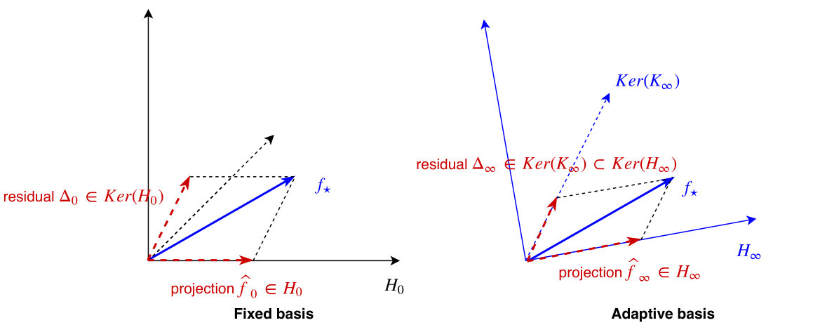 Figure 1
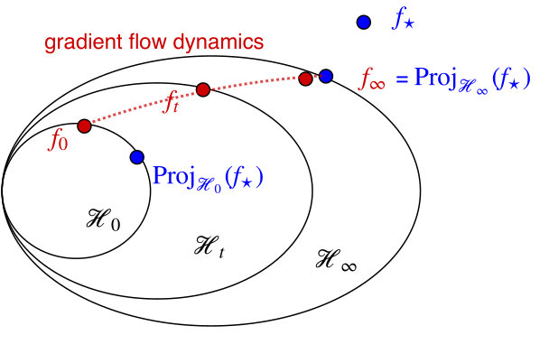 Figure 2
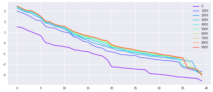 Figure 3
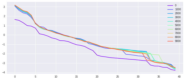 Figure 4
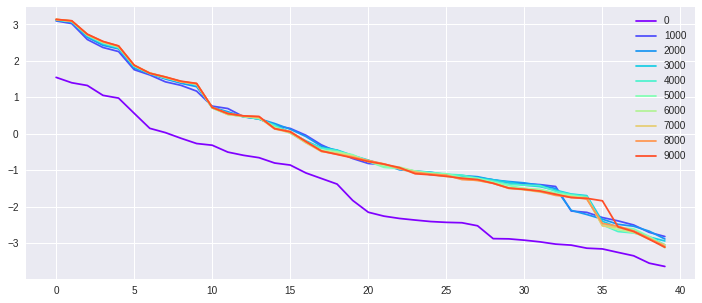 Figure 5
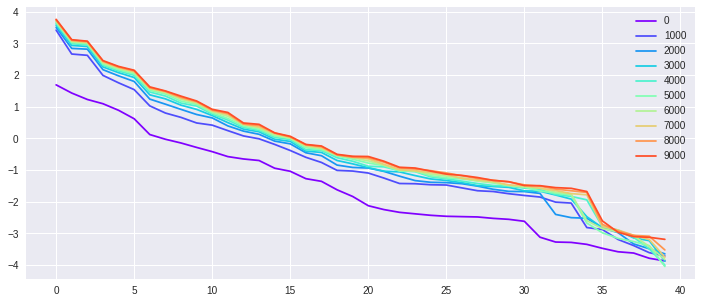 Figure 6
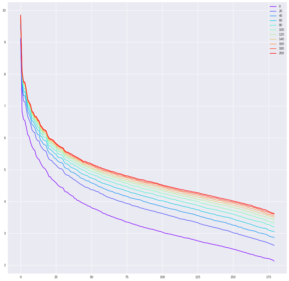 Figure 7
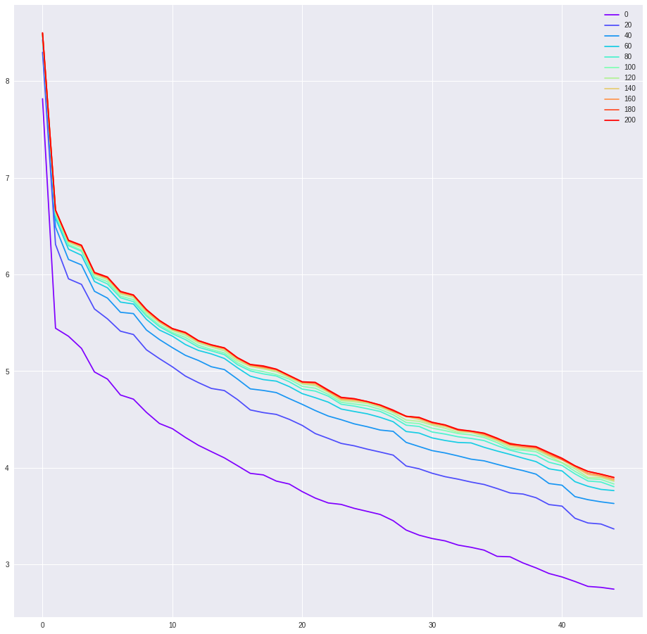 Figure 8
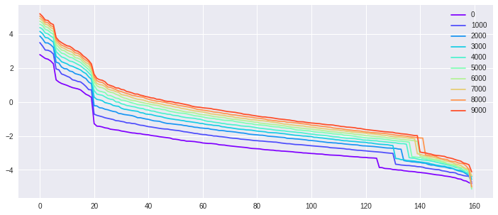 Figure 9
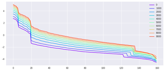 Figure 10
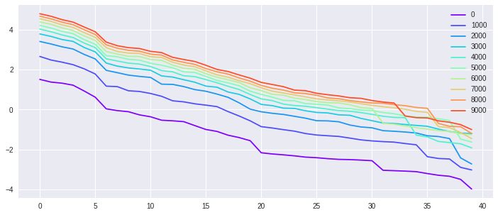 Figure 11
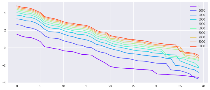 Figure 12
| finite neurons | infinite neurons | |
|---|---|---|
| finite samples | Interpolation (finite rank kernel, Thms. 3.1, 3.2 & Prop. 4.1) | Interpolation (finite rank kernel, Thms. 3.1, 3.2 & Prop. 4.1) |
| infinite samples | Approximation (finite rank kernel, Thms. 3.1 & 3.2) | Approximation (possibly universal kernel222Whether the kernel is universal in the case still depends on and the data distribution . See the simulations of Maennel et al. [2018]., Thms. 3.1 & 3.2) |
Peer Reviews
No public reviews on file for this paper yet. If you reviewed it on a platform where reviews are public (OpenReview, ICLR, NeurIPS, ICML), you can paste yours below so the community can read it here.
Videos
No videos yet. Explain this paper in a talk, walkthrough, or lecture? Add one.
Training Neural Networks as Learning Data-adaptive Kernels: Provable Representation and Approximation Benefits
Xialiang Dou
Department of Statistics, University of Chicago
Tengyuan Liang
Booth School of Business, University of Chicago
Liang gratefully acknowledges support from the George C. Tiao Fellowship.
Abstract
Consider the problem: given the data pair drawn from a population with , specify a neural network model and run gradient flow on the weights over time until reaching any stationarity. How does , the function computed by the neural network at time , relate to , in terms of approximation and representation? What are the provable benefits of the adaptive representation by neural networks compared to the pre-specified fixed basis representation in the classical nonparametric literature? We answer the above questions via a dynamic reproducing kernel Hilbert space (RKHS) approach indexed by the training process of neural networks. Firstly, we show that when reaching any local stationarity, gradient flow learns an adaptive RKHS representation and performs the global least-squares projection onto the adaptive RKHS, simultaneously. Secondly, we prove that as the RKHS is data-adaptive and task-specific, the residual for lies in a subspace that is potentially much smaller than the orthogonal complement of the RKHS. The result formalizes the representation and approximation benefits of neural networks. Lastly, we show that the neural network function computed by gradient flow converges to the kernel ridgeless regression with an adaptive kernel, in the limit of vanishing regularization. The adaptive kernel viewpoint provides new angles of studying the approximation, representation, generalization, and optimization advantages of neural networks.
Keywords: adaptive estimation, neural networks, reproducing kernel Hilbert space, gradient flow dynamics, representation learning, algorithmic approximation, interpolation.
1 Introduction
Consider i.i.d. data pairs drawn from a joint distribution on the space . At the intersection of statistical learning theory [Vapnik, 1998] and approximation theory [Cybenko, 1989], the following approximation problem requires to be first understood, before any further statistical results to be established. For a model class , one is interested in whether there exists such that the population squared loss is small,
[TABLE]
with the conditional expectation (or Bayes estimator) defined as . Eqn. (1.1) generally reads as approximating in the mean squared error sense.
Statistically, researchers approach the above question mainly in two ways. The first is by assuming that the conditional expectation lies in the correct model class . For example, say consists of linear models or splines with a particular order of smoothness, or more broadly functions lying in a reproducing kernel Hilbert space (RKHS). Conceptually, this “well-specification” assumption requires substantial knowledge about what model class might be suitable for the regression task at hand, which is often unavailable in practice. Within each framework, minimax optimal rates and extensive study have been established in [Stone, 1980, Wahba, 1990]. The second way, which extends the first approach further, considers all under some mild conditions. Building upon certain universal approximation theorem, one studies a sequence of model classes called sieves with changing [Geman and Hwang, 1982], such that the class contains an -approximation to any under some metric. A final result usually requires a careful balancing of the approximation and stochastic error by tuning . Particular cases for the latter approach include polynomials (Stone-Weierstrass, Bernstein), radial-basis [Park and Sandberg, 1991, Niyogi and Girosi, 1996], and two-layer and multi-layer neural networks [Cybenko, 1989, Hornik et al., 1989, Anthony and Bartlett, 2009, Rahimi and Recht, 2008, Daniely et al., 2016, Bach, 2017, Farrell et al., 2018, Koehler and Risteski, 2018, Poggio et al., 2017].
However, the following significant drawbacks of the above current theory make it inadequate to present an adaptive and realistic explanation of the practical success of neural networks. Firstly, the function computed in practice could be very different from that claimed in the approximation theory, either by the existence or by constructions. To see this, consider the multi-layer neural networks. It is hard to conceive that the function, computed in practice via now-standard stochastic gradient descent (SGD) training procedure, is close to the one asserted by the universal approximation results. Secondly, in practice, researchers usually explore different model classes to learn which representation best suits the data. For example, using different kernels machines, random forests, or specify certain architectures then run SGD on neural networks. In this case, strictly speaking, the choice of the model class depends on the data in an adaptive way, without prior knowledge about the basis. There have been substantial advances made to address the above two concerns — for instance, Jones [1992] on the first and Huang et al. [2008], Barron et al. [2008] on the second — for being a linear span of a library of candidate functions (union of various set of basis that can be correlated), with greedy selection rules. Nevertheless, the current theory still falls short of describing the approximation and adaptivity for the non-convex and possibly non-smooth gradient descent training on all-layer weights of the neural networks, as done in practice.
We take a step to bridge the above mismatch in the current theory and practice for neural networks and to establish a theoretical framework where the model classes adapt to the data. In particular, we answer the following algorithmic approximation question:
Given data pair , denote . Specify a neural networks model, and run gradient flow until any stationarity (). Denote the computed function to be . How does relate to , in terms of approximation and representation?
Also, we aim to formalize and shed light on the representation benefits of neural networks:
What are the provable benefits of the adaptive representation learned by training neural networks compared to the classical nonparametric pre-specified fixed basis representation?
The intimate connection between two-layer neural networks and reproducing kernel Hilbert spaces (RKHS) has been studied in the literature, see Rahimi and Recht [2008], Cho and Saul [2009], Daniely et al. [2016], Bach [2017], Jacot et al. [2018]. However, to the best of our knowledge, known results are mostly based on a fixed RKHS (in our notation in Section 5.1). In that sense, random features for kernel learning [Rahimi and Recht, 2008, 2009, Rudi and Rosasco, 2017] can be viewed as neural networks with fixed random sampled first layer weights, and tunable second layer weights. From the neural networks side, Rotskoff and Vanden-Eijnden [2018], Mei et al. [2018], Sirignano and Spiliopoulos [2019] study the mean-field theory for two-layer neural networks, and Jacot et al. [2018], Du et al. [2018], Chizat and Bach [2018], Ghorbani et al. [2019] study the linearization of neural networks around the initialization and draw connections to RKHS in various over-parametrized settings. In contrast, we will establish a general theory with the dynamic and data-adaptive RKHS obtained via training neural networks, with standard gradient flow on weights of both layers. Connections and distinctions to the literature that motivates our study are further discussed with details in Section 5. As a distinctive feature of the adaptive theory, we emphasize that all is considered, without pre-specified structural assumptions.
1.1 Problem Formulation
In this paper, we consider the time-varying function to approximate , parametrized by a two-layer rectified linear unit (ReLU) neural network (NN).
[TABLE]
The time index corresponds to the evolution of parameters driven by the gradient flow/descent (GD) training dynamics. Here each individual pair in the summation is associated with a neuron. Consider the gradient flow as the training dynamics for the weights of the neurons: for the loss function and the random variable , the parameters evolve with time as follows
[TABLE]
Equivalently, we can rewrite the function computed by NN at time as
[TABLE]
where is a signed combination of delta measures. We will define a careful rescaling of denoted as (Eqn. (5.8)), then derive the corresponding distribution dynamic for driven by the gradient flow later in Section 5.2. The rescaled formulation naturally extends to the infinite neurons case with .
In this paper, by considering various distributions of , we study two following problems: approximation and empirical risk minimization (ERM).
Function Approximation: The data pair is sampled from the population joint distribution. We are going to answer how approximates in function spaces, induced by the gradient flow on neuron weights
[TABLE]
Here we denote , and remark that all are considered without additional assumptions.
ERM and Interpolation: The data pair follows the empirical distribution. We will study gradient flow for the ERM
[TABLE]
In this case, the target reduces to with as the empirical expectation. When the minimizer of Eqn. (1.6) achieves the zero loss, we call it the interpolation problem [Zhang et al., 2016, Belkin et al., 2018b, Ma et al., 2017, Liang and Rakhlin, 2018, Rakhlin and Zhai, 2018, Belkin et al., 2018a]. Here we are interested in when and how interpolates , for .
Finally, we remark that in practice, extending the gradient flow results to the (1) positive step size GD, and (2) mini-batch stochastic GD, are standalone interesting research topics. The reasons are that the optimization is non-smooth for the ReLU activation and that the interplay between the batch size and step size is less transparent in non-convex problems.
2 Preliminaries and Summary
2.1 Notations
We use the boldface lower case to denote a random variable or vector. The normal letter can either be a scaler or a vector when there is no confusion. The transpose of a matrix , resp. vector is denoted by , resp. . denotes the Moore–Penrose inverse. For , let . We use to denote the -th entry of a matrix. We denote as the indicator function of set . We call symmetric positive semidefinite functions kernels, and use calligraphy letter to denote Hilbert spaces. We use to denote the inner product in (or ). denotes the empirical distribution for . Notation is the expectation w.r.t random variable , and . For a signed measure with the positive and negative parts, define .
2.2 Preliminaries
We use the signed measure , defined by the neuron weights at training time collectively, to construct a dynamic RKHS. The mathematical definition of is deferred to Section 5.1 and 5.2 (specifically, Eqn. (5.8)). The stationary signed measure at is denoted as . For completeness we walk through the construction of the dynamic kernel and RKHS with . Define the linear operator , such that for any
[TABLE]
One can define the adjoint operator , such that for ,
[TABLE]
Note that both and are compact operators under the finite total variation and compact support assumptions. For the finite neurons case (1.2), the operator is of finite rank. We define the compact integral operator with the corresponding kernel
[TABLE]
The dynamic RKHS can be readily constructed via . Let the eigen decomposition of be the countable sum Here can be a nonnegative integer or , and . without confusion can represent either an eigen function or a linear functional. Similarly, we have the singular value decomposition for and as well. For a detailed discussion, see e.g. Casselman [2014]. Again, is a function in or a linear functional. The RKHS can be specified as follows.
[TABLE]
We refer to as the stationary RKHS kernel, and as the stationary RKHS. One can view that the gradient flow training dynamics — on the parameters of NN — induces a sequence of functions and dynamic RKHS , indexed by the time .
2.3 Organization and Summary
We will prove three results, which are summarized informally in this section (see also Table 1). We remark that Theorems 3.1 and 3.2 are stated for the approximation problem. However, as done in Corollary 3.1, by substituting by the empirical counterparts, one can easily state the analog for the ERM problem. Recall .
Gradient flow on NN converges to projection onto data-adaptive RKHS. Theorem 3.1 shows that as done in practice training NN with simple gradient flow, in the limit of any local stationarity, learns the adaptive representation, and performs the global least squares projection simultaneously. Define as the function computed by ReLU networks (defined in (1.2), or more generally in (5.9)) until any stationarity of the gradient flow dynamics (defined in (1.3), with the squared loss) for the population distribution . Define the corresponding stationary RKHS (defined in (2.1)).
[Informal version of Thm. 3.1] Consider , for any local stationarity of the gradient flow dynamics (1.3) on the weights of neural networks (1.2), the function computed by NN at stationarity satisfies
[TABLE]
Representation benefits of data-adaptive RKHS. Theorem 3.2 illustrates the provable benefits of the learned data-adaptive representation/basis . We emphasize that , as obtained by training neural networks on the data , depends on the data in an implicit way such that there are advantages of representing and approximating .
[Informal version of Thm. 3.2] Consider and the same setup as Theorem 3.1. Decompose into the function computed by the neural network and the residual
[TABLE]
Then there is another RKHS (defined in (3.4)) , such that
[TABLE]
with a gap in the spaces .
Convergence to Ridgeless regression with adaptive kernels. Proposition 4.1 establishes that in the vanishing regularization limit, the neural network function computed by gradient flow converges to the kernel ridgeless regression with an adaptive kernel (denoted as ). Consider using the gradient flow on the weights of the neural network function , to solve the -regularized ERM
[TABLE]
Denote the function computed by NN at any local stationarity of ERM as , we answer the extrapolation question at a new point , with the generalization error discussed in Prop. 4.2. The result is extendable to the infinite neurons case.
[Informal version of Prop. 4.1] Consider only the bounded assumption on initialization that for all . At stationarity, denote the corresponding adaptive kernel as . The neural network function has the following expression,
[TABLE]
3 Main Results: Benefits of Adaptive Representation
We formally state two main results of the paper, Theorem 3.1 and Theorem 3.2 below.
3.1 Gradient Flow, Projection and Adaptive RKHS
We study how the function computed from gradient flow on NN represents when reaching any stationarity, under the squared loss. Consider the gradient flow dynamics (5.3) reaching any stationarity. Assume that the corresponding signed measure in (5.8) satisfies with a compact support. The mathematical details about are postponed to Section 5.2. We employ the notation since reaching stationarity can be viewed as .
We would like to emphasize that this stationary signed measure is task adaptive: it implicitly depends on the regression task and the data distribution , rather than being pre-specified by the researcher as in Bach [2017], Daniely et al. [2016], Cho and Saul [2009]. With the RKHS established in Section 2.2, we are ready to state the following theorem.
Theorem 3.1** (Approximation).**
For any conditional mean , consider solving the approximation problem (1.5), with the ReLU NN function defined in (1.2) where and are the weights for . For any signed measure with , consider the infinitesimal initialization weights , and , with sampled independently. When the training dynamics (1.3) reaches any stationarity, it defines a stationary signed measure (on the collective weights) with , and a corresponding stationary RKHS with the kernel defined in Eqn. (2.1), such that:
the function computed by neural networks at stationarity has the form
[TABLE] 2. 2.
* is a global minimizer of approximating within the RKHS *
[TABLE]
In addition, the same results extend to the infinite neurons case with where the limit for can be defined in the weak sense.
Remark 3.1**.**
The above theorem shows that obtained by training on two-layer weights over time until any stationarity, is the same as projecting onto the stationary RKHS . The projection is the solution to the classic nonparametric least squares, had one known the adaptive representation beforehand. Conceptually, this is distinct from the theoretical framework in the current statistics and learning theory literature: we do not require the structural knowledge about (say, smoothness, sparsity, reflected in ). Instead, we run gradient descent on neural networks to learn an adaptive representation for , and show how the computed function represents in this adaptive RKHS .
In other words, as done in practice training NN with simple gradient flow, in the limit of any local stationarity, learns the adaptive representation, and performs the global least-squares projection simultaneously. Training NN is learning a dynamic representation (quantified by ), at the same time updating the predicted function , as shown in Fig. 1.
A final note on the infinite neuron case: for any fixed time , with the proper random initialization, setting defines a proper distribution dynamics on the weak limit shown in Lemma 5.3. Then set to obtain the stationarity RKHS .
From the above, we have the following natural decomposition,
[TABLE]
Surprisingly, as we show in the next section, actually lies in a smaller subspace of , characterized by . We call this the representation and approximation benefits of the data-adaptive RKHS learned by training neural networks.
Before moving next, we briefly discuss the above theorem when applied to the empirical measure, to solve the ERM problem. First, as a direct corollary, the following holds.
Corollary 3.1** (ERM).**
Consider the ERM problem (1.6), with the other settings the same as in Theorem 3.1. One can define the finite dimensional RKHS (at most rank ) as in (2.1) with substituting . When reaches any stationarity, the solution satisfies
[TABLE]
More importantly, we will show in Proposition 4.1 that the function computed by training neural networks with gradient descent on the empirical risk objective until any stationarity (with vanishing regularization), can be shown to be the kernel ridgeless regression with the data-adaptive RKHS . Hence, studying the out of sample performance for GD on NN reduces to the generalization of kernel ridgeless regression with adaptive kernels.
3.2 Representation Benefits of Adaptive RKHS
We now define another adaptive RKHS named as the GD kernel, which turns out to be different from in (2.1). Interestingly, the difference in these two kernels sheds light on the representation benefits of the adaptive RKHS. The new RKHS is motivated by the gradient training dynamics. Recall the associated signed measure at the stationarity, The GD kernel is defined as
[TABLE]
which is different than the stationary RKHS kernel in (2.1). We use to denote the integral operator associated with ,
[TABLE]
With a slight abuse of notation, we denote the corresponding RKHS to be as well. Now we are ready to state the main theorem on the representation benefits.
Theorem 3.2** (Representation Benefits).**
Consider and the same setting as in Theorem 3.1. Consider the approximation problem (1.5) with either finite or infinite neurons, and the gradient flow dynamics (5.3) (equivalently (1.3)) with data pair drawn from the population distribution. When reaching any stationary signed measure , is decomposed into the function computed by the neural network and the residual
[TABLE]
Recall the RKHS in (2.1) and the GD RKHS in (3.4), all learned from the data and adaptively. The following holds,
[TABLE]
with . In other words, GD on NN decomposes into two parts, and each lies in a space that is NOT the orthogonal complement to the other.
Remark 3.2**.**
As we can see and are not the same. Therefore, the decomposition is not a trivial orthogonal decomposition to the RKHS and its complement.
Recall Theorem 3.1, projecting to the RKHS with the data-adaptive kernel
[TABLE]
associated with is the same as the function constructed by neural networks (GD limit as ). However, the residual lies in a possibly much smaller space due to Theorem 3.2, which is the null space of the RKHS
[TABLE]
In other words, as the learned adaptive basis (from GD) depends on the data distribution and the task implicitly, it has the advantage of representing by squeezing the residual into a smaller subspace in the null space of . A pictural illustration can be found in Fig. 2. This representation and approximation benefit helps with explaining the better interpolation results obtained by neural networks [Zhang et al., 2016, Belkin et al., 2018b, Liang and Rakhlin, 2018, Belkin et al., 2018a]: (1) the adaptive basis is tailored for the task , thus the residual/interpolation error lies in a smaller space; (2) in view of the ODE in Corollary 5.2, the second layer of NN adds implicit regularization to the smallest eigenvalues of , thus improving the converging speed of to zero.
Before concluding this section, we remark that a similar result holds for the ERM problem (1.6). As we shall discuss in the next section, the gap between and can be large, even for the ERM problem.
4 Implications of the Adaptive Theory
In this section, we will discuss some direct implications of the adaptive kernel theory for neural networks established in this paper.
Example: Gap in Spaces and .
In Theorem 3.2, it is established that . We now construct a concrete case to illustrate the potentially significant gap in these two spaces as follows. Consider only one neuron with , solving ERM problem (1.6) with samples, and with dimension . In this case, is supported on only one point, noted as . Denote as the data matrix, one can show that
[TABLE]
has rank . In contrast,
[TABLE]
can be of rank . Hence the null space of is much smaller than that of . The gap can be large for many other settings of .
Connections to Min-norm Interpolation.
The following result establishes the connections between the solution of gradient descent on neural networks (at local stationarity), and the kernel ridgeless regression [Belkin et al., 2018b, Liang and Rakhlin, 2018, Hastie et al., 2019] with an adaptive kernel . Empirical evidence on the similarity between the interpolation with kernels and neural networks was discovered in Belkin et al. [2018b]. The following proposition provides a novel way of studying the generalization property of neural networks via adaptive kernels.
Proposition 4.1** (Interpolation: Connection to Kernel Ridgeless Regression).**
Consider the gradient flow dynamics on all the weights of the neural network function , to solve the -regularized ERM
[TABLE]
Consider only the bounded assumption on initialization that for all . At stationarity, denote the signed measure as and the corresponding adaptive kernel as . Then the neural network function at stationarity satisfies,
[TABLE]
In the vanishing regularization limit, the neural network function converges to the kernel ridgeless regression with the adaptive kernel, when exists,
[TABLE]
Note that the generalization theory for the kernel ridgeless regression has been established Liang and Rakhlin [2018], Hastie et al. [2019]. Here the kernel is data-adaptive (that adapts to ) learned along training, instead of being fixed and pre-specified.
Connections to Random Kitchen Sinks.
Let us introduce two function spaces, with the base measure (fixed representation)
[TABLE]
[TABLE]
In random kitchen sinks studied in Rahimi and Recht [2008, 2009], by assuming that lies in the RKHS, the approximation error can be controlled by the existence of the following function with i.i.d. sampled from
[TABLE]
Note that lies in a possibly much larger space though the target only lies in . Similarly for two-layer neural networks function considered in [Bach, 2017, Section 2.3], the RKHS space can be more restrictive compared to .
In contrast, with the adaptive RKHS representation , we have shown that
[TABLE]
The extreme case of fully adaptive function space is defined with tailored for , . The adaptive representation learned by neural networks can be viewed as in between the fixed and the fully adaptive representation.
Adaptive Generalization Theory.
Now we attempt to provide a new decomposition to study the generalization of NN via adaptive kernels. Recall we have shown that where Define the population limit and . Denote the ridgeless regression with the population adaptive kernel ,
[TABLE]
Assume a.s. (can be relaxed). One can derive the following decomposition for generalization.
Proposition 4.2** (Adaptive Generalization).**
[TABLE]
Note this result holds without requiring global optimization guarantees. The first term is the representation error, which corresponds to the closeness of the adaptive RKHS (using empirical distribution) and (using population distribution). The second term is the adaptive approximation error studied in the current paper. The third and fourth terms are the variance and bias expressions studied in Liang and Rakhlin [2018], Hastie et al. [2019], Rakhlin and Zhai [2018], as if assuming the actual function lies in . This decomposition suggests the possibility of studying generalization without explicit global understanding of the optimization, and providing rates that adapts to without structural assumptions.
5 Time-varying Kernels and Evolution
In this section, we lay out the mathematical details on the time-varying kernels and the evolution of the signed measure supporting the main results. In the meantime, we will discuss in depth the relevant literature motivating our proof ideas.
First, we describe the motivation behind the dynamic RKHS , and the GD kernel induced by the gradient descent dynamics. Extensions to multi-layer perceptrons is in Sec. A.2.
Lemma 5.1** (Dynamic kernel of finite neurons GD).**
Consider the approximation problem (1.1) with a neural network function (1.2), and the training process (1.3) with population distribution. Let be the residual. Define the time-varying kernel ,
[TABLE]
Then the residual driven by the GD dynamics satisfies,
[TABLE]
When running GD to solve the empirical risk minimization (ERM), the dynamics of the finite-dimensional sample residual has been established in Jacot et al. [2018], Du et al. [2018]. Here we generalize the result to optimize the weights of both layers, and to solve the infinite-dimensional population approximation problem rather than the empirical risk minimization problem. For a general loss function with curvature (say, logistic loss), similar results hold under slightly stronger conditions.
Corollary 5.1**.**
Consider a general loss function that is -strongly convex in the second argument , with defined in (5.1). Assume in addition has smallest eigenvalue . Define , then we have for all ,
[TABLE]
5.1 Initialization, Rescaling and
Now we describe the initialization and rescaling schemes used in the main theorems. Rewrite (1.1) according to the signs of the second layer weights
[TABLE]
Initialization.
We consider the “infinitesimal” initialization drawn from two probability measures and that do not depend on :
[TABLE]
Here with . The rescaling factor turns out to be crucial when defining the infinite neurons limit for the evolution of signed measures. Remark that such initialization is w.l.o.g., and accounts for the infinitesimal nature used in practice when the number of neurons grows. For the second layer weights, we impose the “balanced condition” motivated by Maennel et al. [2018],
[TABLE]
It turns out that with such initialization, the balanced condition holds throughout the training process induced by gradient flow, which is useful for the main theorems. Interestingly, in the proof of Proposition 4.1, we show that such balanced condition always holds at stationarity when training neural networks with regularization, even for unbalanced initialization.
Proposition 5.1** (Balanced condition).**
For , , and , and the initialization specified above, at any time , we have
[TABLE]
Rescaling.
To prepare for the distribution dynamic theory in the next section, we introduce a parameter rescaling with the factor. Let and , also define and sampled from and at . Under this representation,
[TABLE]
By the positive homogeneity of ReLU, we have the corresponding dynamics on the rescaled parameters,
[TABLE]
Define at time
[TABLE]
as the empirical distribution over neurons on the parameter space . The and converge weakly to proper distributions in the infinite neurons limit , see e.g. Bach [2017], Mei et al. [2018]. Through the balanced condition in Proposition 5.1 and Proposition A.1, we know (by substituting by )
[TABLE]
The above motivates the study of the RKHS as in Theorem 3.1, with the kernel
[TABLE]
To conclude this section, we provide the explicit formula for the initial kernel matrix under such infinitesimal random initialization. Specifically, consider the initialization with being with equal chance and sampled. The initial kernel has the following expression, in the infinite neurons limit.
Lemma 5.2** (Fixed Kernel).**
With initialization specified above, consider w.l.o.g. , and denote as the isotropic Gaussian . By the strong law of large number, we have almost surely,
[TABLE]
Much known results [Bengio et al., 2006, Rahimi and Recht, 2008, Bach, 2017, Cho and Saul, 2009, Daniely et al., 2016] on the connection between RKHS and two-layer NN focus on some fixed kernel, such as . To instantiate useful statistical rates, one requires to lie in the corresponding pre-specified RKHS , which is non-verifiable in practice. In contrast, the dynamic kernel is less studied. We will establish a dynamic and adaptive kernel theory defined by GD, without making any structural assumptions on other than .
5.2 Evolution of
In this section, we derive the evolution of the signed measure defined by the neurons at the training , which in turn determines the dynamic kernel defined in (5.1). To generalize the result to the case of infinite neurons, we follow and borrow tools from the mean-field characterization [Mei et al., 2018, Rotskoff and Vanden-Eijnden, 2018, Jordan et al., 1998]. The rescaling described in the previous section proves handy when defining such infinite neurons limit. We define the velocity field driven by the regression task and the interaction among neurons,
[TABLE]
The following theorem casts the training process as distribution dynamics on .
Lemma 5.3** (Dynamic Kernel and Evolution).**
Consider the approximation problem (1.1), and the gradient flow as the training dynamic (1.3). For , and defined in (5.8) with possibly infinite neurons, we have the following PDE characterization on distribution dynamics of
[TABLE]
Moreover, the GD kernel is defined as
[TABLE]
Remark 5.1**.**
As in Mei et al. [2018], Rotskoff and Vanden-Eijnden [2018], let’s first show that in the infinite neurons limit , are properly defined, with Eqn. (5.3) characterizing the distribution dynamics. For simplicity, we assume the initialization is with bounded support. Add the superscript , to (5.8) to indicate their dependence on . Consider that , in (5.11) are bounded and uniform Lipchitz continuous as in [Mei et al., 2018, A3]. With the same proof as in [Mei et al., 2018, Theorem 3], one can show that with , the initial distribution by law of large number. And by the solution’s continuity w.r.t. the initial value, we have as well defined, for any fixed .
Note that our problem setting is slightly different from that in Mei et al. [2018], where the authors consider the NN with fixed second layer weights to be . We reiterate that the re-parameterization via and is crucial: (1) weights on both layers are optimized following the gradient flow; (2) infinitesimal random initialization is employed in practice. In the setting of [Mei et al., 2018, Eqn. (3)], the training process is slightly different from the vanilla GD on weights, with an additional factor in the velocity term. This subtlety is also mentioned in Rotskoff and Vanden-Eijnden [2018]. In short, the rescaling looks at the dynamics where ’s are on the invariant scale as for any fixed effective time (that does not depend on ). Here we analyze the exact gradient flow on the two-layer weights, with infinitesimal random initialization as in practice, resulting in a different velocity field (5.11) compared to that in Mei et al. [2018].
The proof of Theorem 3.1 makes use of (5.9)-(5.10) and the stationary condition implied by Lemma 5.3. The balanced condition is crucial in both Theorem 3.1 and Proposition 4.1. The details of the proof are deferred to Section 7.
5.3 Two RKHS: and
In this section we compare the two adaptive RKHS appeared in (5.13), and in (5.10). The comparison will lead to the proof of Theorem 3.2. We start with generalizing Lemma 5.1 with the possibly infinite neurons case via the distribution dynamics in (5.3).
Corollary 5.2**.**
Consider the same setting as in Lemma 5.1 with possibly infinite neurons NN (5.9), and the training process (5.3). Define the time-varying kernel matrix , with the signed measure follows (5.3)
[TABLE]
Then we still have
It turns out that the kernels and , defined in (3.4) and (2.1) respectively, satisfy the following inclusion property.
Proposition 5.2**.**
Consider the training process reaches any stationarity with compact support within radius and finite total variation. We have
[TABLE]
with defined in (5.14). Combining with the fact that implies
[TABLE]
The proof of Theorem 3.2 uses the following fact: when reaching stationarity, due to the ODE defined by GD in Lemma 5.1, the residual must satisfy
[TABLE]
The proof of Proposition 5.2 and Theorem 3.2 are deferred to Section 7.
6 Experiments
We run experiments to illustrate the spectral decay of the dynamic kernels defined in over time . The exercise is to quantitatively showcase that during neural network training, one does learn the data-adaptive representation, which is task-specific depending on the true complexity of . The training process is the same as the one we theoretically analyze: vanilla gradient descent on a two-layer NN of neurons, with infinitesimal random initialization scales as .
The first experiment is a synthetic exercise with well-specified models. We generate from isotropic Gaussian in , and with different . In other words, we choose different target (task complexity) by varying . We select in our experiment. The top of the sorted eigenvalues of the kernel matrix along the GD training process are shown in Fig. 3. The -axis is the index of eigenvalues in descending order, and the -axis is the logarithmic values of the corresponding eigenvalues. Different color indicates the spectral decay of the at different training time . The eigenvalue-decays stabilize over time means that the training process approaches stationarity. As we can see with belongs to the NN family, the eigenvalues of the kernel matrix, in general, become larger during the training process. For a more complicated target function, it takes longer to reach stationarity.
The second experiment is another synthetic test on fitting random labels. We generate from isotropic Gaussian in , as takes with equal chance. We select , and to investigate those parameters’ influence on the kernel . We want to point out two observations. First, fixed , we investigate over-parametrized models ( large). Shown from Fig. 4 along the row, the kernels for different ’s behave much alike. In other words, in the infinite neurons limit, the kernel will stabilize. Second, fixed , we vary the number of samples , to simulate different interpolation hardness. As seen from Fig. 4 along the column, the kernels and the convergence over time are distinct, reflecting the different difficulty of the interpolation.
The third experiment (Fig. 5) is regression using the MNIST dataset with different sample size . We hope to investigate the influence of sample size on the kernel matrix along the training process. For a larger sample size , it takes longer to reach stationarity.
7 Main Proofs
Proof of Theorem 3.1.
From the definition, we have for any , and is a surjective mapping. Suppose that is a minimizer of (3.2), then we claim that for any , one must have
[TABLE]
This claim can be seen from the following argument. Suppose not, then for that violates the above, construct
[TABLE]
we know
[TABLE]
For with the same sign as and small enough, one can see that which validates that is a minimizer. From the same argument, one can see that is a minimizer if and only if (7.1) holds, in other words,
[TABLE]
From PDE characterization (5.3) with ReLU activation, one knows that
[TABLE]
and the expression for the velocity field
[TABLE]
We know that any stationary point has the following property [Mei et al., 2018]:
[TABLE]
Multiplying both sides by and recall the property of ReLU, the above condition implies that for all , we have
[TABLE]
One can see the stationary condition on (fixed points of the dynamics) (7.5) translates to
[TABLE]
Here the function is the Radon-Nikodym derivative. In addition, one can easily verify that, as has bounded total variation
[TABLE]
Therefore, combining all the above, one knows that
[TABLE]
and that for any
[TABLE]
We have proved that satisfies normal condition for being a minimizer to (3.2). ∎
Proof of Proposition 5.2.
The first inequality in (5.16) is trivial. For the second inequality, it suffices to show for any , , , we have
[TABLE]
The RHS equals
[TABLE]
For the last inequality, with compactness condition on , we have
[TABLE]
Therefore, .
∎
Proof of Theorem 3.2.
Let us rewrite Corollary 5.2 into
[TABLE]
here denotes the integral operator associated with ,
[TABLE]
From (7.14)
[TABLE]
we know that the RHS equals zero implies
[TABLE]
This further implies lies in the kernel of RKHS as . ∎
Proof of Proposition 4.1.
The gradients on the original parameters are,
[TABLE]
Clearly, on the rescaled parameter, the following holds
[TABLE]
Multiply the first equation by , and the second equation by , take the difference, we can verify that
[TABLE]
Therefore the balanced condition still holds at stationarity for arbitrary bounded initialization,
[TABLE]
Now the optimality condition for the velocity field reads the following, for any (we abbreviate the in the following display, note corresponds to the second layer weights w.r.t. to )
[TABLE]
where the last step uses the condition , and the fact that and
[TABLE]
In the matrix form, where
[TABLE]
Therefore, define , and , we have
[TABLE]
The last line follows as .
∎
Proof of Proposition 4.2.
[TABLE]
For the first term, we can upper bound by . The second term can be upper bounded by
[TABLE]
Proof is completed. ∎
Acknowledgement
We thank Maxim Raginsky for pointing out relevant references, and for providing helpful discussion.
Appendix A Appendix
A.1 Supporting Results
Proof of Lemma 5.3.
Let’s first show that in the infinite neuron limit , are properly defined. Therefore Eqn. (5.3) in the above theorem also characterize the distribution dynamics for infinite neurons NN, induced by gradient flow training. For simplicity, we assume the initialization with bounded support. We add the superscript , to (5.8) to indicate their dependence on . Consider , in (5.11) are bounded and uniform Lipchitz continuous as in [Mei et al., 2018, A3]. With the same proof as in [Mei et al., 2018, Theorem 3], one can show that with , the initial distribution by law of large number, and by the solution’s continuity depending on the initial value. Therefore we have as well defined.
The velocity of a particle in the positive part as a rewrite of (5.6)-(5.7) is
[TABLE]
resp. for the negative part and (5.7), we have
[TABLE]
Given the velocity of particle, we have the transport equation for gradient flow,
[TABLE]
To see this, recall the definition of weak derivative : for any bounded smooth function , is defined in the following sense
[TABLE]
We take any bounded smooth function , given the velocity of ’s , then we have
[TABLE]
and correspondingly. By the weak derivative, we get the above PDE. We use the above dynamic description as the training process for infinite neuron NN. Plug above equation into and , we get
[TABLE]
∎
Proof of Proposition 5.1.
It suffices to show and resp. . By our path dynamics, we have
[TABLE]
Thus, by the initialization, we have , and resp. . ∎
Proposition A.1** (No sign change).**
For the training process (1.3) for problem (1.1) with NN (1.2), once and hit zero at , for at least there exists a solution that can be viewed as training without the -th neuron.
Proof of Proposition A.1.
Using , , for , as an initial value for ODE (1.3) without the -th node. By assumption, we have a solution of this -dimensional initial value problem. Then padding the solution with and , which can be a solution for ODE (1.3) with -th neuron included. ∎
Proof of Lemma 5.1.
First we write down the dynamic of prediction at each point based on Eqn. (1.3). For notational simplicity, let be , and let , and with the square loss , we have
[TABLE]
Therefore, we have
[TABLE]
∎
Proof of Corollary 5.1.
The first equality follows from the proof in Lemma 5.1. Recall the property for strongly convex function
[TABLE]
Therefore ∎
Proof of Lemma 5.2.
We know
[TABLE]
Consider the coordinate system such that spans the space of , with
[TABLE]
where . Note is still an isotropic Gaussian under this coordinate system. The constraint reads
[TABLE]
and one can see that integrate out.
Let’s focus on the spherical coordinates of , then and . W.l.o.g., we can consider the case when .
[TABLE]
Therefore, we get
[TABLE]
Similarly, we have
[TABLE]
Summing them up, we get the result. ∎
Proof of Corollary 5.2.
Our proof essentially follows the same steps for (5.1). First, we write down the dynamic of ,
[TABLE]
Plug-in the training dynamic (A.4), we get
[TABLE]
Therefore, we have
[TABLE]
∎
A.2 Extensions
In this section, we extend the definition of the dynamic kernel in Section 5 to the multi-layer neural networks case. We construct a recursive expression for the kernel defined by the multi-layer perceptron (MLP). Let , denote the coefficient from the -th node on the -th layer to the -th node on the -th layer. Let the input (before activation) of the -th node on -th layer be and let the output at that node be , for , and , for . The final output . Let and is the number of nodes at the -th layer. Denote the kernel of layers NN. The training dynamic is still the gradient flow, for all
[TABLE]
Proposition A.2**.**
For a -layer NN function denoted by , for simplicity, let
[TABLE]
With gradient flow training process, we have the following recursive representation of the corresponding kernel matrix
[TABLE]
Here the kernel matrix is always positive semidefinite.
Proof of Proposition A.2.
For notational simplicity, let , and
[TABLE]
For the proof, we calculate the dynamic of prediction , by elementary calculus, we have
[TABLE]
With same calculation for the dynamic of as in (A.7), we get
[TABLE]
By induction, we get
[TABLE]
Now, we prove the positive semi-definiteness of the kernel. By induction, we only need to prove that the second term above is non-negative. We construct a canonical mapping , whereas the -th coordinate . Then the second term can be seen as a inner product , which implies the non-negativity. ∎
The reference list from the paper itself. Each links out to its DOI / PubMed record.
- 1Anthony and Bartlett [2009] Martin Anthony and Peter L Bartlett. Neural network learning: Theoretical foundations . cambridge university press, 2009.
- 2Bach [2017] Francis Bach. Breaking the curse of dimensionality with convex neural networks. Journal of Machine Learning Research , 18(19):1–53, 2017.
- 3Barron et al. [2008] Andrew R Barron, Albert Cohen, Wolfgang Dahmen, Ronald A De Vore, et al. Approximation and learning by greedy algorithms. The annals of statistics , 36(1):64–94, 2008.
- 4Belkin et al. [2018 a] Mikhail Belkin, Daniel Hsu, Siyuan Ma, and Soumik Mandal. Reconciling modern machine learning and the bias-variance trade-off. ar Xiv preprint ar Xiv:1812.11118 , 2018 a.
- 5Belkin et al. [2018 b] Mikhail Belkin, Siyuan Ma, and Soumik Mandal. To understand deep learning we need to understand kernel learning. ar Xiv preprint ar Xiv:1802.01396 , 2018 b.
- 6Bengio et al. [2006] Yoshua Bengio, Nicolas L Roux, Pascal Vincent, Olivier Delalleau, and Patrice Marcotte. Convex neural networks. In Advances in neural information processing systems , pages 123–130, 2006.
- 7Casselman [2014] Bill Casselman. Essays in analysis. 2014.
- 8Chizat and Bach [2018] Lenaic Chizat and Francis Bach. A note on lazy training in supervised differentiable programming. ar Xiv preprint ar Xiv:1812.07956 , 2018.