A generalization of pde's from a Krylov point of view
F. Reese Harvey, H. Blaine Lawson Jr

TL;DR
This paper introduces a unified framework for generalized PDEs using subequations and Dirichlet duality, establishing existence and uniqueness conditions for solutions on bounded domains with various examples.
Contribution
It develops a comprehensive theory of generalized equations of the form f(D^2 u)=0, including existence, uniqueness, and characterization, extending classical PDE concepts via subequations and duality.
Findings
Uniqueness holds iff the generalized equation has no interior.
Existence holds iff the dual equation has no interior, with boundary convexity assumptions.
Examples include constrained Laplacian, twisted Monge-Ampère, and C^{1,1}-equation.
Abstract
We introduce and investigate the notion of a `generalized equation' of the form , based on the notions of subequations and Dirichlet duality. Precisely, a subset is a generalized equation if it is an intersection where and are subequations and is the subequation dual to . We utilize a viscosity definition of `solution' to . The mirror of is defined by . One of the main results here concerns the Dirichlet problem on arbitrary bounded domains for solutions to with prescribed boundary function . We prove that: (A)…
Click any figure to enlarge with its caption.
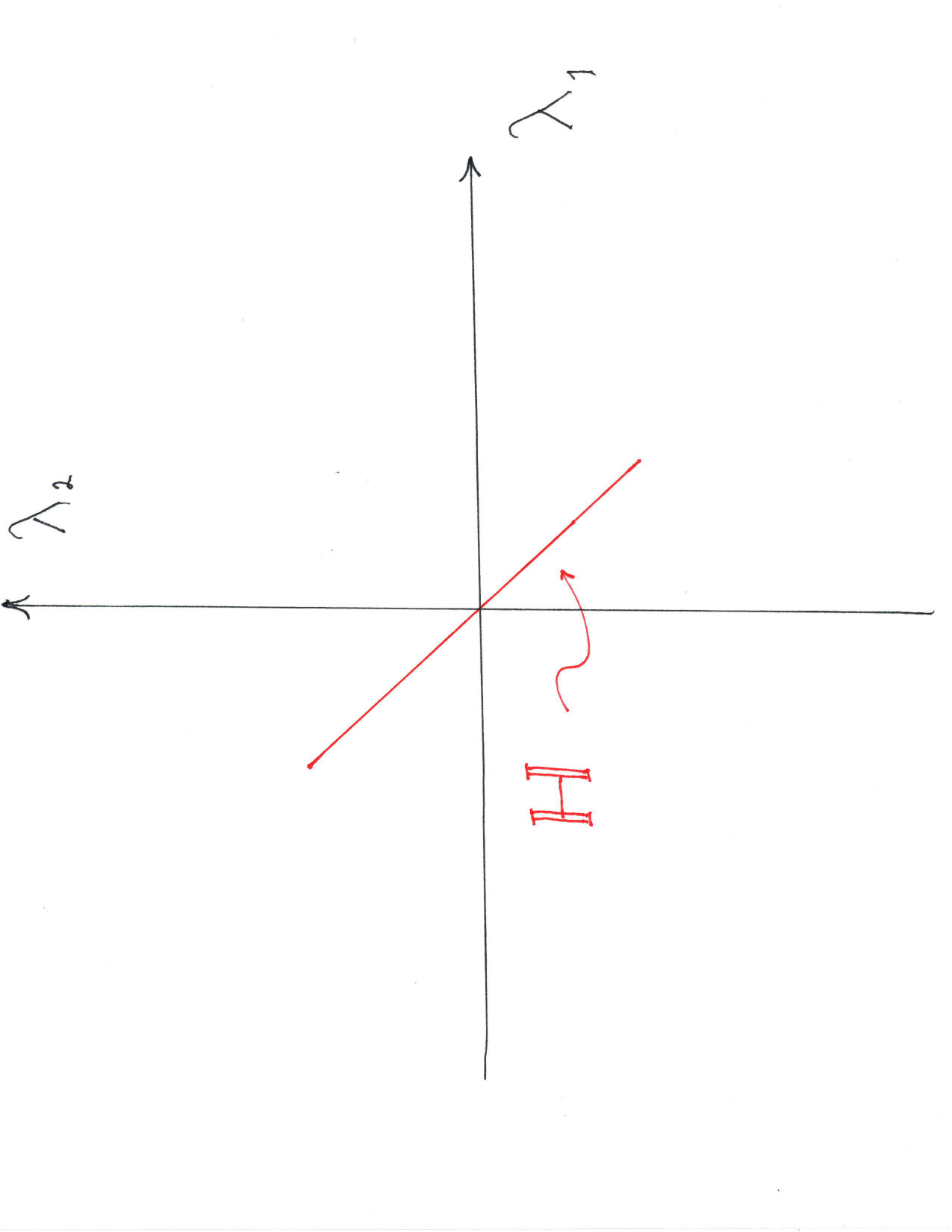 Figure 1
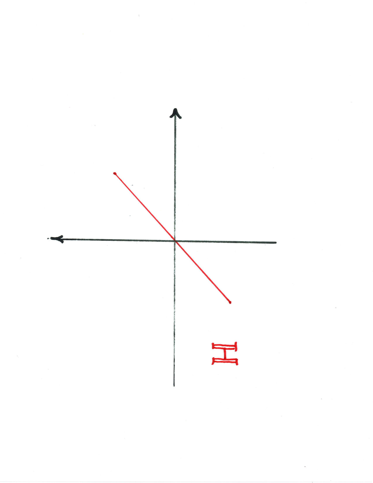 Figure 10
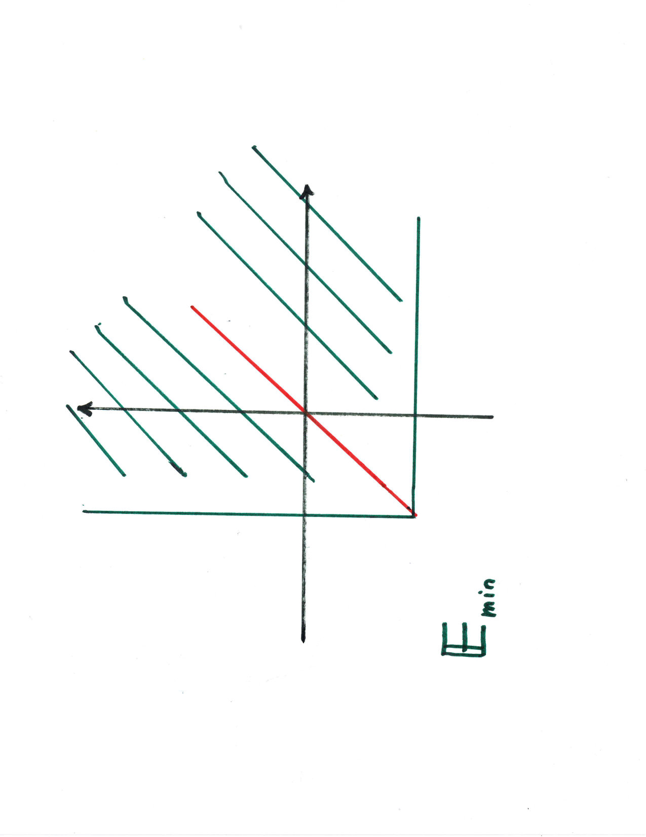 Figure 11
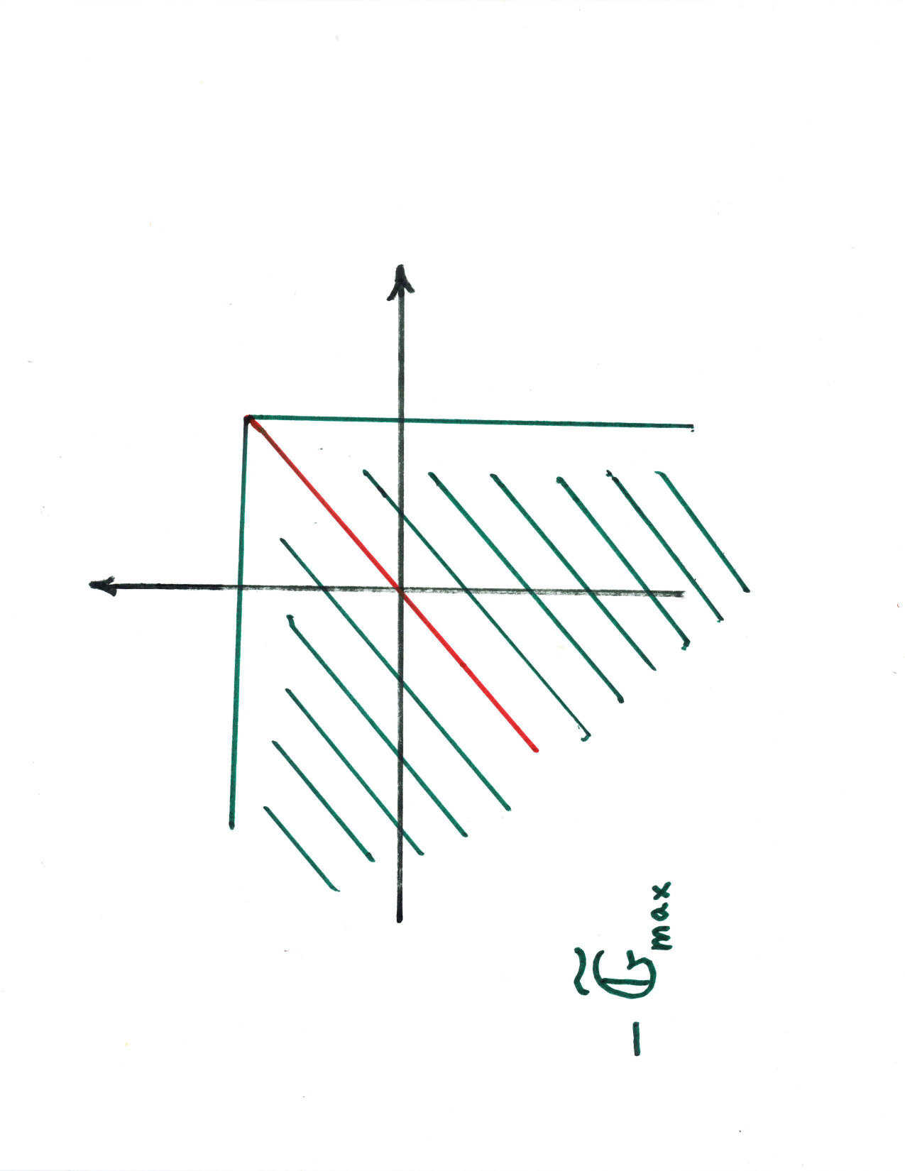 Figure 12
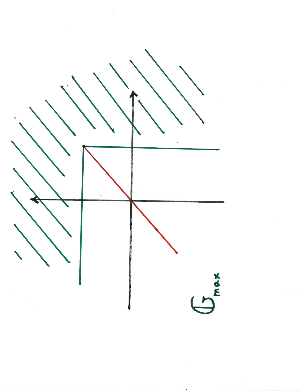 Figure 13
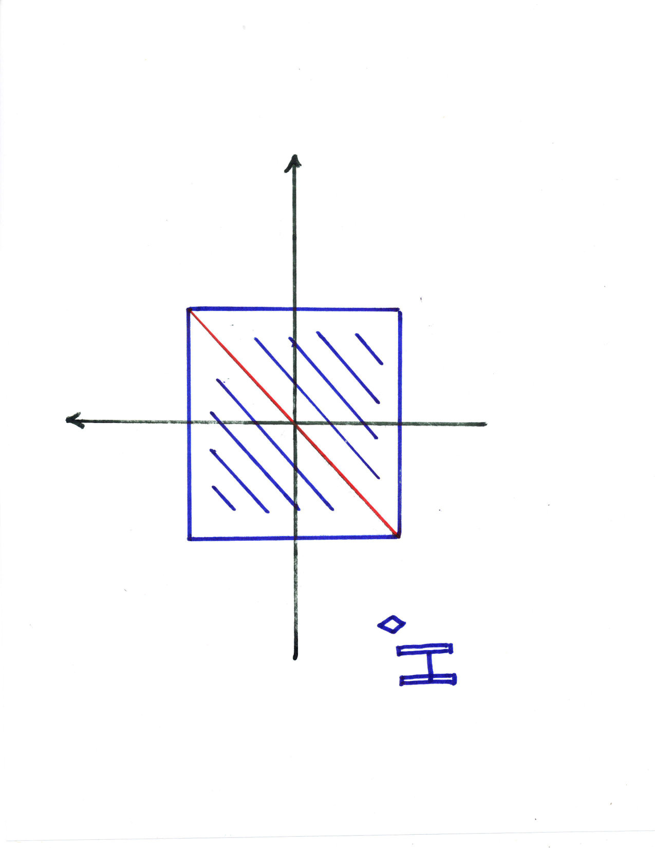 Figure 14
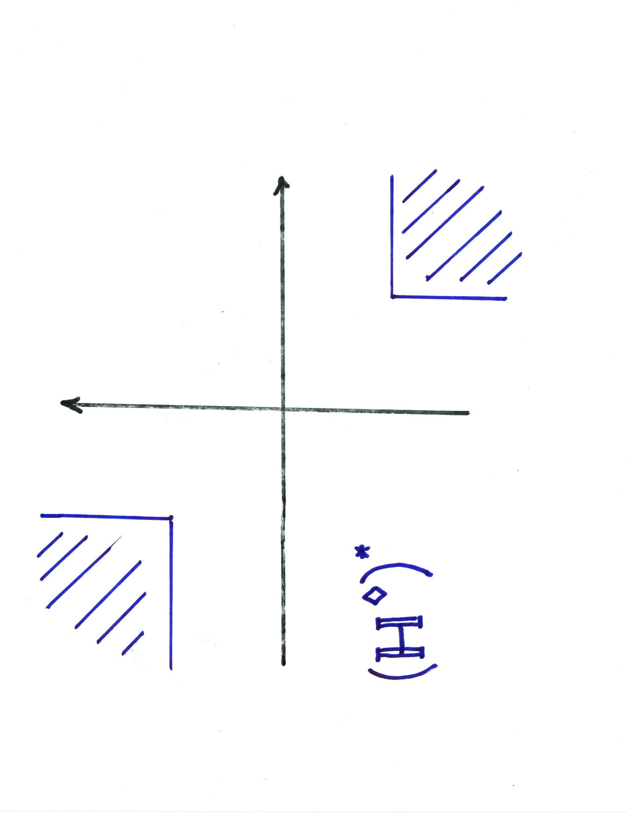 Figure 15
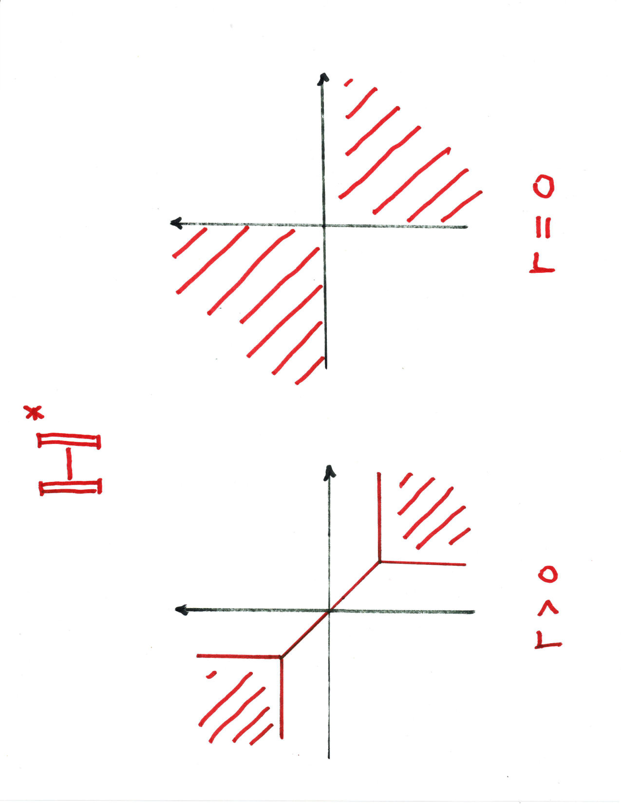 Figure 16
 Figure 2
 Figure 20
 Figure 21
 Figure 22
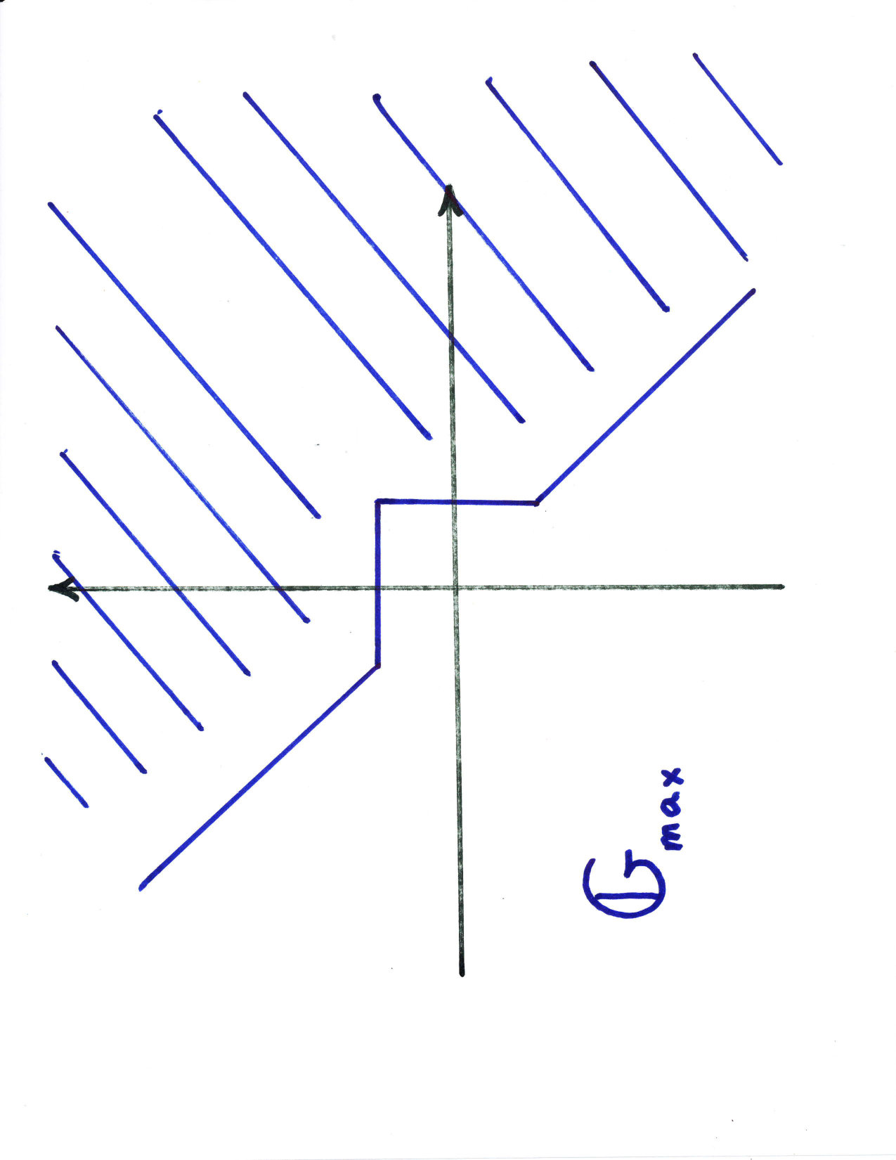 Figure 23
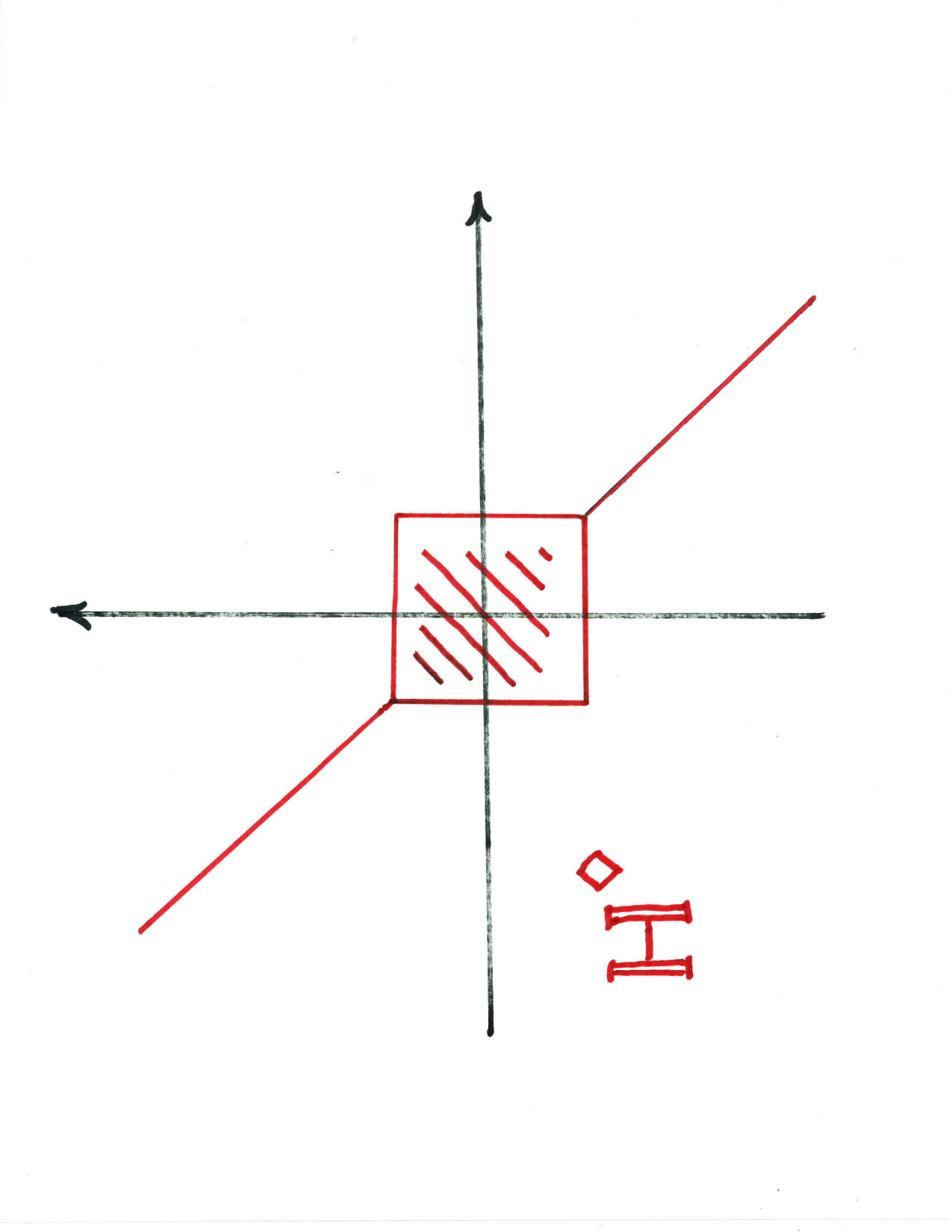 Figure 24
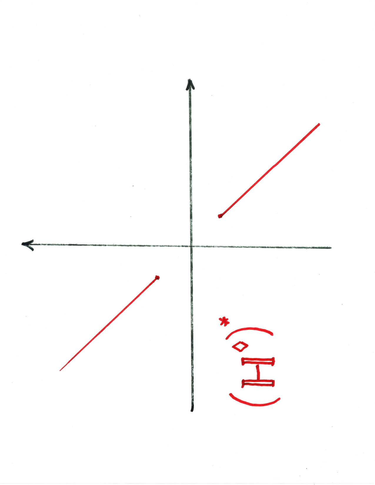 Figure 25
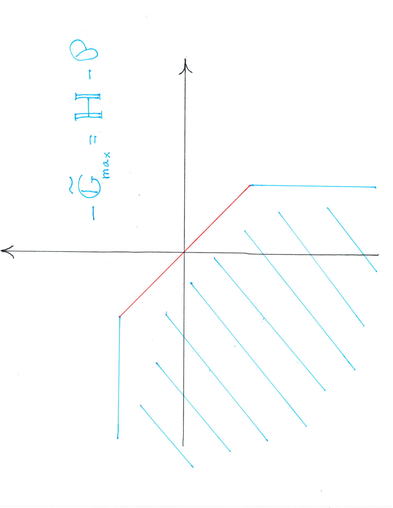 Figure 3
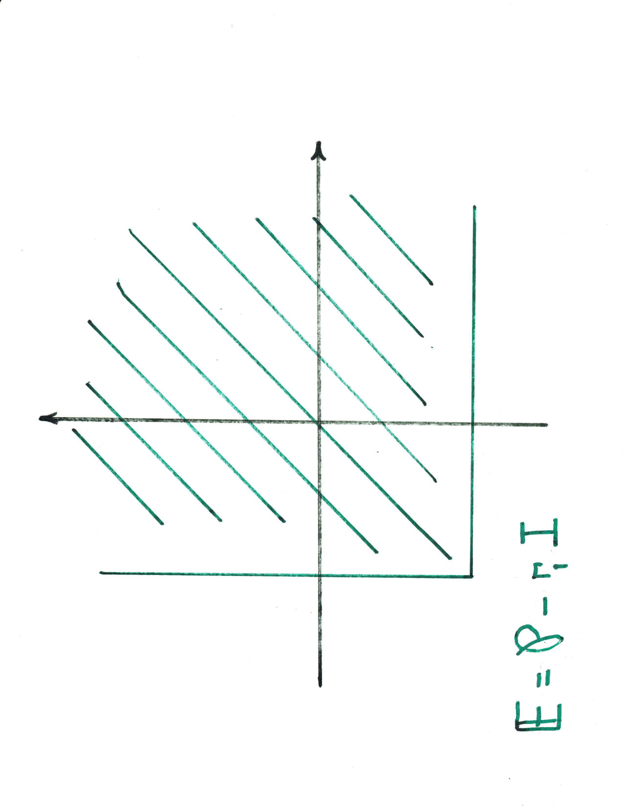 Figure 31
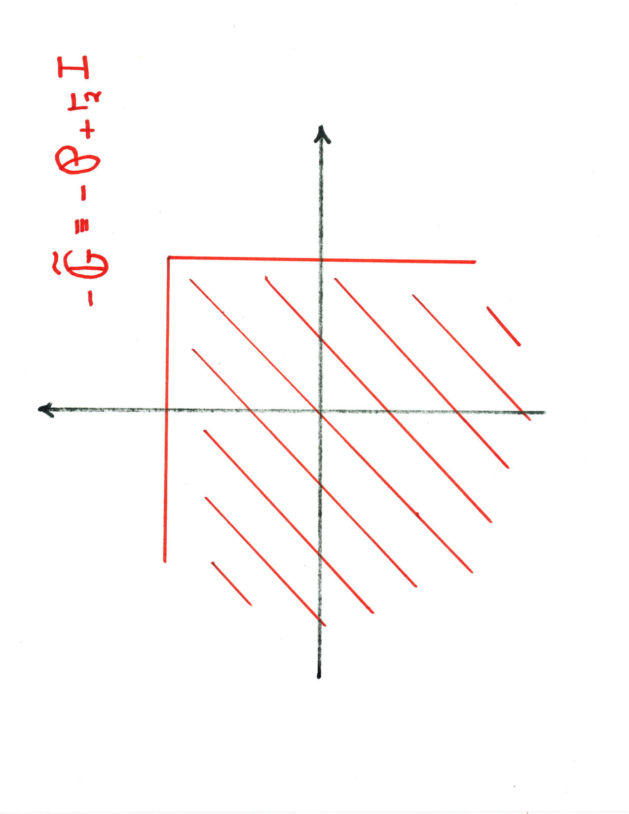 Figure 32
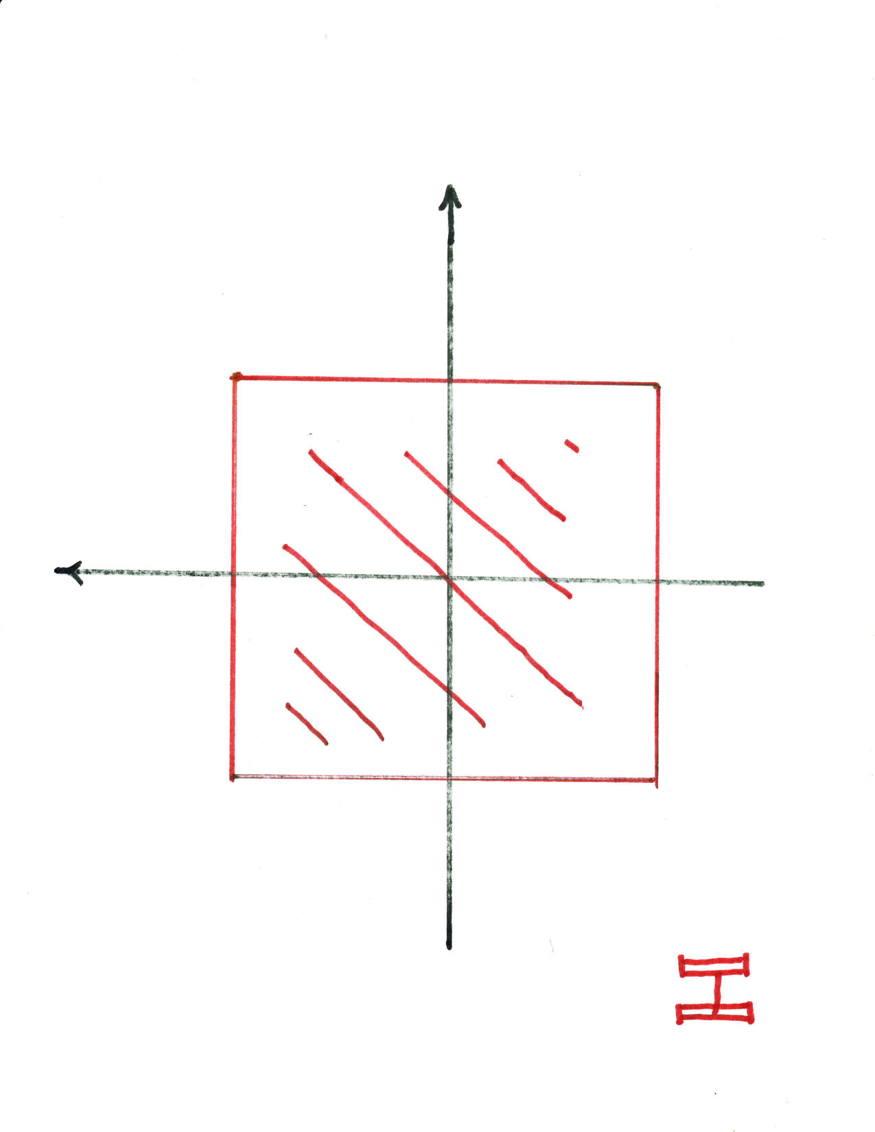 Figure 33
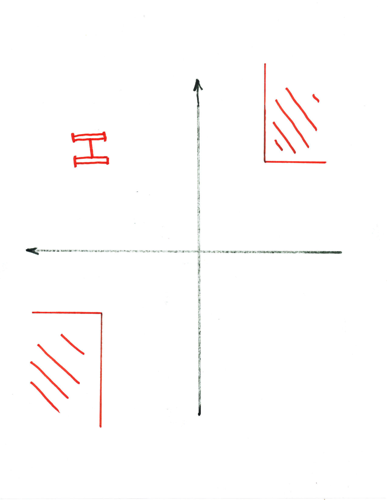 Figure 34
 Figure 4
 Figure 5
Peer Reviews
No public reviews on file for this paper yet. If you reviewed it on a platform where reviews are public (OpenReview, ICLR, NeurIPS, ICML), you can paste yours below so the community can read it here.
Videos
No videos yet. Explain this paper in a talk, walkthrough, or lecture? Add one.
A GENERALIZATION OF PDE’S FROM
A KRYLOV POINT OF VIEW
F. Reese Harvey and H. Blaine Lawson, Jr
Abstract.
We introduce and investigate the notion of a “generalized equation”, which extends nonlinear elliptic equations, and which is based on the notions of subequations and Dirichlet duality. Precisely, a subset is a generalized equation if it is an intersection where and are subequations and is the subequation dual to . We utilize a viscosity definition of “solution” to . The of is defined by . One of the main results (Theorem 2.6) concerns the Dirichlet problem on arbitrary bounded domains for solutions to with prescribed boundary function . We prove that:
(A) Uniqueness holds has no interior, and
(B) Existence holds has no interior.
For (B) the appropriate boundary convexity of must be assumed. Many examples of generalized equations are discussed, including the constrained Laplacian, the twisted Monge-Ampère equation, and the -equation.
The closed sets which can be written as generalized equations are intrinsically characterized. For such an the set of subequation pairs with is partially ordered (see (1.10)). If , then any solution for the first is also a solution for the second. Furthermore, in this ordered set there is a canonical least element, contained in all others.
A general form of the main theorem, which holds on any manifold, is also established.
Partially supported by the NSF
Table of Contents
-
Introduction
-
Main Definitions
-
The Canonical Pair Defining a Given ,
and an Intrinsic Characterization of Generalized Equations
-
Examples
-
Unsettling Questions
-
A General Case of the Main Theorem
Appendix A. The Quasi-Convexity Characterization of C1,1.
- Introduction.
For some time we have been studying fully nonlinear pde’s from a perspective of generalized potential theory. This was initiated by the discovery [6,7] of a robust potential theory attached to every calibrated manifold – a fact which generalized the classical pluripotential theory in Kähler geometry. Our point of view had some reflections in early work of Krylov [22], and eventually went far outside calibrated geometries. Good references for these techniques and results are [8], [9] and [10]
The purpose of this paper is to examine, to the fullest extent, when these viscosity and Dirichlet duality techniques can be employed to study nonlinear differential relations. Our fundamental Definition 2.2 is completely natural in the context of duality, but may seem to be too general or abstract. However, it turns out that there are lots of interesting examples: the constrained Laplace equation, the twisted Monge-Ampère equation, the relation in dimension 2, the -equation, and many, many more. Furthermore, our fundamental Theorem 2.6 gives a simple and somewhat surprising relationship with the two questions of existence and uniqueness.
For clarity and simplicity we restrict attention to the constant coefficient case until the last Section 6.
Before making more detailed comments about examples and results, we recall the fundamental background ideas.
Short Preliminaries
We adopt the subequation point of view from [8], [9], where a differential operator is replaced by the constraint set . (Here denotes the space of quadratic forms on .) The equation is replaced by the constraint condition . For that reason we will refer to as the equation associated to the subequation . The ellipticity hypothesis is assumed in the weakest possible form:
[TABLE]
Here . Any closed subset satisfying this positivity, or -monotonicty, condition (1.1), is called a subequation.111It is convenient occasionally in this paper to allow or .
The viscosity definition of a subsolution takes the following form. Consider an upper semi-continuous function defined on an open set and taking values in . An upper test function for at a point is a -function defined near with and . The function is said to be -subharmonic or an -subsolution on if for every upper test function at any point we have . For -functions , the consistency of this definition with the classical definition that for all , follows from the positivity condition (1.1). (In fact, consistency mandates positivity.) We will denote the space of -subharmonics functions on by . (For a complete introduction to viscosity theory see [2, 3].)
The Dirichlet dual of a subequation is defined to be
[TABLE]
It is also a subequation and provides a true duality . Moreover, one has the key relationship
[TABLE]
which enables one to replace by via the viscosity definitions (see Def. 2.1). It is easy to see that
[TABLE]
and to see that (1.1), together with being closed, implies the topological property
[TABLE]
(Also and are all path-connected.)
By (1.3) applied to , instead of , we have
[TABLE]
It is easy to see that
[TABLE]
and hence, by (1.6) we have
[TABLE]
This formula for the dual subequation could have replaced (1.2) as the definition of the dual subequation. It is frequently the easiest way to compute for examples, as in Section 4.
Generalized Equations
A generalized equation is simply a pair of subequations on . We associate to this pair the constraint set
[TABLE]
and define an -harmonic on an open to be a function on with
[TABLE]
i.e., is -subharmonic and is -subharmonic on . An -harmonic on which is satisfies the differential relation
[TABLE]
(by the consistency referred to above). One example is the constrained Laplacian (see Example 2.3 below)
[TABLE]
where and , i.e., . Here the -harmonics are classical harmonic functions with . This example can be generalized with being any closed subset of (see Example 4.3).
Another Example is the twisted Monge-Ampère Equation (Example 4.8) which has been studied by Streets, Tian and Warren, [24,25]. This equation requires a splitting of space, and uses a mixture of a convex and concave Monge Ampere operator on the two pieces. The authors proved an Evans-Krylov type estimate despite the nonconvexity of the operator. We are grateful for Jeff Streets communicating their work on this equation and asking us if any of our methods could apply.
A very nice example is given by taking and for . This is a special case of the quasi-convex/quasi-concave equation in Example 4.1. By a result of Hiriart-Urruty and Plazanet (which we present in Appendix A) we have
[TABLE]
Related to this is the quasi-subaffine/quasi-superaffine equation in Example 4.2. This equation is the mirror of the above. Let’s let and set . Then the intersection is another generalized equation (see Remark before (2.4)). The -harmonics of class satisfy
[TABLE]
A basic example is given by taking and , i.e., so that . This is a special case of the quasi-subaffine/quasi-superaffine equation in Example 4.2 (see also Example 4.16(d)). When , we see that .
When , we have and we are in the case discussed in the preliminaries above. Here there is no other pair giving the same .
Note however that a generalized equation can possibly be written as for many pairs of subequations . These pairs are partially ordered by saying
[TABLE]
If this holds, then any -harmonic on is automatically -harmonic on .
We shall see in Chapter 3 that for any generalized equation , there exits a unique canonical pair defining , which is all other pairs defining the set . Thus an -harmonic on , is harmonic for all pairs defining . It will be called a canonical -harmonic on . There remain some very interesting questions concerning this story (see Chapter 5).
One may wonder whether the closed sets which are generalized equations can be intrinsically characterized. They can be. They are exactly the sets satisfying:
[TABLE]
(See Theorem 3.5.)
Given this, it is natural to consider the canonical -harmonics on an open set . In Theorem 3.6 we show that if are generalized equations,
[TABLE]
Now whether or not a closed subset satisfies (1.11), the set
[TABLE]
is a generalized equation, and it is the smallest generalized equation containing . That is, it is contained in every other generalized equation containing . (See Theorem 3.7 for all of these facts.)
Recall that if . More generally, the negative of a generalized equation is also a generalized equation
[TABLE]
This might be viewed as the dual of a generalized equation.
More importantly, every generalized equation has a mirror, which is obtained by interchanging and . A shortened form of our main result is the following.
THEOREM 2.6. Suppose is a generalized equation with mirror , and that is a bounded domain. Then
[TABLE]
Suppose that is smooth and strictly and -convex. Then
[TABLE]
This allows us to divide generalized equations into four types depending on whether the interiors of and are empty or not. These types are strictly tied to the uniqueness and existence questions.
In proving Theorem 2.6 we established some results of independent interest.
Proposition 2.16. Fix boundary values . If there exist solutions to the -(DP) and to the -(DP) on , then . That is, is the common solution to the and the Dirichlet problems with boundary values .
Proposition 2.20. Assume uniqueness holds for , i.e., , for the generalized equation . Given a domain as above and , then:
[TABLE]
We would like to thank the referee for some very helpful suggestions.
- Main New Definitions and the Main Theorem.
To begin we discuss more completely the notion of a (determined) equation in the sense of [22], [8] and [9].
Definition 2.1. (Equation). A subset is a determined equation or just an equation if for some subequation . In this case a solution to the equation (or an -harmonic) on , is a function such that and .
Such functions are automatically continuous by definition. For -functions the consistency of this definition with the classical definition that for all , follows from (1.3) above that and the consistency property for subequations, mentioned in Section 1..
The main new concept in this paper is the following generalization.
Definition 2.2. (Generalized Equation). A subset is a generalized equation if
[TABLE]
for some pair of subequations . Just as in Definition 2.1 above, where , we define a solution to the (generalized) equation (or an -harmonic) to be a function with
[TABLE]
and let or denote the space of -solutions on .
As noted above, a generalized equation can possibly be written as for many pairs of subequations . These pairs are partially ordered by saying if and . If this holds, then any -harmonic on is automatically -harmonic on .
We present a guiding elementary example at this point to help the reader assimilate the many definitions presented here. Examples are discussed more fully in Section 4.
Example 2.3. (The Constrained Laplacian). Fix and let
[TABLE]
Define
[TABLE]
and note that since . We then define
Then we have
[TABLE]
with
We note that, with defined by as above, -harmonic implies -harmonic, which is of course obvious for -functions. This follows from Theorem 3.6 below. .
Remark. (Intersections of GE’s are GE’s). For general intersections of subequations and their negatives , we just get another generalized equation. The positivity condition (1.1) and the closure condition are both preserved under intersections. Hence and are subequations, and . (Also since and for subequations, one can show that .)
As before by definition such functions are continuous with the coherence property that if is , then
[TABLE]
For any generalized equation it is easy to see by (1.4) that the interior satisfies
[TABLE]
In particular,
[TABLE]
The Mirror
Each generalized equation has a mirror, which we now define.
Definition 2.4. (The Mirror Equation). If
[TABLE]
is a generalized equation, its mirror is defined to be the generalized equation
[TABLE]
In Example 2.3 we have since and are dual to one another.
This is a somewhat surprising example of a generalized equation from the following point of view. Consider and . By using viscosity theory in applying Definition 2.2 to , we have a notion of when has eigenvalues and , which differ in sign, for general continuous functions . Moreover, this is consistent with the classical definition if . On the other hand, there is nothing “elliptic” about a mixed sign constraint on . (The reader could also consider in Example 3.8 below where the eigenvalues also satisfy .)
Existence and Uniqueness
Examination of existence and uniqueness for the Dirichlet Problem for -harmonics leads to four distinct types of generalized equations, as follows.
Definition 2.5. Suppose is a bounded domain in . We say that existence for the (DP) for holds on if for all prescribed boundary functions there exists satisfying
(a) h\bigr{|}_{\Omega} is -harmonic, and
(b) h\bigr{|}_{\partial\Omega}=\varphi.
We say uniqueness for the (DP) for holds on if for all there exists at most one satisfying (a) and (b).
Now we can state our main result in this pure second-order constant coefficient case.
THEOREM 2.6. Suppose is a generalized equation with mirror , and that is a bounded domain. Then
[TABLE]
Suppose that is smooth and strictly and -convex. Then
[TABLE]
In fact, the following are equivalent:
(1) ,
(2) Uniqueness for the (DP) for holds on ,
(3) ,
(4) ,
and assuming that is smooth and both strictly and convex, these conditions are equivalent to
(5) Existence for the (DP) for holds on .
Interchanging with and with , we have the mirror list of equivalences:
(1)∗ ,
(2)∗ Uniqueness for the (DP) for holds on ,
(3)∗ ,
(4)∗ ,
and assuming that is smooth and both strictly and convex, these conditions are equivalent to
(5)∗ Existence for the (DP) for holds on .
Proof. It suffices to prove that (1) through (5) are equivalent because: (A) is just the statement that (2) (1), the mirror equivalences (1)∗ through (5)∗ are immediate from (1) through (5), and (B) is just the statement (1)∗ (5)∗.
Before proving the equivalence of (1) through (5) we list some trivial equivalences for any sets and .
Lemma 2.7. Suppose that and , then
[TABLE]
are equivalent. Interchanging and yields that
[TABLE]
are equivalent.
Proof. Note that obviously, since is an open subset contained in , by the hypothesis, follows from the definitions of the duals, and is trivial.
Corollary 2.8. If is a generalized equation with mirror , then
(1) is equivalent to (i) through (v), and
(1)∗ is equivalent to (i)∗ through (v)∗.
Proof. Note that (2.5) says that
[TABLE]
Hence, . Interchanging and yields .
Proof that (1) (3): By Corollary 2.8, (1) (i) which is (3).
Proof that (4) (1): If , then in particular which has no interior.
Proof that (1) (4): Note that and are disjoint unions. Hence, is the disjoint union of the four sets: , , , and . By (2.1) and (2.5), the last set , so that is the disjoint union of the three remaining sets. However, implies (3) and hence or . By Lemma 2.7 (iii) so that . Thus three of these four sets are empty leaving .
Proof that (1) (2): Recall from [9, Def. 8.1] the following form of comparison (C) for a subequation , which we will refer to as the zero maximum principle for sums, and abbreviate as either (ZMP for sums) or (C).
Definition 2.9. Given a relatively compact domain we say that comparison holds for on if for all upper semi-continuous functions on , with u\bigr{|}_{\Omega} -subharmonic and v\bigr{|}_{\Omega} -subharmonic, one has
[TABLE]
Comparison (C) always holds for pure second-order subequations and domains . This was first established in [8, Rmk. 4.9 and Thm. 6.4]. (See [1] for many other constant coefficient situations where comparison always holds. There are also some extensions in [9] to simply-connected, non-positively curved manifolds.) More precisely we have:
THEOREM 2.10. Suppose is a subequation and is a bounded domain. Then comparison (C) holds for on .
Now we can prove that (1) (2)
Proposition 2.11. Comparison (C) for both and on a domain implies that:
[TABLE]
Proof. By Corollary 2.8, . Therefore (C) for implies the (ZMP for sums) if is -subharmonic and is -subharmonic. If are two solutions to the -(DP) on with the same boundary values, then is –subharmonic and is –subharmonic on . Since on , the (ZMP) on . Interchanging and is possible since we are also assuming (C) for . This proves .
Proof that (2) (1):
Proposition 2.12. If there exists a function with for all , then uniqueness for the -(DP) on fails.
Proof. Take \varphi=h\bigr{|}_{\partial\Omega}. For any function , if is sufficiently small, we have for all . Thus the functions give many solutions to the Dirichlet problem with the same boundary values .
The following trivial fact is peculiar to the pure second-order, constant coefficient case (and the pure first-order case).
Lemma 2.13. Given any non-empty subset , there exists a function with for all .
Proof. Pick and take h(x)\equiv\hbox{{1\over 2}}\langle Ax,x\rangle so that for all .
Combining this Lemma with the previous Proposition proves the implication (2) (1) in the form:
[TABLE]
Next we treat the implication (1) (5) existence for the -(DP).
Proposition 2.14. If existence for the -(DP) holds on (Definition 2.6), then
[TABLE]
Proof. By Corollary 2.8 . Let denote the -harmonic function solving the (DP) with boundary values . Since is -subharmonic and , it is also -submarmonic. Since is -subharmonic, this proves that is -harmonic.
Recall the following from [8]. (As mentioned in §1, denotes the space of -subharmonic functions on .)
THEOREM 2.15. (Existence). Suppose has a smooth boundary which is both and strictly convex. Given , the Perron function h(x)\equiv\sup\{u\in{\rm USC}(\overline{\Omega}):u\in{\mathbb{E}}(\Omega)\ \ {\rm and}\ \ u\bigr{|}_{\partial\Omega}\leq\varphi\} solves the -(DP) on for boundary values .
Combining Proposition 2.14 with Theorem 2.15 yields
[TABLE]
on domains with strictly and convex smooth boundaries.
Before proving that (5) (1), or that implies non-existence for the -(DP), we need to establish some preliminary facts, which are also of independent interest.
Proposition 2.16. Fix boundary values . If there exist solutions to the -(DP) and to the -(DP) on , then . That is, is the common solution to the and the Dirichlet problems with boundary values .
Proof. By definition is -subharmonic and is -subharmonic on . Also, is -subharmonic and is -subharmonic on . Therefore,
[TABLE]
[TABLE]
Thus on .
Note: Then solves the generalized equation
[TABLE]
(One can show that . See [9, Property (2) after Def. 3.1] for arbitrary subsets of .)
Proposition 2.17. Recall again that comparison holds for and on . From this we conclude the following. If there exists a function with for all , then there is no solution to the -(DP) on with boundary values \varphi\equiv f\bigr{|}_{\partial\Omega}.
Proof. If exists, then since is an -solution, by Proposition 2.16 we have , and hence is . Thus . So this is impossible.
Proof that (5) (1) or that Non-Existence for . The fact that guarantees the existence of such a function by Lemma 2.13, and hence the non-existence for the Dirichlet problem.
This completes the proof of Theorem 2.6.
Four Types
In light of Theorem 2.6, if one is given a generalized equation with mirror , there are four distinct types possible which we label as follows.
Type I: and
Type II: and
Type III: and
Type IV: and
Note that Types I and II belong to part (A) of Theorem 2.6, and Types III and IV belong to part (B). We shall now discuss each type.
Type I: . This type is a “determined equation” as defined in Definition 2.1, because by (1) (3), and (1)∗ (3)∗, this is just the case where and are equal. We will call this subequation . Thus and are . Theorems 2.10 and 2.15 apply directly. Comparison holds for all bounded domains, and existence holds if is smooth and strictly and convex using results from [8].
Type II: and . Collecting together (1)–(5) and the negations of (1)∗–(5)∗ we have that
is a proper subset of and
Uniqueness but not existence holds for on any bounded domain . The opposite is true for , namely uniqueness for fails on all bounded domains , but if is smooth and both strictly and convex, then existence holds for on . In addition is a proper subset of both and . This is proven in (2.10) below.
For Type III we interchange with and with .
Type III: and . Collecting together (1)∗–(5)∗ and the negations of (1)–(5) we have that
is a proper subset of and
Uniqueness but not existence holds for on any bounded domain . The opposite is true for , namely uniqueness for fails on all bounded domains , but if is smooth and both strictly and convex, then existence holds for on . Also, is a proper subset of both and by (2.10).
Type IV: and . By (2.5) this is equivalent to
[TABLE]
Because of Lemma 2.7 (iii) and (iii)∗ this is equivalent to
[TABLE]
The main point here is that both existence and uniqueness for the (DP) for both and fail.
Next we consider the following.
Proposition 2.18. (Boundaries of Subequations). If is a determined equation, then the subequation with is uniquely determined by . In fact, is enough to conclude that for any two subequations and .
Proof. The first statement follows from (1.7) which holds for any subequation .
For the second statement note that one has . However, , but and . Hence, , and this implies that , which is equivalent to .
It follows that:
[TABLE]
Proof. If , then , so that by Proposition 2.18, and is Type I.
Next we begin to examine to what extent a generalized equation determines the subequations and . The answer in the determined case is given by next proposition. However, open questions concerning more general cases can be found is Chapter 5.
Proposition 2.19. (Uniqueness of the Defining Pair in the Determined Case). Suppose that where is a subequation. If for subequations and , then .
Proof. By (2.6) we have . By (2.5) we have . Therefore, , and so .
Now by (1.7) , and by the hypothesis , we have . Thus, . By the same hypothesis , we have . Hence by (1.8), , so that . This proves that .
The Question of Characterizing
the Boundary Functions for Existence
Here we turn to a natural question which arises in the Non-Existence cases, Types II and IV.
For which boundary functions
does there exists a solution to the -Dirichlet problem?
First we discuss the Type II case: Non-Existence/Uniqueness for . This is interesting, for example, for the constrained Laplacian above.
We make the assumption that is a bounded domain with smooth boundary which is both strictly and -convex. Using the equivalent versions (1)–(5) of the uniqueness hypothesis for in Theorem 2.6:
[TABLE]
this implies that is also strictly and -convex. Let denote the (unique) -harmonic function on with h_{\mathbb{E}}\bigr{|}_{\partial\Omega}=\varphi, and denote the (unique) -harmonic function on with h_{\mathbb{G}}\bigr{|}_{\partial\Omega}=\varphi. One answer to the question is the following.
Proposition 2.20. Assume uniqueness holds for , i.e., , for the generalized equation . Given a domain as above and , then:
[TABLE]
Proof. Suppose that and set . Then h\bigr{|}_{\partial\Omega}=\varphi, is -subharmonic, and is -subharmonic on , which proves that is a solution to the Dirichlet Problem (DP) on with boundary values .
Conversely, if these exists such an , then also solves the (DP) since is -subharmonic and is -subharmonic. Hence, . Similarly, since is -subharmonic and is -subharmonic.
The question posed above can also be asked in the Type IV case. It is intriguing for the “-equation” in Example 4.2 below. Here we take , and ask the question: How do we characterize the functions on the boundary of a domain which have a -extension with Lipschitz constant to all of ? This is related to Glaeser-Whitney extensions, for which there is a very large literature. The interested reader could consult [23], [4] for results and some history.
We finish this section with a general comment.
Remark 2.21. (Nice Properties of Generalized Equations). Recall that generalized equations are preserved under:
(1) Taking the mirror,
(2) Taking Intersections (see Remark before (2.4)),
(3) Taking the negative (see (1.13) ).
- The Canonical Pair Defining a Given , and an Intrinsic Characterization of Generalized Equations.
In this section we look at the question of which closed subsets of are generalized equations, and we characterize them. We start with the following.
Lemma 3.1. Suppose is any closed subset. Then
[TABLE]
is a subequation containing , and it is minimal with respect to these properties, i.e., if is any other subequation containing , then .
Proof. The set obviously satisfies positivity and so does its closure . To see this, let and choose a sequence with and . Now note that for all , .
Corollary 3.2. The set is the minimal subequation containing . Let
[TABLE]
Then denotes its dual .
Example. Let , where are the ordered eigenvalues of . Then is not closed. Nor is closed.
At the moment we do not have an example of this sort with a generalized equation.
Although it is only in the determined case that uniquely determines the defining pair (namely, ), we always have the following.
Proposition 3.3. (The Canonical Pair). Suppose is any generalized equation. Then there exists a canonical choice for the subequation pair defining , namely and :
[TABLE]
This canonical pair is characterized by the following property:
If is any other subequation pair yielding the same generalized equation , i.e., if then
[TABLE]
i.e., is minimal and is maximal.
In particular, if is harmonic for the canonical min/max pair , then is also harmonic for all other pairs .
Proof. Since and , we have that
[TABLE]
Now assume that for a subequation pair . Then and so . We also have which implies that . Thus we have and . Therefore, . With the display above, this implies that .
The next result concerns a generalized equation belonging to part (A) of Theorem 2.6 – the uniqueness case. This is the case where , or equivalently by Theorem 2.6, this is the case of a generalized equation which is either of Type I or Type II. Given a generalized equation , another characterization is
[TABLE]
(This follows easily from Theorem 2.6.)
Proposition 3.4. Suppose is a generalized equation with (that is, belongs to part (A) of Theorem 2.6 – the uniqueness case). Let denote the canonical min/max pair with . Any subequation with must satisfy
[TABLE]
Proof. Note that . Now . Hence, .
One may wonder whether the closed sets , which are generalized equations, can be intrinsically characterized. They can be.
THEOREM 3.5. (The Characterization of Generalized Equations). A closed subset is a generalized equation if and only if
[TABLE]
Proof. First, by (3.3) this equation holds for any generalized equation .
For the converse, recall from Lemma 3.1 that the sets and are always subequations, so that is a generalized equation.
As we have seen, if is a generalized equation then the set of pairs with is partially ordered with a unique minimal element . So associated to we have this canonical subequation pair , and it is natural to consider the associated canonical -harmonics.
THEOREM 3.6. Let be two generalized equations as in Theorem 3.5. Then any function which is -harmonic on an open set is also -harmonic on .
Proof. We shall use the second form of (3.3). Note that and . Therefore, , and which means that . Thus if is -subharmonic and is -subharmonic, this also holds for the primed subequations.
This theorem says that the partial ordering by inclusion on the family of closed subsets which are subequations, carries over to their canonical harmonics on any open . The reader will also recall that a canonical -harmonic on is also an -harmonic for any other pair with . One could certainly wonder whether every -harmonic is canonically -harmonic. (This is discussed as the “Broadened Equation Question” in Section 5.) If this were true, the theory would be very tidy.
THEOREM 3.7. (The GE Associated to a Closed Set). Let be any closed subset. Then the pair of subequations
[TABLE]
gives a generalized equation
[TABLE]
containing , and it is the smallest such. That is, if is a subequation pair with , then . Moreover, is the canonical min/max pair defining .
More succinctly, every closed subset gives rise to a minimal generalized equation containing , namely
[TABLE]
Proof. From Lemma 3.1 and Corollary 3.2 we know that is a pair of subequations defining the generalized equation given in (3.6), which clearly contains .
Suppose are subequations with . Then and so . Also , so and therefore . Hence, as claimed. Finally, {\mathbb{E}}_{\rm min}\buildrel{\rm def}\over{=}(\overline{{\mathbb{H}}^{\diamondsuit}+{\mathcal{P}}})\supset(\overline{{\mathbb{H}}+{\mathcal{P}}})\buildrel{\rm def}\over{=}{\mathbb{E}}^{\diamondsuit} (since ), and implies , which proves . The proof that , so that , is similar.
Example 3.8. Let
[TABLE]
Then
[TABLE]
Therefore, the minimal generalized equation containing is
[TABLE]
Note that the canonical pair for this generalized equation is:
[TABLE]
Some Facts: Here and are dual to one another, and so
[TABLE]
is a Class II generalized equation (see Section 4).
The mirror of is
[TABLE]
Both and , so that is Type IV.
Example 3.9. Let
[TABLE]
Then we have
[TABLE]
Therefore, the minimal generalized equation containing is
[TABLE]
Note that the two subequations are:
[TABLE]
Some Facts: Here and are dual to one another, and so
[TABLE]
is a Class II generalized equation (see Section 4).
The mirror of is
[TABLE]
Here we have and , so that is Type III.
- Examples of Generalized Equations .
We start with some classes of examples. First and foremost is the following.
Class I. Type I Determined Equations (The Case). Here is the boundary of a subequation . We refer to [8], [9] and [10] for an abundance of important specific examples.
Another important class of examples is
Class II. (The Case). Here and . Note that the overlap between Classes I and II consists of the boundaries of self-dual subequations (where the dual equals ).
Class IIa. (Edges). In this Class II, the most basic examples are when is a convex cone subequation. Then is a vector subspace called the edge of the cone . Since is a proper subspace, is also a proper subspace, and hence . Now note that is false for a proper convex cone because is an open convex cone. Equivalently, is false. By the equivalence of (1)* and (3)* in Theorem 2.6, this proves that . Thus is Type II. Such edge harmonics include: (i) Affine functions, where and , (ii) pluriharmonic functions in complex analysis, where and the edge is SkewHerm, (iii) -harmonic functions, and many others. The “edge” generalized equations are the subject of [19].
Three specific non-edge Class II examples are as follows.
Some Non-Uniqueness Examples
Example 4.1. (The Quasi-convex/Quasi-concave Equation) Choose with , and let
[TABLE]
Here is the subequation for -quasiconvex functions, and is the subequation for -quasiconvex functions. Thus is the generalized equation for functions that are both -quasiconvex and -quasiconcave. Note that . A function is -harmonic is convex and is concave.
Observe now that if satisfies this generalized equation, then the function satisfies the generalized equation. Thus, by simply adding multiples of we translate the equation up and down the line . So we can assume that , in fact let’s assume . In this case and is class II above, and Type IV. Furthermore, there is the following result of Hiriart-Urruty and Plazanet in [20]. An alternate proof appeared in [5]. For the benefit of the reader we include a proof in Appendix A.
We say that a function is if it is and the first derivative is Lipschitz with Lipschitz coefficient .
THEOREM A.1. For a function on a convex domain ,
[TABLE]
Here is a related example which produces the mirror equation to the one above.
Example 4.2. (The Quasi-subaffine/Quasi-superaffine Equation). Choose and set
[TABLE]
Here is the subequation for -quasi-subaffine functions, i.e., is subaffine, and is again the subequation for -quasi-subaffine functions. Again if , then and is a special case of Class II above.
If , then consider and in Example 4.1. Then here in Example 4.2, the subequation is equal to . Thus the mirror of in Example 4.1 is in Example 4.2.
The Intersection of Examples 4.1 and 4.2. From Example 4.1 we have
[TABLE]
[TABLE]
Recall that the GE in Example 4.2 is just the mirror where
[TABLE]
Hence we have
[TABLE]
The -harmonics for this GE are ’s with and . This can be expressed invariantly as
[TABLE]
or in keeping with the Twisted Monge-Ampère Example 4.8
[TABLE]
Note: There are lots of such harmonics. For example,
[TABLE]
Some Type II Examples of Non-Existence and Uniqueness for
Example 4.3. (Generalized Constrained Laplacians).
Definition 4.4. A closed subset of (with ) will be called a (generalized) constrained Laplacian.
Lemma 4.5. If is a (generalized) constrained Laplacian, then is closed and hence a subequation. Furthermore, is closed, and
[TABLE]
so that is a generalized equation with and .
Proof. Suppose , i.e., with and . Set . Since , we have . Thus . The set with is compact. Therefore we can extract a convergent subsequence of , which we again call , with . Therefore, . Since is closed and each , we have . Thus with and , and so we have proved that is closed. Replacing by we have that is closed. Thus is closed.
Obviously . Suppose now that , i.e., for and . Then . Since , this implies that , and hence .
Note that , so must be type I or type II. However, it cannot be type I without (cf. Propositions 2.18 and 2.19). This proves
[TABLE]
Question 4.6. Suppose and define and is a generalized constrained Laplacian. If is -harmonic, then is -harmonic?
Example 4.7. Let and
[TABLE]
with . Then
[TABLE]
One could also look at this from the universal eigenvalue point of view (see the subsection of Section 5 in [11] and Remark 4.12 below), by taking the eigenvalues of and . Let denote the positive orphant defined by for all , and let be similar with coordinates . Then can be defined by
[TABLE]
[TABLE]
[TABLE]
A great example of a non-existence/uniqueness equation (Type II) has been introduced and studied in [24] and [25]. This is discussed next.
Example 4.8. (The Universal Version of the Twisted Monge-Ampère Equation). The real twisted Monge-Ampère equation is defined by consisting of all
[TABLE]
i.e., , or .
As in Example 4.7, the universal version of this equation is defined on by
[TABLE]
Lemma 4.9. Let . Then is fibred over , where the fibre of at is the dual MA universal subequation:
[TABLE]
Since it is easy to see that is closed, is equal to the minimal subequation defined above for this .
Proof of Lemma 4.9. First note that is fibred over with fibre at given by
[TABLE]
Second note that this equals
[TABLE]
the boundary of the dual MA-subequation at level . Third note that, since is a subequation,
[TABLE]
Defining by its fibres over , we have , and it remains to show . But , so it is emough to show is -monotone. As noted above is -monotone since is a subequation. Now increasing one of the coordinates with increases proving that is -monotone. Finally the orphant equals the product .
Lemma 4.10. Let . Then is fibred over , where the fibre of at is the dual MA universal subequation:
[TABLE]
The proof of Lemma 4.10 is similar to the one for Lemma 4.9, and is skipped.
Proposition 4.11. is a universal version of a generalized equation with minimum subequation and maximum subequation .
Proof. Note that and by Lemma 4.9. Note also that
[TABLE]
by Lemma 4.10.
Now assume . Then or otherwise said, and . Also, or otherwise said, and .
In summary, if , then
[TABLE]
that is, . It is easy to see that .
Remark 4.12. (Universal Equations and Gårding/Dirichlet Operators). A closed subset which is symmetric under permutations of the coordinates and satisfies is called a universal eigenvalue subequation. There is an obvious one-to-one correspondence between subequations , which depend only on the eigenvalues of , and universal subequations . However, this is only one of many subequations determined by which are constructed by substituting Gårding eigenvalues for regular eigenvalues as follows.
Let be a homogeneous polynomial of degree , on some , which satisfies the conditions of being a Gårding/Dirichlet, or GD, operator (as defined in [11, §5]). Then for each this operator gives eigenvalues , and so determines a subequation in by:
[TABLE]
For example, the universal subequation determines the Gårding Monge Ampère subequation {\mathbb{F}}^{g}_{\Lambda}=\{A\in{\rm Sym}^{2}({\mathbb{R}}^{m}):\lambda_{g,1}(A),..,\lambda_{g,n}(A)\ \text{are all \geq 0}\}, which is just the closed Gårding cone for .
This carries over to generalized equations. A generalized universal equation is any closed which is an intersection involving two two universal subequations . For example, the universal Laplacian determines a Gårding Laplacian for each GD operator of degree . Moreover, given a pair of GD operators of degrees , one has a constrained Laplacian generalized equation induced by the universal version of the constrained Laplacian given in Example 2.3. Namely, we have
[TABLE]
Example 4.13. (Twisted Gårding MA Generalized Equations). Similarly (we leave this to the reader) the universal twisted MA-equation (Example 4.8) spawns a huge family of generalized equations. For instance, in addition to the real version in [24], [25], one has a complex version, a quaternionic version, a Lagrangian version, branched versions of these three, elementary symmetric versions of these three (the so-called “hessian equation” versions), just to name a few.
The Examples 4.1 and 4.2 can also be viewed as “universal subequations”, spawning many more examples of generalized equations as above.
Since we have no reason to rule out or as a subequation in this paper, we have that equal to plus or minus a subequation is an example of a generalized equation of Type III or II respectively.
Example 4.14. (Subequations as Generalized Equations). For any subequation , if we choose , i.e., , then is a generalized equation. Now since and , we have . Also the mirror . Hence, . In summary, if is any subequation, then with , we have and , so that itself (not ) is a generalized equation which falls in the Existence/Non-Uniqueness case for (Type III). Similarly, with and is Type II.
Some Type IV Examples of Non-Uniqueness/Non-Existence.
Example 4.15. With coordinates , define by and by (so that is the subaffine subequation on considered as a subequation on ). Then with we have that the -harmonics are continuous functions that are separately convex in and concave in . The mirror -harmonics are continuous functions that are separately subaffine in and superaffine in .
Elementary Examples from and
Example 4.16.
(a) If we take , then is the determined equation whose harmonics are solutions to the real Monge-Ampère equation.
(b) If we take , then is the determined subaffine equation, whose harmonics are the negatives of the harmonics for real Monge-Ampère equation.
(c) If we take and , then , and the harmonics are functions which are both convex and concave, i.e., the affine functions. So far nothing is really new.
(d) If we take and , then . The solutions are functions with non-definite, (i.e., never nor ) in the case.
The Affine Generalized Equation
Example 4.17. Here we are interested in equations where . Note that . Therefore
[TABLE]
Proposition 4.18. Suppose is a convex cone and let be its polar cone.
Suppose (equivalently )
such that (equivalently ). Then is -harmonic is -harmonic is affine.
Proof. is -harmonic is subharmonic and is subharmonic. Therefore, is -harmonic is -harmonic is smooth is affine.
Proposition 4.19. Any affine generalized equation is Type II, i.e., and .
Proof. Of course . Now , which proves that is Type I. Hence and so . This is impossible for a subequation , so .
Recall for Type II that .
The canonical pair for is given as follows.
.
We have .
In this case an harmonic is affine since are both convex.
- Unsettling Questions.
In Section 8 of [18] we posed several such questions, starting with the single-valuedness of operators and the following equivalent restatement of that question.
(CCQuest) Constant Coefficient Subequation Question: Can a pair of subequations , with disjoint equations, i.e., , have a simultaneous harmonic ?
Of course a simultaneous harmonic cannot be since one would have . One reason for the success of viscosity theory is that the intuition gained from examining classical situations carries over to the viscosity approach. In fact, one can show that any simultaneous harmonic must be quite bizarre, but this is short of non-existence. (A known result which has some kinship to this open question is the fact that an arbitrary upper semi-continuous function has an upper test function at a dense set of points, cf. [13, Lemma 6.1*′*].)
In this section we first discuss some equivalent versions of the question above. We then examine an extension of this question to a natural one for any generalized equation.
It is easy to see from positivity that the boundary of a subequation can be expressed as the graph of a continuous function over the hyperplane . Consequently, if , we might as well assume . Now the hypothesis of (CCQuest) can be reformulated as follows.
[TABLE]
We leave the proof to the reader. The condition in (5.1a) is obviously equivalent to:
[TABLE]
Lemma 5.1. Under the equivalent assumptions of (5.1)
[TABLE]
Proof. First suppose is -harmonic, i.e., is -subharmonic and is -subharmonic. By (5.1) and hence also. Thus is both and subharmonic and is both and subharmonic, which proves that is both and harmonic.
For the converse suppose that is both and harmonic. Then is subharmonic and is -subharmonic, so that is -harmonic.
This equivalence (5.2) means that we can reformulate the above (CCQuest) concerning simultaneous harmonics for and as follows.
(CCQuest)′: Does there exist a subequation pair defining the generalized empty equation with the property that has a harmonic?
Summary. There are lots of subequations pairs defining this generalized empty equation . For some of these pairs we can prove that has no harmonics. For example, this holds if -harmonics and -harmonics are always because of Lemma 5.1. To conclude we note that for the canonical defining pair is , so that for this pair defining there are also no harmonics.
Now we can broaden our question as follows.
Broadened Equation Question: Given a generalized equation does there exists a subequation pair defining so that has a harmonic which is not a harmonic for ?
Note that by Proposition 3.1 and so that harmonics are always harmonics.
As for (CCQuest), any such harmonic in this Broadened Equation Question must be weird and pathological, much worse than for sure.
- The General Case of the Main Theorem.
For clarity and simplicity we have been restricting attention to pure second-order constant coefficient subequations and to define a generalized equation in . However, the main Theorem 2.6 holds for completely general subequations on manifolds, as defined in [9], and we give that result in this section. For general definitions we refer to [9]. However, there are many interesting cases which the reader could keep in mind (without consulting [9]), namely: constant coefficient subequations and (not necessarily pure second-order) in , variable coefficient subequations (constraint sets for subsolutions) on domains in , subequations on riemannian manifolds given canonically by O()-invariant equations in , subequations on hermitian manifolds given canonically by U()-invariant equations in , etc.
Let be the 2-jet bundle on a manifold . (When this is just the bundle over of order-2 Taylor expansions.)
THEOREM 6.1 Let be a domain in a manifold , and suppose are two subequations. Consider the generalized equation .
(a) uniqueness for the -(DP) on , assuming that comparison holds for and on .
(b) existence holds for the -(DP) on , assuming that existence for the -(DP) holds on .
(c) There exists with for all non-uniqueness for the -(DP) on for the boundary values \varphi\equiv h\bigr{|}_{\partial\Omega}.
(d) There exists with for all non-existence for the -(DP) on for the boundary values \varphi\equiv f\bigr{|}_{\partial\Omega}, assuming that comparison holds for and on .
Proof of Assertion (a). We begin by noting that assertions (1.2) – (1.5) hold for general subequations as defined in [9]. Our definition of is the same as in Definition 2.2, and the assertion (2.5) carries over. As a result, Lemma 2.7 and Corollary 2.8 hold in this general case. We now look at the proof of Proposition 2.11, which carries over and says that under the assumption of comparison (C) for both and we have Part (a).
Proof of Assertion (c). This follows exactly the argument given for Proposition 2.12.
Proof of Assertion (b). This follows exactly the argument given for Proposition 2.14.
Proof of Assertion (d). We are assuming that comparison (C) holds on for both and . This means that Proposition 2.16 holds, and therefore also Proposition 2.17 is valid. This establishes Part (d).
Example 6.2. (Generalized Constant Coefficient Equations in ). Here a subequation is, by definition (cf. [9], [10]), a closed subset
[TABLE]
such that for and and such that . The topological condition was not part of our definition of a subequation in Section 1, which was for pure second-order subequations. This allowed us to use the simpler definition that is closed, since then follows easily from the positivity condition (1.1).
With regards to Assertion (a) comparison does not hold for all such equations. However it does hold for many interesting classes, for instance, all gradient free ones. Other such classes can be found in [1].
On the other hand, existence does hold for all these equations , under the hypothesis that the domain has a smooth strictly and convex boundary. (See Theorem 12.7 in [9].) Now in Assertion (b) existence is only required for . Therefore, Assertion (b) holds for provided is strictly and convex.
Example 6.3. (Generalized Equations on an open set ). The general subequation here is a closed subset of the 2-jet bundle
[TABLE]
such that
[TABLE]
, and for the fibres we have
[TABLE]
These are barebones hypotheses needed for the constraint set for subsolutions of a nonlinear equation corresponding to .
This is the general case for domains , and so the comparison and existence hypotheses in Theorem 6.1 need to be verified, but, of course, the literature is enormous.
For subequations on manifolds given by “universal” equations, much has been done in [9]. We shall now look at some cases.
Example 6.4. (Universal Subequations Defined on any Riemannian Manifold). Let be a subequation (as in Example 6.2) which is invariant under the natural action of the orthogonal group O (or SO). Then determines an invariant subequation on any riemannian (or oriented riemannian) manifold as follows.
Every -function on has a riemannian hessian , which is a section of the bundle of symmetric 2-forms on , given at by
[TABLE]
where is the Levi-Civita connection on . Note that , so the symmetry and the tensorial properties of follow.
Now this riemannian Hessian gives a splitting of the 2-jet bundle
[TABLE]
and the orthogonally invariant subequation canonically determines a subequation as follows. Any orthonormal frame field for on an open set determines an orthonormal framing of . Via this framing, determines a subequation on . However, if we use a different frame field , the two framings of differ pointwise by O-transforms. By the O-invariance of the subequation on are the same. This also means that on two different open sets the two subequations agree on . Hence, we have a well-defined global subequation .
For example, if , we get the subequation for the riemannian Laplacian. If , we get the real Monge-Ampère subequation . If , one gets the infinite Laplacian on .
The questions of comparison and of existence of solutions for the Dirichlet problem on manifolds are addressed in [9]. A cone subequation on is a cone monotonicity subequation for if . Then for such equations we have the following from Thm. 13.2 and Thm. 10.1 in [9]. (See section 14 of [9] for examples.)
THEOREM ([9]). Suppose admits a strictly -subharmonic function. Then comparison for holds on any domain , and if is smooth and strictly and convex, then existence holds for the Dirichlet problem for all boundary functions .
This construction has important generalizations.
Example 6.5. (Universal Subequations Defined on a Riemannian Manifold with -Structure). We now assume that the riemannian manifold can be covered by open sets , with an orthogonal tangent frame field on , such that on the intersection of two such, the change of frames from to always lies in a given compact subgroup .
For example, if has an orthogonal almost complex structure , then has an U-structure.
If the euclidean subequation is -invariant, then the above construction gives a canonical subequation on any riemannian manifold with -structure. For example, for above, we can define the complex Monge-Ampère operator.
The Theorem at the end of Example 6.4 extends to these cases.
Example 6.6. (Geometric Cases). Of particular importance are the geometric cases given by a closed subset of the Grassmannian of -planes in . We assume that {{\bf G\!\!\!\!l}}\ is invariant under a closed subgroup . Then we consider the universal euclidean subequation
[TABLE]
This subequation now carries over to any riemannian manifold with -structure. For instance, suppose {{\bf G\!\!\!\!l}}\ is the set of special Lagrangian -planes in . Then we get a subequation on any Calabi-Yau manifold . If {{\bf G\!\!\!\!l}}\ is the set of associative 3-planes in , then we get a subequation on any 7-manifold with holonomy .
Theorems in [9] apply to these cases, but there is a better theorem in [12]. We define the {{\bf G\!\!\!\!l}}\-core of to be the set
[TABLE]
THEOREM ([12, Thm. 7.6 and Thm. 7.7]). If , then comparison for holds on any domain , and if is smooth and strictly {\mathbb{F}}_{{\bf G\!\!\!\!l}}\ and convex, then existence holds for the Dirichlet problem for all boundary functions .
Remark 6.7. In Section 2 we made a remark which does not carry over to general subequations. Finite intersections of subequations are not always subequations. There are classes of subequations where this is true (see [1]). However in general this means that one could expand the definition of a generalized equation to cover many-fold intersections and unions of subequations. This will be done elsewhere.
Appendix A. The Quasi-Convexity Characterization of C1,1.
Interestingly, the condition that a function be locally is equivalent to locally being simultaneously quasi-convex and quasi-concave. This was probably first observed by Hiriart-Urruty and Plazanet in [20]. An alternate proof appeared in Eberhard [5] and also in [21]. For the benefit of the reader we include a proof here.
We say that a function is if it is and the first derivative is locally Lipschitz with Lipschitz coefficient .
THEOREM A.1.
[TABLE]
Proof. We consider on a convex set .
() Suppose that is -, i.e., and for all . Set . Then
[TABLE]
and hence
[TABLE]
This form of monotonicity of is one of the standard definitions of being convex. The same proof works for
( ) We state the converse as a proposition.
Proposition A.2. If and are -quasi-convex on a convex domain , then and
[TABLE]
Proof. We first show that this is true if . Note that are -quasi-convex and for all for all . Fix . By the Mean Value Inequality in [26], for some , and hence . (Here is the operator norm of the symmetric transformation , which is equal to the max of over unit vectors .)
In general, since the graph of has a supporting hyperplane from below and the graph of has a supporting hyperplane from above, at every point, the function is differentiable everywhere. By partial continuity of the first derivative for quasi-convex functions (see for example Lemma 1.3 in [13]), we have .
Now standard convolution works just fine to complete the proof since is -quasi-convex by the next lemma, and the fact that locally uniformly.
Lemma A.3. is -quasi-convex is -quasi-convex.
Proof. Suppose is -quasi-convex, i.e., is convex. Standard convolution of with an approximate identity based on (i.e., ) yields smooth and convex. Note that preserves modulo an affine function, since where and . Therefore, , proving that each is -quasi-convex.
REFERENCES
[1] M. Cirant, F. R. Harvey, H. B. Lawson, Jr. and K. R. Payne, Comparison principles by monotonicity and duality for constant coefficient nonlinear potential theory and pde’s.
[2] M. G. Crandall, H. Ishii and P. L. Lions User’s guide to viscosity solutions of second order partial differential equations, Bull. Amer. Math. Soc. (N. S.) 27 (1992), 1-67.
[3] M. G. Crandall, Viscosity solutions: a primer, pp. 1-43 in “Viscosity Solutions and Applications” Ed.’s Dolcetta and Lions, SLNM 1660, Springer Press, New York, 1997.
[4] A. Daniilidis, M. Haddou, E. Le Gruyer, and O. Ley, Explicit formulas for Glaesner-Whitney extensions of 1-Taylor fields in Hilbert spaces, Proc. A. M. S., 146, no. 10 (2018), 4487-4495.
[5] A. Eberhard, Prox-regularity and subjets, in: A. Rubinov (Ed.), Optimization and Related Topics , Applied Optimization Volumes, Kluwer Academic Publishers, Dordrecht, 2001, pp. 237-313.
[6] F. R. Harvey and H. B. Lawson, Jr, An introduction to potential theory in calibrated geometry, Amer. J. Math. 131 no. 4 (2009), 893-944. ArXiv:math.0710.3920.
[7] ———– , Duality of positive currents and plurisubharmonic functions in calibrated geometry, Amer. J. Math. 131 no. 5 (2009), 1211-1240. ArXiv:math.0710.3921.
[8] ———– , Dirichlet duality and the non-linear Dirichlet problem, Comm. on Pure and Applied Math. 62 (2009), 396-443.
[9] ———– , Dirichlet duality and the non-linear Dirichlet problem on Riemannian manifolds, J. Diff. Geom. 88 No. 3 (2011), 395-482. ArXiv:0907.1981.
[10] ———– , Existence, uniqueness and removable singularities for nonlinear partial differential equations in geometry, pp. 102-156 in “Surveys in Differential Geometry 2013”, vol. 18, H.-D. Cao and S.-T. Yau eds., International Press, Somerville, MA, 2013. ArXiv:1303.1117.
[11] ———– , Hyperbolic polynomials and the Dirichlet problem, ArXiv:0912.5220.
[12] ———– , Geometric plurisubharmonicity and convexity - an introduction, Advances in Math. 230 (2012), 2428-2456. ArXiv:1111.3875.
[13] ———, Notes on the differentiation of quasi-convex functions, ArXiv:1309.1772.
[14] ———– , Gårding’s theory of hyperbolic polynomials, Communications in Pure and Applied Mathematics 66 no. 7 (2013), 1102-1128.
[15] ———– , Potential theory on almost complex manifolds, Ann. Inst. Fourier, Vol. 65 no. 1 (2015), p. 171-210. ArXiv:1107.2584.
[16] ———– , Lagrangian potential theory and a Lagrangian equation of Monge-Ampère type. ArXiv:1712.03525.
[17] ———– , Characterizing the strong maximum principle for constant coefficient subequations, Rendiconti di Matematica 37 (2016), 63-104. ArXiv:1303.1738.
[18] ———– , The inhomogeneous Dirichlet problem for natural operators on manifolds. ArXiv:1805.11121.
[19] ———– , Pluriharmonics in general potential theories. ArXiv:1712.03447.
[20] J.-B. Hiriart-Urruty, Ph. Plazanet, Moreau s Theorem revisited, Analyse Nonlinéaire (Perpignan, 1987), Ann. Inst. H. Poincaré 6 (1989), 325-338.
[21] J.-B. Hiriart-Urruty, How to regularize a difference of convex functions, J. of Math. Anal. and Appls., 162 (1991), 196-209.
[22] N. V. Krylov, On the general notion of fully nonlinear second-order elliptic equations, Trans. Amer. Math. Soc. 347 (1995), 857-895.
[23] E. Le Gruyer, Minimal Lipschitz extensions to differentiable functions defined on a Hilbert space, Geom. Funct. Anal. 19 (2009), no. 4, 1101 1118.
[24] J. Streets and G. Tian, A parabolic flow of pluriclosed metrics, Int. Math. Res. Not. 16 (2010), 3101-3133.
[25] J. Streets and M. Warren, Evans-Krylov estimates for a non-convex Monge-Ampère equation, ArXiv:1410.2911.
[26] W, Rudin, Principles of Mathematical Analysis, McGraw-Hill, New York, NY, 1953.