B-spline-like bases for C2 cubics on the Powell-Sabin 12-split
\firstnameTom \lastnameLyche
University of Oslo, Department of Mathematics, P.O. Box 1053, Blindern, NO-0316, Oslo, Norway
[email protected]
and
\firstnameGeorg \lastnameMuntingh
SINTEF Digital, Department of Mathematics and Cybernetics, P.O. Box 124 Blindern, NO-0314, Oslo, Norway
[email protected]
Abstract.
For spaces of constant, linear, and quadratic splines of maximal smoothness on the Powell-Sabin 12-split of a triangle, the so-called S-bases were recently introduced. These are simplex spline bases with B-spline-like properties on the 12-split of a single triangle, which are tied together across triangles in a Bézier-like manner.
In this paper we give a formal definition of an S-basis in terms of certain basic properties. We proceed to investigate the existence of S-bases for the aforementioned spaces and additionally the cubic case, resulting in an exhaustive list. From their nature as simplex splines, we derive simple differentiation and recurrence formulas to other S-bases. We establish a Marsden identity that gives rise to various quasi-interpolants and domain points forming an intuitive control net, in terms of which conditions for C0-, C1-, and C2-smoothness are derived.
Key words and phrases:
Stable bases; Powell-Sabin 12-split; Simplex splines, Marsden identity; Quasi-interpolation
2010 Mathematics Subject Classification:
Primary 41A15; Secondary 65D07, 65D17
1. Introduction
1.1. Motivation
Piecewise polynomials, or splines, defined over triangulations have applications in many branches of science, ranging from scattered data fitting to finding numerical solutions to partial differential equations. See [Lai.Schumaker07, Ciarlet.78] for comprehensive monographs.
In applications like geometric modelling [Cohen.Riensenfeld.Elber01] and solving PDEs by isogeometric methods [Hughesbook] one often desires a low degree spline with higher smoothness. For a general triangulation, it was shown in Theorem 1.(ii) of [Zenisek.74] that the minimal degrees of a triangular C1 and C2 element are 5 and 9, respectively. To obtain smooth splines of lower degree one can split each triangle in the triangulation into several subtriangles. Three such splits are the Clough-Tocher split (CT), the Powell-Sabin 6-split (PS6) and 12-split (PS12) of a triangle , with 3, 6, and 12 subtriangles, respectively.
On these splits global C1-smoothness can be obtained with degree 3 for CT, degree 2 and 3 for PS6 and degree 2 for PS12 [CT65, GS2017, Powell.Sabin77]. C2-smoothness is achieved for PS6 and PS12 using degree 5; see [Lai.Schumaker03, Schumaker.Sorokina06, Speleers10] on a general (planar) triangulation.
To compute with splines we need a basis for the spline space. In the univariate case B-splines have many advantages. They lead to banded matrices with good stability properties for low degrees and can be computed efficiently using stable recurrence relations. We would like similar bases for splines on triangulations. In [Cohen.Lyche.Riesenfeld13] a basis, called the S-basis, was introduced for C1 quadratics on the PS12-split. The S-basis consists of simplex splines [Micchelli79, Prautzsch.Boehm.Paluszny02] and has all the usual properties of univariate B-splines, including a recurrence relation down to piecewise linear polynomials and a Marsden identity. Global C1-smoothness is achieved by connecting neighboring triangles using classical Bézier techniques. This basis has been applied for swift assembly of the stiffness matrices in the finite element method [Stangeby18].
For a quintic B-spline-like basis on the PS12-split see [Lyche.Muntingh14, Lyche.Muntingh16]. This basis has C3 supersmoothness on each macro triangle and has global C2-smoothness. Moreover, in addition to giving C1- and C2-smooth spaces on any triangulation, these spaces on the PS12-split are suitable for multiresolution analysis [Davydov.Yeo13, DynLyche98, Lyche.Muntingh14, Oswald92]. A similar B-spline-like simplex basis has been constructed on the CT-split [Lyche.Merrien18], while for the PS6-split a B-spline basis has been developed for the C1-smooth quadratics and cubics and C2-smooth quintics [D97, GS2017, Speleers10]. The latter bases have many of the nice B-spline properties, but have to be computed by conversion to Bernstein bases on each subtriangle.
In this paper we systematically enumerate the simplex splines and determine the possible S-bases for the spaces of Cd−1 splines of degree d on the PS12-split for d=0,1,2,3. In the cubic case and for a general triangulation, we argue that these cannot be extended to globally smooth bases. Instead, we envision applications for local constructions, such as hybrid meshes and extra-ordinary points, which are important issues in isogeometric analysis.
1.2. Main result
For d=0,1,2,3, we consider the space \SSd(\leavevmodeto10.17pt\vboxto8.88pt\pgfpicture\makeatletter\lower-0.25ptto0.0pt\pgfsys@beginscope\pgfsys@invoke \definecolorpgfstrokecolorrgb0,0,0\pgfsys@color@rgb@stroke000\pgfsys@invoke \pgfsys@color@rgb@fill000\pgfsys@invoke \pgfsys@setlinewidth0.4pt\pgfsys@invoke \nullfontto0.0pt\pgfsys@beginscope\pgfsys@invoke \pgfsys@beginscope\pgfsys@invoke \pgfsys@setlinewidth0.5pt\pgfsys@invoke \pgfsys@moveto-4.83723pt0.0pt\pgfsys@lineto4.83723pt0.0pt\pgfsys@stroke\pgfsys@invoke \pgfsys@invoke\lxSVG@closescope\pgfsys@endscope \pgfsys@beginscope\pgfsys@invoke \pgfsys@setlinewidth0.5pt\pgfsys@invoke \pgfsys@moveto-4.83723pt0.0pt\pgfsys@lineto0.0pt8.37772pt\pgfsys@stroke\pgfsys@invoke \pgfsys@invoke\lxSVG@closescope\pgfsys@endscope \pgfsys@beginscope\pgfsys@invoke \pgfsys@setlinewidth0.5pt\pgfsys@invoke \pgfsys@moveto4.83723pt0.0pt\pgfsys@lineto0.0pt8.37772pt\pgfsys@stroke\pgfsys@invoke \pgfsys@invoke\lxSVG@closescope\pgfsys@endscope\par \pgfsys@beginscope\pgfsys@invoke \pgfsys@setlinewidth0.2pt\pgfsys@invoke \pgfsys@moveto-2.41861pt4.18848pt\pgfsys@lineto2.41861pt4.18848pt\pgfsys@stroke\pgfsys@invoke \pgfsys@invoke\lxSVG@closescope\pgfsys@endscope \pgfsys@beginscope\pgfsys@invoke \pgfsys@setlinewidth0.2pt\pgfsys@invoke \pgfsys@moveto-2.41861pt4.18848pt\pgfsys@lineto0.0pt0.0pt\pgfsys@stroke\pgfsys@invoke \pgfsys@invoke\lxSVG@closescope\pgfsys@endscope \pgfsys@beginscope\pgfsys@invoke \pgfsys@setlinewidth0.2pt\pgfsys@invoke \pgfsys@moveto0.0pt0.0pt\pgfsys@lineto2.41861pt4.18848pt\pgfsys@stroke\pgfsys@invoke \pgfsys@invoke\lxSVG@closescope\pgfsys@endscope\par \pgfsys@beginscope\pgfsys@invoke \pgfsys@setlinewidth0.2pt\pgfsys@invoke \pgfsys@moveto0.0pt0.0pt\pgfsys@lineto0.0pt8.37772pt\pgfsys@stroke\pgfsys@invoke \pgfsys@invoke\lxSVG@closescope\pgfsys@endscope \pgfsys@beginscope\pgfsys@invoke \pgfsys@setlinewidth0.2pt\pgfsys@invoke \pgfsys@moveto-4.83723pt0.0pt\pgfsys@lineto2.41861pt4.18848pt\pgfsys@stroke\pgfsys@invoke \pgfsys@invoke\lxSVG@closescope\pgfsys@endscope \pgfsys@beginscope\pgfsys@invoke \pgfsys@setlinewidth0.2pt\pgfsys@invoke \pgfsys@moveto-2.41861pt4.18848pt\pgfsys@lineto4.83723pt0.0pt\pgfsys@stroke\pgfsys@invoke \pgfsys@invoke\lxSVG@closescope\pgfsys@endscope\pgfsys@invoke\lxSVG@closescope\pgfsys@endscope\hss\pgfsys@discardpath\pgfsys@invoke\lxSVG@closescope\pgfsys@endscope\hss\lxSVG@closescope\endpgfpicture) of Cd−1-smooth splines of degree d on the Powell-Sabin 12-split of a triangle (see definition below). We consider bases s of \SSd(\leavevmodeto10.17pt\vboxto8.88pt\pgfpicture\makeatletter\lower-0.25ptto0.0pt\pgfsys@beginscope\pgfsys@invoke \definecolorpgfstrokecolorrgb0,0,0\pgfsys@color@rgb@stroke000\pgfsys@invoke \pgfsys@color@rgb@fill000\pgfsys@invoke \pgfsys@setlinewidth0.4pt\pgfsys@invoke \nullfontto0.0pt\pgfsys@beginscope\pgfsys@invoke \pgfsys@beginscope\pgfsys@invoke \pgfsys@setlinewidth0.5pt\pgfsys@invoke \pgfsys@moveto-4.83723pt0.0pt\pgfsys@lineto4.83723pt0.0pt\pgfsys@stroke\pgfsys@invoke \pgfsys@invoke\lxSVG@closescope\pgfsys@endscope \pgfsys@beginscope\pgfsys@invoke \pgfsys@setlinewidth0.5pt\pgfsys@invoke \pgfsys@moveto-4.83723pt0.0pt\pgfsys@lineto0.0pt8.37772pt\pgfsys@stroke\pgfsys@invoke \pgfsys@invoke\lxSVG@closescope\pgfsys@endscope \pgfsys@beginscope\pgfsys@invoke \pgfsys@setlinewidth0.5pt\pgfsys@invoke \pgfsys@moveto4.83723pt0.0pt\pgfsys@lineto0.0pt8.37772pt\pgfsys@stroke\pgfsys@invoke \pgfsys@invoke\lxSVG@closescope\pgfsys@endscope\par \pgfsys@beginscope\pgfsys@invoke \pgfsys@setlinewidth0.2pt\pgfsys@invoke \pgfsys@moveto-2.41861pt4.18848pt\pgfsys@lineto2.41861pt4.18848pt\pgfsys@stroke\pgfsys@invoke \pgfsys@invoke\lxSVG@closescope\pgfsys@endscope \pgfsys@beginscope\pgfsys@invoke \pgfsys@setlinewidth0.2pt\pgfsys@invoke \pgfsys@moveto-2.41861pt4.18848pt\pgfsys@lineto0.0pt0.0pt\pgfsys@stroke\pgfsys@invoke \pgfsys@invoke\lxSVG@closescope\pgfsys@endscope \pgfsys@beginscope\pgfsys@invoke \pgfsys@setlinewidth0.2pt\pgfsys@invoke \pgfsys@moveto0.0pt0.0pt\pgfsys@lineto2.41861pt4.18848pt\pgfsys@stroke\pgfsys@invoke \pgfsys@invoke\lxSVG@closescope\pgfsys@endscope\par \pgfsys@beginscope\pgfsys@invoke \pgfsys@setlinewidth0.2pt\pgfsys@invoke \pgfsys@moveto0.0pt0.0pt\pgfsys@lineto0.0pt8.37772pt\pgfsys@stroke\pgfsys@invoke \pgfsys@invoke\lxSVG@closescope\pgfsys@endscope \pgfsys@beginscope\pgfsys@invoke \pgfsys@setlinewidth0.2pt\pgfsys@invoke \pgfsys@moveto-4.83723pt0.0pt\pgfsys@lineto2.41861pt4.18848pt\pgfsys@stroke\pgfsys@invoke \pgfsys@invoke\lxSVG@closescope\pgfsys@endscope \pgfsys@beginscope\pgfsys@invoke \pgfsys@setlinewidth0.2pt\pgfsys@invoke \pgfsys@moveto-2.41861pt4.18848pt\pgfsys@lineto4.83723pt0.0pt\pgfsys@stroke\pgfsys@invoke \pgfsys@invoke\lxSVG@closescope\pgfsys@endscope\pgfsys@invoke\lxSVG@closescope\pgfsys@endscope\hss\pgfsys@discardpath\pgfsys@invoke\lxSVG@closescope\pgfsys@endscope\hss\lxSVG@closescope\endpgfpicture) satisfying the following properties:
- P1
s is invariant under the dihedral symmetry group G of the equilateral triangle (cf. §2.1.8).
2. P2
s reduces to a shared B-spline basis on the boundary (cf. Remark 2.1).
3. P3
s forms a positive partition of unity and satisfies a Marsden identity, for which the dual polynomials only have real linear factors (cf. §4).
4. P4
s has all its domain points inside , with precisely d+2 domain points (counting multiplicities) on each edge of (cf. Figure 3).
5. P5
s admits a stable recurrence relation (cf. §3).
6. P6
s admits a differentiation formula (cf. §3.6).
7. P7
s comes equipped with quasi-interpolants (cf. §4.3).
8. P8
s can be smoothly tied together across adjoining triangles using Bézier-type conditions (cf. §5).
In addition some of the bases s satisfy:
- P9
s has local linear independence.
We call any basis for \SSd(\leavevmodeto10.17pt\vboxto8.88pt\pgfpicture\makeatletter\lower-0.25ptto0.0pt\pgfsys@beginscope\pgfsys@invoke \definecolorpgfstrokecolorrgb0,0,0\pgfsys@color@rgb@stroke000\pgfsys@invoke \pgfsys@color@rgb@fill000\pgfsys@invoke \pgfsys@setlinewidth0.4pt\pgfsys@invoke \nullfontto0.0pt\pgfsys@beginscope\pgfsys@invoke \pgfsys@beginscope\pgfsys@invoke \pgfsys@setlinewidth0.5pt\pgfsys@invoke \pgfsys@moveto-4.83723pt0.0pt\pgfsys@lineto4.83723pt0.0pt\pgfsys@stroke\pgfsys@invoke \pgfsys@invoke\lxSVG@closescope\pgfsys@endscope \pgfsys@beginscope\pgfsys@invoke \pgfsys@setlinewidth0.5pt\pgfsys@invoke \pgfsys@moveto-4.83723pt0.0pt\pgfsys@lineto0.0pt8.37772pt\pgfsys@stroke\pgfsys@invoke \pgfsys@invoke\lxSVG@closescope\pgfsys@endscope \pgfsys@beginscope\pgfsys@invoke \pgfsys@setlinewidth0.5pt\pgfsys@invoke \pgfsys@moveto4.83723pt0.0pt\pgfsys@lineto0.0pt8.37772pt\pgfsys@stroke\pgfsys@invoke \pgfsys@invoke\lxSVG@closescope\pgfsys@endscope\par \pgfsys@beginscope\pgfsys@invoke \pgfsys@setlinewidth0.2pt\pgfsys@invoke \pgfsys@moveto-2.41861pt4.18848pt\pgfsys@lineto2.41861pt4.18848pt\pgfsys@stroke\pgfsys@invoke \pgfsys@invoke\lxSVG@closescope\pgfsys@endscope \pgfsys@beginscope\pgfsys@invoke \pgfsys@setlinewidth0.2pt\pgfsys@invoke \pgfsys@moveto-2.41861pt4.18848pt\pgfsys@lineto0.0pt0.0pt\pgfsys@stroke\pgfsys@invoke \pgfsys@invoke\lxSVG@closescope\pgfsys@endscope \pgfsys@beginscope\pgfsys@invoke \pgfsys@setlinewidth0.2pt\pgfsys@invoke \pgfsys@moveto0.0pt0.0pt\pgfsys@lineto2.41861pt4.18848pt\pgfsys@stroke\pgfsys@invoke \pgfsys@invoke\lxSVG@closescope\pgfsys@endscope\par \pgfsys@beginscope\pgfsys@invoke \pgfsys@setlinewidth0.2pt\pgfsys@invoke \pgfsys@moveto0.0pt0.0pt\pgfsys@lineto0.0pt8.37772pt\pgfsys@stroke\pgfsys@invoke \pgfsys@invoke\lxSVG@closescope\pgfsys@endscope \pgfsys@beginscope\pgfsys@invoke \pgfsys@setlinewidth0.2pt\pgfsys@invoke \pgfsys@moveto-4.83723pt0.0pt\pgfsys@lineto2.41861pt4.18848pt\pgfsys@stroke\pgfsys@invoke \pgfsys@invoke\lxSVG@closescope\pgfsys@endscope \pgfsys@beginscope\pgfsys@invoke \pgfsys@setlinewidth0.2pt\pgfsys@invoke \pgfsys@moveto-2.41861pt4.18848pt\pgfsys@lineto4.83723pt0.0pt\pgfsys@stroke\pgfsys@invoke \pgfsys@invoke\lxSVG@closescope\pgfsys@endscope\pgfsys@invoke\lxSVG@closescope\pgfsys@endscope\hss\pgfsys@discardpath\pgfsys@invoke\lxSVG@closescope\pgfsys@endscope\hss\lxSVG@closescope\endpgfpicture) satisfying P1–P8 an S-basis. This space has dimension nd as in (10) and simplex spline bases
[TABLE]
listed in Table 4. Generalizing a similar result for the bases s0,s1,s2 in [Cohen.Lyche.Riesenfeld13], the main result of the paper is the following.
Theorem 1.1**.**
The sets s=sdT,s~dT as in (1) are the only simplex spline bases for \SSd(\leavevmodeto10.17pt\vboxto8.88pt\pgfpicture\makeatletter\lower-0.25ptto0.0pt\pgfsys@beginscope\pgfsys@invoke \definecolorpgfstrokecolorrgb0,0,0\pgfsys@color@rgb@stroke000\pgfsys@invoke \pgfsys@color@rgb@fill000\pgfsys@invoke \pgfsys@setlinewidth0.4pt\pgfsys@invoke \nullfontto0.0pt\pgfsys@beginscope\pgfsys@invoke \pgfsys@beginscope\pgfsys@invoke \pgfsys@setlinewidth0.5pt\pgfsys@invoke \pgfsys@moveto-4.83723pt0.0pt\pgfsys@lineto4.83723pt0.0pt\pgfsys@stroke\pgfsys@invoke \pgfsys@invoke\lxSVG@closescope\pgfsys@endscope \pgfsys@beginscope\pgfsys@invoke \pgfsys@setlinewidth0.5pt\pgfsys@invoke \pgfsys@moveto-4.83723pt0.0pt\pgfsys@lineto0.0pt8.37772pt\pgfsys@stroke\pgfsys@invoke \pgfsys@invoke\lxSVG@closescope\pgfsys@endscope \pgfsys@beginscope\pgfsys@invoke \pgfsys@setlinewidth0.5pt\pgfsys@invoke \pgfsys@moveto4.83723pt0.0pt\pgfsys@lineto0.0pt8.37772pt\pgfsys@stroke\pgfsys@invoke \pgfsys@invoke\lxSVG@closescope\pgfsys@endscope\par \pgfsys@beginscope\pgfsys@invoke \pgfsys@setlinewidth0.2pt\pgfsys@invoke \pgfsys@moveto-2.41861pt4.18848pt\pgfsys@lineto2.41861pt4.18848pt\pgfsys@stroke\pgfsys@invoke \pgfsys@invoke\lxSVG@closescope\pgfsys@endscope \pgfsys@beginscope\pgfsys@invoke \pgfsys@setlinewidth0.2pt\pgfsys@invoke \pgfsys@moveto-2.41861pt4.18848pt\pgfsys@lineto0.0pt0.0pt\pgfsys@stroke\pgfsys@invoke \pgfsys@invoke\lxSVG@closescope\pgfsys@endscope \pgfsys@beginscope\pgfsys@invoke \pgfsys@setlinewidth0.2pt\pgfsys@invoke \pgfsys@moveto0.0pt0.0pt\pgfsys@lineto2.41861pt4.18848pt\pgfsys@stroke\pgfsys@invoke \pgfsys@invoke\lxSVG@closescope\pgfsys@endscope\par \pgfsys@beginscope\pgfsys@invoke \pgfsys@setlinewidth0.2pt\pgfsys@invoke \pgfsys@moveto0.0pt0.0pt\pgfsys@lineto0.0pt8.37772pt\pgfsys@stroke\pgfsys@invoke \pgfsys@invoke\lxSVG@closescope\pgfsys@endscope \pgfsys@beginscope\pgfsys@invoke \pgfsys@setlinewidth0.2pt\pgfsys@invoke \pgfsys@moveto-4.83723pt0.0pt\pgfsys@lineto2.41861pt4.18848pt\pgfsys@stroke\pgfsys@invoke \pgfsys@invoke\lxSVG@closescope\pgfsys@endscope \pgfsys@beginscope\pgfsys@invoke \pgfsys@setlinewidth0.2pt\pgfsys@invoke \pgfsys@moveto-2.41861pt4.18848pt\pgfsys@lineto4.83723pt0.0pt\pgfsys@stroke\pgfsys@invoke \pgfsys@invoke\lxSVG@closescope\pgfsys@endscope\pgfsys@invoke\lxSVG@closescope\pgfsys@endscope\hss\pgfsys@discardpath\pgfsys@invoke\lxSVG@closescope\pgfsys@endscope\hss\lxSVG@closescope\endpgfpicture) satisfying P1–P4. Moreover, these bases also satisfy P5–P8, while only s0,s1, and s2 satisfy P9.
Theorem 1.1 is known [Cohen.Lyche.Riesenfeld13] to hold for the constant, linear, and quadratic bases s0,s1,s2. For the remaining bases s~2,s3,s~3, Theorem 1.1 is established in this paper by showing in the coming sections that Properties P1–P8 hold for these bases only, and that Property P9 does not hold (Remarks 3.3, 3.5, 3.6). Property P1 is imposed by only including entire G-equivalence classes of simplex splines. It ensures that basic properties of the basis are left invariant under affine transformations. Property P2 emerges from the analysis in Section 2.2. Properties P1 and P2 significantly reduce the number of cases to be considered. The Marsden identity of Property P3 is established in Section 4. It gives rise to Property P4 through its explicit form (Table 4) and Property P7 through an explicit quasi-interpolant (Theorem 4.10). Properties P5 and P6 follow from basic properties of simplex splines. Properties P2–P4 allow to establish a Bézier-like control net, which, together with Property P6, yields the Bézier-type smoothness conditions of Property P8. Remarks 4.7–4.9 explain why there are no other bases with these properties.
Supplementary computational results are presented in a Jupyter notebook [WebsiteGeorg].
1.3. Basic tools
We recall some basic tools used throughout the paper.
1.3.1. Conventions
We use small Greek letters (e.g. α,β) for scalar values, small boldface letters (e.g. s) to denote vectors, capital boldface letters (e.g. R,T,U) for matrices. Scalar-valued univariate functions are denoted by small letters, scalar-valued multivariate functions are denoted by capital letters (e.g. S,M,Q), while vector-valued multivariate are, like matrices, denoted by capital boldface letters. Calligraphic fonts (e.g. K) are reserved for (multi)sets, expressed as
[TABLE]
with μi the multiplicity of ki. The size ∣K∣ of K is its number of elements counting multiplicities, i.e., ∣K∣=μ1+⋯+μs. Generalizing the notation for closed and half-open intervals, we write [K] for the convex hull of K. Whenever K consists of vertices of , we write [K) for the half-open convex hull of K obtained as union of the half-open subtriangles shown in Figure 1 (right).
Blackboard bold (e.g. Pd,\SSd) is used to denote function spaces. In particular, identifying matrices with linear maps, the symbol Rm,n denotes the space of m×n real matrices. We identify Rm with Rm,1 (column vectors), and denote the standard basis vectors in Rm by e1,…,em.
For an m×n matrix A and i=[i1,…,ir]T, j=[j1,…,js]T with 1≤i1<⋯<ir≤m,1≤j1≤⋯≤js≤n, then A(i,j) is the r×s matrix whose (k,ℓ) element is aik,jℓ. In particular, c(i) denotes the vector whose jth element is cij.
The support of a function F, denoted by supp(F), is the closure of the set of values in the domain of F at which F is nonzero. Empty products are assumed to be 1. For any set A, the indicator function on A is denoted by 1A.
1.3.2. The Powell-Sabin 12-split
Consider the triangle with vertices p1, p2, p3∈R2 and midpoints
[TABLE]
Taking the complete graph on these six points, one obtains additional points
[TABLE]
and subtriangles \leavevmodeto10.17pt\vboxto8.88pt\pgfpicture\makeatletter\lower-0.25ptto0.0pt\pgfsys@beginscope\pgfsys@invoke \definecolorpgfstrokecolorrgb0,0,0\pgfsys@color@rgb@stroke000\pgfsys@invoke \pgfsys@color@rgb@fill000\pgfsys@invoke \pgfsys@setlinewidth0.4pt\pgfsys@invoke \nullfontto0.0pt\pgfsys@beginscope\pgfsys@invoke \pgfsys@beginscope\pgfsys@invoke \pgfsys@setlinewidth0.5pt\pgfsys@invoke \pgfsys@moveto-4.83723pt0.0pt\pgfsys@lineto4.83723pt0.0pt\pgfsys@stroke\pgfsys@invoke \pgfsys@invoke\lxSVG@closescope\pgfsys@endscope \pgfsys@beginscope\pgfsys@invoke \pgfsys@setlinewidth0.5pt\pgfsys@invoke \pgfsys@moveto-4.83723pt0.0pt\pgfsys@lineto0.0pt8.37772pt\pgfsys@stroke\pgfsys@invoke \pgfsys@invoke\lxSVG@closescope\pgfsys@endscope \pgfsys@beginscope\pgfsys@invoke \pgfsys@setlinewidth0.5pt\pgfsys@invoke \pgfsys@moveto4.83723pt0.0pt\pgfsys@lineto0.0pt8.37772pt\pgfsys@stroke\pgfsys@invoke \pgfsys@invoke\lxSVG@closescope\pgfsys@endscope\pgfsys@invoke\lxSVG@closescope\pgfsys@endscope\hss\pgfsys@discardpath\pgfsys@invoke\lxSVG@closescope\pgfsys@endscope\hss\lxSVG@closescope\endpgfpicture1,…,\leavevmodeto10.17pt\vboxto8.88pt\pgfpicture\makeatletter\lower-0.25ptto0.0pt\pgfsys@beginscope\pgfsys@invoke \definecolorpgfstrokecolorrgb0,0,0\pgfsys@color@rgb@stroke000\pgfsys@invoke \pgfsys@color@rgb@fill000\pgfsys@invoke \pgfsys@setlinewidth0.4pt\pgfsys@invoke \nullfontto0.0pt\pgfsys@beginscope\pgfsys@invoke \pgfsys@beginscope\pgfsys@invoke \pgfsys@setlinewidth0.5pt\pgfsys@invoke \pgfsys@moveto-4.83723pt0.0pt\pgfsys@lineto4.83723pt0.0pt\pgfsys@stroke\pgfsys@invoke \pgfsys@invoke\lxSVG@closescope\pgfsys@endscope \pgfsys@beginscope\pgfsys@invoke \pgfsys@setlinewidth0.5pt\pgfsys@invoke \pgfsys@moveto-4.83723pt0.0pt\pgfsys@lineto0.0pt8.37772pt\pgfsys@stroke\pgfsys@invoke \pgfsys@invoke\lxSVG@closescope\pgfsys@endscope \pgfsys@beginscope\pgfsys@invoke \pgfsys@setlinewidth0.5pt\pgfsys@invoke \pgfsys@moveto4.83723pt0.0pt\pgfsys@lineto0.0pt8.37772pt\pgfsys@stroke\pgfsys@invoke \pgfsys@invoke\lxSVG@closescope\pgfsys@endscope\pgfsys@invoke\lxSVG@closescope\pgfsys@endscope\hss\pgfsys@discardpath\pgfsys@invoke\lxSVG@closescope\pgfsys@endscope\hss\lxSVG@closescope\endpgfpicture12 as in Figure 1. The resulting split is called the Powell-Sabin 12-split of .
1.3.3. Barycentric and directional coordinates
The barycentric coordinates β=(β1,β2,β3) of a point x∈R2 with respect to the triangle \leavevmodeto10.17pt\vboxto8.88pt\pgfpicture\makeatletter\lower-0.25ptto0.0pt\pgfsys@beginscope\pgfsys@invoke \definecolorpgfstrokecolorrgb0,0,0\pgfsys@color@rgb@stroke000\pgfsys@invoke \pgfsys@color@rgb@fill000\pgfsys@invoke \pgfsys@setlinewidth0.4pt\pgfsys@invoke \nullfontto0.0pt\pgfsys@beginscope\pgfsys@invoke \pgfsys@beginscope\pgfsys@invoke \pgfsys@setlinewidth0.5pt\pgfsys@invoke \pgfsys@moveto-4.83723pt0.0pt\pgfsys@lineto4.83723pt0.0pt\pgfsys@stroke\pgfsys@invoke \pgfsys@invoke\lxSVG@closescope\pgfsys@endscope \pgfsys@beginscope\pgfsys@invoke \pgfsys@setlinewidth0.5pt\pgfsys@invoke \pgfsys@moveto-4.83723pt0.0pt\pgfsys@lineto0.0pt8.37772pt\pgfsys@stroke\pgfsys@invoke \pgfsys@invoke\lxSVG@closescope\pgfsys@endscope \pgfsys@beginscope\pgfsys@invoke \pgfsys@setlinewidth0.5pt\pgfsys@invoke \pgfsys@moveto4.83723pt0.0pt\pgfsys@lineto0.0pt8.37772pt\pgfsys@stroke\pgfsys@invoke \pgfsys@invoke\lxSVG@closescope\pgfsys@endscope\pgfsys@invoke\lxSVG@closescope\pgfsys@endscope\hss\pgfsys@discardpath\pgfsys@invoke\lxSVG@closescope\pgfsys@endscope\hss\lxSVG@closescope\endpgfpicture=[p1,p2,p3] is the unique solution to
[TABLE]
Similarly, we write βi,j,k=(β1i,j,k,β2i,j,k,β3i,j,k) for the barycentric coordinates of x with respect to the triangle [pi,pj,pk]⊂\leavevmodeto10.17pt\vboxto8.88pt\pgfpicture\makeatletter\lower-0.25ptto0.0pt\pgfsys@beginscope\pgfsys@invoke \definecolorpgfstrokecolorrgb0,0,0\pgfsys@color@rgb@stroke000\pgfsys@invoke \pgfsys@color@rgb@fill000\pgfsys@invoke \pgfsys@setlinewidth0.4pt\pgfsys@invoke \nullfontto0.0pt\pgfsys@beginscope\pgfsys@invoke \pgfsys@beginscope\pgfsys@invoke \pgfsys@setlinewidth0.5pt\pgfsys@invoke \pgfsys@moveto-4.83723pt0.0pt\pgfsys@lineto4.83723pt0.0pt\pgfsys@stroke\pgfsys@invoke \pgfsys@invoke\lxSVG@closescope\pgfsys@endscope \pgfsys@beginscope\pgfsys@invoke \pgfsys@setlinewidth0.5pt\pgfsys@invoke \pgfsys@moveto-4.83723pt0.0pt\pgfsys@lineto0.0pt8.37772pt\pgfsys@stroke\pgfsys@invoke \pgfsys@invoke\lxSVG@closescope\pgfsys@endscope \pgfsys@beginscope\pgfsys@invoke \pgfsys@setlinewidth0.5pt\pgfsys@invoke \pgfsys@moveto4.83723pt0.0pt\pgfsys@lineto0.0pt8.37772pt\pgfsys@stroke\pgfsys@invoke \pgfsys@invoke\lxSVG@closescope\pgfsys@endscope\pgfsys@invoke\lxSVG@closescope\pgfsys@endscope\hss\pgfsys@discardpath\pgfsys@invoke\lxSVG@closescope\pgfsys@endscope\hss\lxSVG@closescope\endpgfpicture. To save space in the recursion and differentiation matrices, we use the short-hands
[TABLE]
Note that
[TABLE]
For any u=[u1,u2]T∈R2, consider the corresponding directional derivative Du:=u⋅∇=u1∂x1∂+u2∂x2∂. The unique solution α:=[α1,α2,α3]T of
[TABLE]
is called the directional coordinates of u. If u=q1−q2, with q1,q2∈R2, then αj:=βj1−βj2, j=1,2,3, where βi:=[β1i,β2i,β3i]T is the vector of barycentric coordinates of qi, i=1,2.
1.3.4. Function spaces
Let Pd(R2) denote the space of bivariate polynomials of total degree at most d and with real coefficients, which has dimension νd:=(d+1)(d+2)/2.
On a triangle with barycentric coordinates β1,β2,β3, a convenient basis of Pd is formed by the Bernstein polynomials
[TABLE]
Analogously, on the 12-split of a triangle , we consider the spaces
[TABLE]
The dimension nd of this space is [Lyche.Muntingh16, Theorem 3]
[TABLE]
For d=0,1,2, we equip these spaces with the S-bases sdT=[Sj,d]j=1nd presented in [Cohen.Lyche.Riesenfeld13].
Each piecewise polynomial on can be represented as an element of the Pd-module Pd12, i.e., as a vector with components the polynomial pieces on the faces \leavevmodeto10.17pt\vboxto8.88pt\pgfpicture\makeatletter\lower-0.25ptto0.0pt\pgfsys@beginscope\pgfsys@invoke \definecolorpgfstrokecolorrgb0,0,0\pgfsys@color@rgb@stroke000\pgfsys@invoke \pgfsys@color@rgb@fill000\pgfsys@invoke \pgfsys@setlinewidth0.4pt\pgfsys@invoke \nullfontto0.0pt\pgfsys@beginscope\pgfsys@invoke \pgfsys@beginscope\pgfsys@invoke \pgfsys@setlinewidth0.5pt\pgfsys@invoke \pgfsys@moveto-4.83723pt0.0pt\pgfsys@lineto4.83723pt0.0pt\pgfsys@stroke\pgfsys@invoke \pgfsys@invoke\lxSVG@closescope\pgfsys@endscope \pgfsys@beginscope\pgfsys@invoke \pgfsys@setlinewidth0.5pt\pgfsys@invoke \pgfsys@moveto-4.83723pt0.0pt\pgfsys@lineto0.0pt8.37772pt\pgfsys@stroke\pgfsys@invoke \pgfsys@invoke\lxSVG@closescope\pgfsys@endscope \pgfsys@beginscope\pgfsys@invoke \pgfsys@setlinewidth0.5pt\pgfsys@invoke \pgfsys@moveto4.83723pt0.0pt\pgfsys@lineto0.0pt8.37772pt\pgfsys@stroke\pgfsys@invoke \pgfsys@invoke\lxSVG@closescope\pgfsys@endscope\pgfsys@invoke\lxSVG@closescope\pgfsys@endscope\hss\pgfsys@discardpath\pgfsys@invoke\lxSVG@closescope\pgfsys@endscope\hss\lxSVG@closescope\endpgfpicturek of .
2. Simplex splines
In this section we recall the definition and some basic properties of simplex splines, and determine a list of all simplex splines in \SSd(\leavevmodeto10.17pt\vboxto8.88pt\pgfpicture\makeatletter\lower-0.25ptto0.0pt\pgfsys@beginscope\pgfsys@invoke \definecolorpgfstrokecolorrgb0,0,0\pgfsys@color@rgb@stroke000\pgfsys@invoke \pgfsys@color@rgb@fill000\pgfsys@invoke \pgfsys@setlinewidth0.4pt\pgfsys@invoke \nullfontto0.0pt\pgfsys@beginscope\pgfsys@invoke \pgfsys@beginscope\pgfsys@invoke \pgfsys@setlinewidth0.5pt\pgfsys@invoke \pgfsys@moveto-4.83723pt0.0pt\pgfsys@lineto4.83723pt0.0pt\pgfsys@stroke\pgfsys@invoke \pgfsys@invoke\lxSVG@closescope\pgfsys@endscope \pgfsys@beginscope\pgfsys@invoke \pgfsys@setlinewidth0.5pt\pgfsys@invoke \pgfsys@moveto-4.83723pt0.0pt\pgfsys@lineto0.0pt8.37772pt\pgfsys@stroke\pgfsys@invoke \pgfsys@invoke\lxSVG@closescope\pgfsys@endscope \pgfsys@beginscope\pgfsys@invoke \pgfsys@setlinewidth0.5pt\pgfsys@invoke \pgfsys@moveto4.83723pt0.0pt\pgfsys@lineto0.0pt8.37772pt\pgfsys@stroke\pgfsys@invoke \pgfsys@invoke\lxSVG@closescope\pgfsys@endscope\par \pgfsys@beginscope\pgfsys@invoke \pgfsys@setlinewidth0.2pt\pgfsys@invoke \pgfsys@moveto-2.41861pt4.18848pt\pgfsys@lineto2.41861pt4.18848pt\pgfsys@stroke\pgfsys@invoke \pgfsys@invoke\lxSVG@closescope\pgfsys@endscope \pgfsys@beginscope\pgfsys@invoke \pgfsys@setlinewidth0.2pt\pgfsys@invoke \pgfsys@moveto-2.41861pt4.18848pt\pgfsys@lineto0.0pt0.0pt\pgfsys@stroke\pgfsys@invoke \pgfsys@invoke\lxSVG@closescope\pgfsys@endscope \pgfsys@beginscope\pgfsys@invoke \pgfsys@setlinewidth0.2pt\pgfsys@invoke \pgfsys@moveto0.0pt0.0pt\pgfsys@lineto2.41861pt4.18848pt\pgfsys@stroke\pgfsys@invoke \pgfsys@invoke\lxSVG@closescope\pgfsys@endscope\par \pgfsys@beginscope\pgfsys@invoke \pgfsys@setlinewidth0.2pt\pgfsys@invoke \pgfsys@moveto0.0pt0.0pt\pgfsys@lineto0.0pt8.37772pt\pgfsys@stroke\pgfsys@invoke \pgfsys@invoke\lxSVG@closescope\pgfsys@endscope \pgfsys@beginscope\pgfsys@invoke \pgfsys@setlinewidth0.2pt\pgfsys@invoke \pgfsys@moveto-4.83723pt0.0pt\pgfsys@lineto2.41861pt4.18848pt\pgfsys@stroke\pgfsys@invoke \pgfsys@invoke\lxSVG@closescope\pgfsys@endscope \pgfsys@beginscope\pgfsys@invoke \pgfsys@setlinewidth0.2pt\pgfsys@invoke \pgfsys@moveto-2.41861pt4.18848pt\pgfsys@lineto4.83723pt0.0pt\pgfsys@stroke\pgfsys@invoke \pgfsys@invoke\lxSVG@closescope\pgfsys@endscope\pgfsys@invoke\lxSVG@closescope\pgfsys@endscope\hss\pgfsys@discardpath\pgfsys@invoke\lxSVG@closescope\pgfsys@endscope\hss\lxSVG@closescope\endpgfpicture) for d=0,1,2,3.
2.1. Definition and properties
First we provide the definition of simplex spline convenient for our purposes, and recall properties necessary for the remainder of the paper.
2.1.1. Geometric construction
Let k1,…,kd+3⊂R2 be a sequence of points in the plane, called knots, defining a multiset K. Let \sigma=\big{[}\overline{\boldsymbol{k}}_{1},\ldots,\overline{\boldsymbol{k}}_{d+3}\big{]}\subset\mathbb{R}^{d+2} be a simplex whose projection P:Rd+2⟶R2 onto the first two coordinates satisfies P(ki)=ki, for i=1,…,d+3. For any integer k≥1, let volk denote the k-dimensional volume. For k=2 we simply write area:=vol2, to be understood in the usual sense. We define the integral normalized simplex spline
[TABLE]
This is well defined, independently of the choice of the simplex σ [Prautzsch.Boehm.Paluszny02, §18.3].
We will restrict ourselves to simplex splines on the 12-split of a triangle , in which case K={p1μ1⋯p10μ10}. While M[K] is the simplex spline most commonly encountered in the literature, our discussion is simpler in terms of the (area normalized) simplex spline, defined as
[TABLE]
Whenever μ7=μ8=μ9=0, we use the graphical notation
[TABLE]
2.1.2. Piecewise polynomial structure
Q[K] is a piecewise polynomial on the convex hull [K] of K, with knot lines formed by the complete graph of K [Prautzsch.Boehm.Paluszny02, §18.5]; see Figure 2.
2.1.3. Degree
Each polynomial piece of Q[K] has total degree bounded as [Prautzsch.Boehm.Paluszny02, §18.5]
[TABLE]
2.1.4. Smoothness
The smoothness across a knot line can be controlled locally. More precisely,
for any x∈\leavevmodeto10.17pt\vboxto8.88pt\pgfpicture\makeatletter\lower-0.25ptto0.0pt\pgfsys@beginscope\pgfsys@invoke \definecolorpgfstrokecolorrgb0,0,0\pgfsys@color@rgb@stroke000\pgfsys@invoke \pgfsys@color@rgb@fill000\pgfsys@invoke \pgfsys@setlinewidth0.4pt\pgfsys@invoke \nullfontto0.0pt\pgfsys@beginscope\pgfsys@invoke \pgfsys@beginscope\pgfsys@invoke \pgfsys@setlinewidth0.5pt\pgfsys@invoke \pgfsys@moveto-4.83723pt0.0pt\pgfsys@lineto4.83723pt0.0pt\pgfsys@stroke\pgfsys@invoke \pgfsys@invoke\lxSVG@closescope\pgfsys@endscope \pgfsys@beginscope\pgfsys@invoke \pgfsys@setlinewidth0.5pt\pgfsys@invoke \pgfsys@moveto-4.83723pt0.0pt\pgfsys@lineto0.0pt8.37772pt\pgfsys@stroke\pgfsys@invoke \pgfsys@invoke\lxSVG@closescope\pgfsys@endscope \pgfsys@beginscope\pgfsys@invoke \pgfsys@setlinewidth0.5pt\pgfsys@invoke \pgfsys@moveto4.83723pt0.0pt\pgfsys@lineto0.0pt8.37772pt\pgfsys@stroke\pgfsys@invoke \pgfsys@invoke\lxSVG@closescope\pgfsys@endscope\pgfsys@invoke\lxSVG@closescope\pgfsys@endscope\hss\pgfsys@discardpath\pgfsys@invoke\lxSVG@closescope\pgfsys@endscope\hss\lxSVG@closescope\endpgfpicture, let μ be the maximum number of knots of K (counting multiplicities), at least two of which are distinct, along any affine line containing x. Then Q[K] will have continuous derivatives up to order d+1−μ at x [Prautzsch.Boehm.Paluszny02, §18.6], which we will express with the notation
[TABLE]
For example, if Q[K] is a Cd−1-smooth simplex spline of degree d, then any line segment in can contain at most two distinct knots.
2.1.5. Recursion
For d≥1, the simplex spline can be expressed in terms of simplex splines of lower degree [Prautzsch.Boehm.Paluszny02, §18.5],
[TABLE]
For simplex splines with knot multiset K={p1μ1⋯p10μ10}⊂R2 composed of vertices of , we can therefore equivalently define Q[K] recursively by
[TABLE]
with x=β1p1+⋯+β10p10, β1+⋯+β10=1, and βi=0 whenever μi=0. For instance, with β1,β2,β3 the barycentric coordinates of ,
[TABLE]
2.1.6. Differentiation
When it is defined, the directional derivative of the simplex spline of degree d can be expressed in terms of simplex splines of lower degree [Prautzsch.Boehm.Paluszny02, §18.6],
[TABLE]
For instance, with α1,α2,α3 directional coordinates of u with respect to the triangle ,
[TABLE]
2.1.7. Knot insertion
The simplex spline admits the knot insertion formula [Prautzsch.Boehm.Paluszny02, §18.4]
[TABLE]
For instance, repeatedly applying knot insertion at the midpoints pk=cipi+cjpj, ci=cj=21, at the cost of the end points pi,pj∈{p1,p2,p3},
[TABLE]
2.1.8. Symmetries
The dihedral group G of the equilateral triangle consists of the identity, two rotations and three reflections, i.e.,
The affine bijection sending pk to (cos2πk/3,sin2πk/3), for k=1,2,3, maps to the 12-split of an equilateral triangle. Through this correspondence, the dihedral group permutes the vertices p1,…,p10 of . Every such permutation σ induces a bijection Q[p1μ1⋯p10μ10]⟼Q[σ(p1)μ1⋯ σ(p10)μ10] on the set of all simplex splines on . For any set s of simplex splines, we write
[TABLE]
for the G-equivalence class of s, i.e., the set of simplex splines related to s by a symmetry in G. In particular, the bases in (1) shown in Table 4 take the compact form
[TABLE]
We say that s is G-invariant whenever [s]G=s (Property P1). One sees immediately that this is the case for the bases in (1).
2.1.9. Restriction to an edge
Let e=[pi,pk] be an edge of with midpoint pj and let φik(t):=(1−t)pi+tpk. By induction on ∣K∣,
[TABLE]
where B is the univariate B-spline with knot multiset {0μi0.5μj1μk}.
We say that Q[K] reduces to a B-spline on the boundary when B is one of the consecutive univariate B-splines B1d,…,Bd+2d on the open knot multiset {0d+10.511d+1}, i.e.,
[TABLE]
Similarly a basis {S1,…,Snd} of \SSd(\leavevmodeto10.17pt\vboxto8.88pt\pgfpicture\makeatletter\lower-0.25ptto0.0pt\pgfsys@beginscope\pgfsys@invoke \definecolorpgfstrokecolorrgb0,0,0\pgfsys@color@rgb@stroke000\pgfsys@invoke \pgfsys@color@rgb@fill000\pgfsys@invoke \pgfsys@setlinewidth0.4pt\pgfsys@invoke \nullfontto0.0pt\pgfsys@beginscope\pgfsys@invoke \pgfsys@beginscope\pgfsys@invoke \pgfsys@setlinewidth0.5pt\pgfsys@invoke \pgfsys@moveto-4.83723pt0.0pt\pgfsys@lineto4.83723pt0.0pt\pgfsys@stroke\pgfsys@invoke \pgfsys@invoke\lxSVG@closescope\pgfsys@endscope \pgfsys@beginscope\pgfsys@invoke \pgfsys@setlinewidth0.5pt\pgfsys@invoke \pgfsys@moveto-4.83723pt0.0pt\pgfsys@lineto0.0pt8.37772pt\pgfsys@stroke\pgfsys@invoke \pgfsys@invoke\lxSVG@closescope\pgfsys@endscope \pgfsys@beginscope\pgfsys@invoke \pgfsys@setlinewidth0.5pt\pgfsys@invoke \pgfsys@moveto4.83723pt0.0pt\pgfsys@lineto0.0pt8.37772pt\pgfsys@stroke\pgfsys@invoke \pgfsys@invoke\lxSVG@closescope\pgfsys@endscope\par \pgfsys@beginscope\pgfsys@invoke \pgfsys@setlinewidth0.2pt\pgfsys@invoke \pgfsys@moveto-2.41861pt4.18848pt\pgfsys@lineto2.41861pt4.18848pt\pgfsys@stroke\pgfsys@invoke \pgfsys@invoke\lxSVG@closescope\pgfsys@endscope \pgfsys@beginscope\pgfsys@invoke \pgfsys@setlinewidth0.2pt\pgfsys@invoke \pgfsys@moveto-2.41861pt4.18848pt\pgfsys@lineto0.0pt0.0pt\pgfsys@stroke\pgfsys@invoke \pgfsys@invoke\lxSVG@closescope\pgfsys@endscope \pgfsys@beginscope\pgfsys@invoke \pgfsys@setlinewidth0.2pt\pgfsys@invoke \pgfsys@moveto0.0pt0.0pt\pgfsys@lineto2.41861pt4.18848pt\pgfsys@stroke\pgfsys@invoke \pgfsys@invoke\lxSVG@closescope\pgfsys@endscope\par \pgfsys@beginscope\pgfsys@invoke \pgfsys@setlinewidth0.2pt\pgfsys@invoke \pgfsys@moveto0.0pt0.0pt\pgfsys@lineto0.0pt8.37772pt\pgfsys@stroke\pgfsys@invoke \pgfsys@invoke\lxSVG@closescope\pgfsys@endscope \pgfsys@beginscope\pgfsys@invoke \pgfsys@setlinewidth0.2pt\pgfsys@invoke \pgfsys@moveto-4.83723pt0.0pt\pgfsys@lineto2.41861pt4.18848pt\pgfsys@stroke\pgfsys@invoke \pgfsys@invoke\lxSVG@closescope\pgfsys@endscope \pgfsys@beginscope\pgfsys@invoke \pgfsys@setlinewidth0.2pt\pgfsys@invoke \pgfsys@moveto-2.41861pt4.18848pt\pgfsys@lineto4.83723pt0.0pt\pgfsys@stroke\pgfsys@invoke \pgfsys@invoke\lxSVG@closescope\pgfsys@endscope\pgfsys@invoke\lxSVG@closescope\pgfsys@endscope\hss\pgfsys@discardpath\pgfsys@invoke\lxSVG@closescope\pgfsys@endscope\hss\lxSVG@closescope\endpgfpicture) reduces to a B-spline basis on the boundary (Property P2) when, for 1≤i<k≤3, as multisets,
[TABLE]
One sees that this is the case for the bases in (1).
Remark 2.1**.**
Property P2 should be interpreted as follows: It requires that after restricting a bivariate basis to any edge of any triangle using the above reparametrization to [0,1], one ends up with the same univariate basis. For instance, for the C2 quintics on the 12-split [Lyche.Muntingh16] this is the B-spline basis on the open knot multiset {060.5216}, while for the C1 cubics on the Clough-Tocher split [Lyche.Merrien18] this is the cubic Bernstein basis (i.e., the B-splines on the open knot multiset {0414}).
2.2. Enumeration on the 12-split
Any simplex spline Q[K] on is specified by a multiset K={p1μ1⋯p10μ10}. Let us see how various properties of Q[K] translate into conditions on the knot multiplicities.
Certain segments, like [p1,p8], do not appear as edges in the 12-split, meaning that C∞-smoothness is required across these segments. Hence, by (12),
[TABLE]
If Q[K] has degree d, then, by (11),
[TABLE]
To achieve Cr-smoothness across the knotlines in , necessarily
[TABLE]
whenever two of the multiplicities are nonzero.
Lemma 2.2**.**
Suppose Q[p1μ1⋯p10μ10] is a Cr-smooth simplex spline on of degree d. If d≤2r+1, then
[TABLE]
If d≤⌈23r⌉, then
[TABLE]
[TABLE]
(whenever both multiplicities are nonzero),
[TABLE]
[TABLE]
Proof 2.3**.**
Suppose μ7≥1. Then, by (20), μ2=μ3=μ8=μ9=0. Adding the first row in (22) and subtracting (21), yields μ7≤d−1−2r. This is a contradiction whenever d≤2r+1, establishing the first statement of the theorem.
Next assume d≤⌈23r⌉. Adding the first column in (22) and using (21), yields d+3+2μ10≤3d+3−3r. Solving for μ10, we obtain the second statement of the theorem.
The third statement follows immediately from the first two and (22). Moreover, adding the inequalities in the second column in (22), dividing by two, and using (21), one obtains the fourth statement. Finally, together with (21), we obtain the fifth statement.
Next we determine the Cd−1-smooth simplex splines of degree d on for d=0,1,2,3. Selecting those that reduce to either zero or a B-spline on the boundary, we arrive at Table 1.
2.2.1. The case d=0 and r=−1
The C−1-smooth constant simplex splines Q[K] on have ∣K∣=3, corresponding to triples of knots not lying on a line.
2.2.2. The case d=1 and r=0
The C0-smooth linear simplex splines Q[K] on have knot multiplicities satisfying μ7=μ8=μ9=0 by Lemma 2.2, and therefore μ1+⋯+μ6+μ10=4 by (21). By (22), μ10≤1. If μ10=1, then (22) implies μ1,μ2,…,μ6≤1. Up to symmetry, and systematically distinguishing cases by the number of corner knots, we obtain the simplex splines
[TABLE]
If μ10=0, then, again distinguishing cases by the number of corner knots, we obtain the simplex splines
[TABLE]
2.2.3. The case d=2 and r=1
The C1-smooth quadratic simplex splines Q[K] on have knot multiplicities satisfying μ7=μ8=μ9=μ10=0 by Lemma 2.2, and
[TABLE]
Distinguishing cases by the number of corner knots, yields
[TABLE]
2.2.4. The case d=3 and r=2
The C2-smooth cubic simplex splines Q[K] on have, by Lemma 2.2, knot multiplicities satisfying μ7=μ8=μ9=μ10=0
[TABLE]
Let e=[pi,pk] be any edge of with midpoint pj. If μi+μj+μk<5, then Q[K]∣e=0 by (18). In the remaining case μi+μj+μk=5 we demand that Q[K] reduces to a B-spline on the boundary, yielding the conditions
[TABLE]
Theorem 2.4**.**
With one representative for each G-equivalence class, Table 1 presents an exhaustive list of the C2 cubic simplex splines on that reduce to either zero or a B-spline on the boundary.
Proof 2.5**.**
By (20), it suffices to consider the following cases according to the support [K] of Q[K], up to a symmetry of G,
Case 0, no corner included, [K]=[p4,p5,p6]**: By (21), μ4+μ5+μ6=6, contradicting (25). Hence this case does not happen.
Case 1a, 1 corner included, [K]=[p1,p4,p6]**: For a positive support μ1,μ4,μ6≥1, and since μ4+μ6≤2 by (25), we obtain .
Case 1b, 1 corner included, [K]=[p1,p4,p5,p6]**:
By (21) and (29) one has μ1=6−μ4−μ5−μ6≥3, contradicting μ1+μ5≤2 from (25). Hence this case does not occur.
Case 2a, 2 corners included, [K]=[p1,p2,p6]**: For a positive support, μ1,μ2,μ6≥1. Since μ2+μ6≤2 by (25), it follows μ2=μ6=1. Moreover, μ4=1 by (30), and we obtain .
Case 2b, 2 corners included, [K]=[p1,p2,p5,p6]**: Since μ1+μ5,μ2+μ6≤2 by (25), implying μ1=μ2=μ5=μ6=1. Then μ4=2 by (21), contradicting (30). Hence this case does not occur.
Case 3, 3 corners included, [K]=[p1,p2,p3]**: We distinguish cases for (μ4,μ5,μ6), with μ4≥μ5≥μ6. By (25), μ4,μ5,μ6≤1.
*One has μ1,μ2,μ3=2 by (30), and we obtain ***.
*One has μ3+μ4≤2 by (25) implying μ3=μ4=1, yielding **** and ***.
*One has μ3+μ4,μ2+μ6≤2 by (25), implying μ2=μ3=μ4=μ6=1. It follows from (21) that μ1=2, yielding ***.
*From (21) one immediately obtains ***.
3. S-bases on the 12-split
For d=0,1,2,3, consider the S-bases sdT=[Si,nd]i=1nd listed in Table 4. In this section, we relate these bases through a matrix recurrence relation (Property P5), generalizing Theorem 2.3 and Corollary 2.4 in [Cohen.Lyche.Riesenfeld13] for d≤2.
Theorem 3.1**.**
We have
[TABLE]
where R1∈P112,10 is given by (34), R2∈P110,12 by (35), and R3∈P112,16 by (37). Moreover, Rd(i,j)Si,d−1(x)≥0 for all i,j and x∈\leavevmodeto10.17pt\vboxto8.88pt\pgfpicture\makeatletter\lower-0.25ptto0.0pt\pgfsys@beginscope\pgfsys@invoke \definecolorpgfstrokecolorrgb0,0,0\pgfsys@color@rgb@stroke000\pgfsys@invoke \pgfsys@color@rgb@fill000\pgfsys@invoke \pgfsys@setlinewidth0.4pt\pgfsys@invoke \nullfontto0.0pt\pgfsys@beginscope\pgfsys@invoke \pgfsys@beginscope\pgfsys@invoke \pgfsys@setlinewidth0.5pt\pgfsys@invoke \pgfsys@moveto-4.83723pt0.0pt\pgfsys@lineto4.83723pt0.0pt\pgfsys@stroke\pgfsys@invoke \pgfsys@invoke\lxSVG@closescope\pgfsys@endscope \pgfsys@beginscope\pgfsys@invoke \pgfsys@setlinewidth0.5pt\pgfsys@invoke \pgfsys@moveto-4.83723pt0.0pt\pgfsys@lineto0.0pt8.37772pt\pgfsys@stroke\pgfsys@invoke \pgfsys@invoke\lxSVG@closescope\pgfsys@endscope \pgfsys@beginscope\pgfsys@invoke \pgfsys@setlinewidth0.5pt\pgfsys@invoke \pgfsys@moveto4.83723pt0.0pt\pgfsys@lineto0.0pt8.37772pt\pgfsys@stroke\pgfsys@invoke \pgfsys@invoke\lxSVG@closescope\pgfsys@endscope\pgfsys@invoke\lxSVG@closescope\pgfsys@endscope\hss\pgfsys@discardpath\pgfsys@invoke\lxSVG@closescope\pgfsys@endscope\hss\lxSVG@closescope\endpgfpicture.
Corollary 3.2**.**
Suppose x∈\leavevmodeto10.17pt\vboxto8.88pt\pgfpicture\makeatletter\lower-0.25ptto0.0pt\pgfsys@beginscope\pgfsys@invoke \definecolorpgfstrokecolorrgb0,0,0\pgfsys@color@rgb@stroke000\pgfsys@invoke \pgfsys@color@rgb@fill000\pgfsys@invoke \pgfsys@setlinewidth0.4pt\pgfsys@invoke \nullfontto0.0pt\pgfsys@beginscope\pgfsys@invoke \pgfsys@beginscope\pgfsys@invoke \pgfsys@setlinewidth0.5pt\pgfsys@invoke \pgfsys@moveto-4.83723pt0.0pt\pgfsys@lineto4.83723pt0.0pt\pgfsys@stroke\pgfsys@invoke \pgfsys@invoke\lxSVG@closescope\pgfsys@endscope \pgfsys@beginscope\pgfsys@invoke \pgfsys@setlinewidth0.5pt\pgfsys@invoke \pgfsys@moveto-4.83723pt0.0pt\pgfsys@lineto0.0pt8.37772pt\pgfsys@stroke\pgfsys@invoke \pgfsys@invoke\lxSVG@closescope\pgfsys@endscope \pgfsys@beginscope\pgfsys@invoke \pgfsys@setlinewidth0.5pt\pgfsys@invoke \pgfsys@moveto4.83723pt0.0pt\pgfsys@lineto0.0pt8.37772pt\pgfsys@stroke\pgfsys@invoke \pgfsys@invoke\lxSVG@closescope\pgfsys@endscope\pgfsys@invoke\lxSVG@closescope\pgfsys@endscope\hss\pgfsys@discardpath\pgfsys@invoke\lxSVG@closescope\pgfsys@endscope\hss\lxSVG@closescope\endpgfpicturek for some 1≤k≤12. Then
[TABLE]
In the remainder of the section we build up this recurrence relation, starting from degree 0. We will make use of the short-hands (5) involving the barycentric coordinates β1,β2,β3 of x with respect to the triangle .
3.1. Constant S-basis
Since \SS0(\leavevmodeto10.17pt\vboxto8.88pt\pgfpicture\makeatletter\lower-0.25ptto0.0pt\pgfsys@beginscope\pgfsys@invoke \definecolorpgfstrokecolorrgb0,0,0\pgfsys@color@rgb@stroke000\pgfsys@invoke \pgfsys@color@rgb@fill000\pgfsys@invoke \pgfsys@setlinewidth0.4pt\pgfsys@invoke \nullfontto0.0pt\pgfsys@beginscope\pgfsys@invoke \pgfsys@beginscope\pgfsys@invoke \pgfsys@setlinewidth0.5pt\pgfsys@invoke \pgfsys@moveto-4.83723pt0.0pt\pgfsys@lineto4.83723pt0.0pt\pgfsys@stroke\pgfsys@invoke \pgfsys@invoke\lxSVG@closescope\pgfsys@endscope \pgfsys@beginscope\pgfsys@invoke \pgfsys@setlinewidth0.5pt\pgfsys@invoke \pgfsys@moveto-4.83723pt0.0pt\pgfsys@lineto0.0pt8.37772pt\pgfsys@stroke\pgfsys@invoke \pgfsys@invoke\lxSVG@closescope\pgfsys@endscope \pgfsys@beginscope\pgfsys@invoke \pgfsys@setlinewidth0.5pt\pgfsys@invoke \pgfsys@moveto4.83723pt0.0pt\pgfsys@lineto0.0pt8.37772pt\pgfsys@stroke\pgfsys@invoke \pgfsys@invoke\lxSVG@closescope\pgfsys@endscope\par \pgfsys@beginscope\pgfsys@invoke \pgfsys@setlinewidth0.2pt\pgfsys@invoke \pgfsys@moveto-2.41861pt4.18848pt\pgfsys@lineto2.41861pt4.18848pt\pgfsys@stroke\pgfsys@invoke \pgfsys@invoke\lxSVG@closescope\pgfsys@endscope \pgfsys@beginscope\pgfsys@invoke \pgfsys@setlinewidth0.2pt\pgfsys@invoke \pgfsys@moveto-2.41861pt4.18848pt\pgfsys@lineto0.0pt0.0pt\pgfsys@stroke\pgfsys@invoke \pgfsys@invoke\lxSVG@closescope\pgfsys@endscope \pgfsys@beginscope\pgfsys@invoke \pgfsys@setlinewidth0.2pt\pgfsys@invoke \pgfsys@moveto0.0pt0.0pt\pgfsys@lineto2.41861pt4.18848pt\pgfsys@stroke\pgfsys@invoke \pgfsys@invoke\lxSVG@closescope\pgfsys@endscope\par \pgfsys@beginscope\pgfsys@invoke \pgfsys@setlinewidth0.2pt\pgfsys@invoke \pgfsys@moveto0.0pt0.0pt\pgfsys@lineto0.0pt8.37772pt\pgfsys@stroke\pgfsys@invoke \pgfsys@invoke\lxSVG@closescope\pgfsys@endscope \pgfsys@beginscope\pgfsys@invoke \pgfsys@setlinewidth0.2pt\pgfsys@invoke \pgfsys@moveto-4.83723pt0.0pt\pgfsys@lineto2.41861pt4.18848pt\pgfsys@stroke\pgfsys@invoke \pgfsys@invoke\lxSVG@closescope\pgfsys@endscope \pgfsys@beginscope\pgfsys@invoke \pgfsys@setlinewidth0.2pt\pgfsys@invoke \pgfsys@moveto-2.41861pt4.18848pt\pgfsys@lineto4.83723pt0.0pt\pgfsys@stroke\pgfsys@invoke \pgfsys@invoke\lxSVG@closescope\pgfsys@endscope\pgfsys@invoke\lxSVG@closescope\pgfsys@endscope\hss\pgfsys@discardpath\pgfsys@invoke\lxSVG@closescope\pgfsys@endscope\hss\lxSVG@closescope\endpgfpicture) has dimension n0=12, it is easy to see that there is a unique S-basis s0=[S1,0,…,S12,0] forming a partition of unity. Explicitly,
[TABLE]
where the \leavevmodeto10.17pt\vboxto8.88pt\pgfpicture\makeatletter\lower-0.25ptto0.0pt\pgfsys@beginscope\pgfsys@invoke \definecolorpgfstrokecolorrgb0,0,0\pgfsys@color@rgb@stroke000\pgfsys@invoke \pgfsys@color@rgb@fill000\pgfsys@invoke \pgfsys@setlinewidth0.4pt\pgfsys@invoke \nullfontto0.0pt\pgfsys@beginscope\pgfsys@invoke \pgfsys@beginscope\pgfsys@invoke \pgfsys@setlinewidth0.5pt\pgfsys@invoke \pgfsys@moveto-4.83723pt0.0pt\pgfsys@lineto4.83723pt0.0pt\pgfsys@stroke\pgfsys@invoke \pgfsys@invoke\lxSVG@closescope\pgfsys@endscope \pgfsys@beginscope\pgfsys@invoke \pgfsys@setlinewidth0.5pt\pgfsys@invoke \pgfsys@moveto-4.83723pt0.0pt\pgfsys@lineto0.0pt8.37772pt\pgfsys@stroke\pgfsys@invoke \pgfsys@invoke\lxSVG@closescope\pgfsys@endscope \pgfsys@beginscope\pgfsys@invoke \pgfsys@setlinewidth0.5pt\pgfsys@invoke \pgfsys@moveto4.83723pt0.0pt\pgfsys@lineto0.0pt8.37772pt\pgfsys@stroke\pgfsys@invoke \pgfsys@invoke\lxSVG@closescope\pgfsys@endscope\pgfsys@invoke\lxSVG@closescope\pgfsys@endscope\hss\pgfsys@discardpath\pgfsys@invoke\lxSVG@closescope\pgfsys@endscope\hss\lxSVG@closescope\endpgfpicturej are the half-open subtriangles in Figure 1 (right), with disjoint union \leavevmodeto10.17pt\vboxto8.88pt\pgfpicture\makeatletter\lower-0.25ptto0.0pt\pgfsys@beginscope\pgfsys@invoke \definecolorpgfstrokecolorrgb0,0,0\pgfsys@color@rgb@stroke000\pgfsys@invoke \pgfsys@color@rgb@fill000\pgfsys@invoke \pgfsys@setlinewidth0.4pt\pgfsys@invoke \nullfontto0.0pt\pgfsys@beginscope\pgfsys@invoke \pgfsys@beginscope\pgfsys@invoke \pgfsys@setlinewidth0.5pt\pgfsys@invoke \pgfsys@moveto-4.83723pt0.0pt\pgfsys@lineto4.83723pt0.0pt\pgfsys@stroke\pgfsys@invoke \pgfsys@invoke\lxSVG@closescope\pgfsys@endscope \pgfsys@beginscope\pgfsys@invoke \pgfsys@setlinewidth0.5pt\pgfsys@invoke \pgfsys@moveto-4.83723pt0.0pt\pgfsys@lineto0.0pt8.37772pt\pgfsys@stroke\pgfsys@invoke \pgfsys@invoke\lxSVG@closescope\pgfsys@endscope \pgfsys@beginscope\pgfsys@invoke \pgfsys@setlinewidth0.5pt\pgfsys@invoke \pgfsys@moveto4.83723pt0.0pt\pgfsys@lineto0.0pt8.37772pt\pgfsys@stroke\pgfsys@invoke \pgfsys@invoke\lxSVG@closescope\pgfsys@endscope\pgfsys@invoke\lxSVG@closescope\pgfsys@endscope\hss\pgfsys@discardpath\pgfsys@invoke\lxSVG@closescope\pgfsys@endscope\hss\lxSVG@closescope\endpgfpicture1⊔⋯⊔\leavevmodeto10.17pt\vboxto8.88pt\pgfpicture\makeatletter\lower-0.25ptto0.0pt\pgfsys@beginscope\pgfsys@invoke \definecolorpgfstrokecolorrgb0,0,0\pgfsys@color@rgb@stroke000\pgfsys@invoke \pgfsys@color@rgb@fill000\pgfsys@invoke \pgfsys@setlinewidth0.4pt\pgfsys@invoke \nullfontto0.0pt\pgfsys@beginscope\pgfsys@invoke \pgfsys@beginscope\pgfsys@invoke \pgfsys@setlinewidth0.5pt\pgfsys@invoke \pgfsys@moveto-4.83723pt0.0pt\pgfsys@lineto4.83723pt0.0pt\pgfsys@stroke\pgfsys@invoke \pgfsys@invoke\lxSVG@closescope\pgfsys@endscope \pgfsys@beginscope\pgfsys@invoke \pgfsys@setlinewidth0.5pt\pgfsys@invoke \pgfsys@moveto-4.83723pt0.0pt\pgfsys@lineto0.0pt8.37772pt\pgfsys@stroke\pgfsys@invoke \pgfsys@invoke\lxSVG@closescope\pgfsys@endscope \pgfsys@beginscope\pgfsys@invoke \pgfsys@setlinewidth0.5pt\pgfsys@invoke \pgfsys@moveto4.83723pt0.0pt\pgfsys@lineto0.0pt8.37772pt\pgfsys@stroke\pgfsys@invoke \pgfsys@invoke\lxSVG@closescope\pgfsys@endscope\pgfsys@invoke\lxSVG@closescope\pgfsys@endscope\hss\pgfsys@discardpath\pgfsys@invoke\lxSVG@closescope\pgfsys@endscope\hss\lxSVG@closescope\endpgfpicture12=\leavevmodeto10.17pt\vboxto8.88pt\pgfpicture\makeatletter\lower-0.25ptto0.0pt\pgfsys@beginscope\pgfsys@invoke \definecolorpgfstrokecolorrgb0,0,0\pgfsys@color@rgb@stroke000\pgfsys@invoke \pgfsys@color@rgb@fill000\pgfsys@invoke \pgfsys@setlinewidth0.4pt\pgfsys@invoke \nullfontto0.0pt\pgfsys@beginscope\pgfsys@invoke \pgfsys@beginscope\pgfsys@invoke \pgfsys@setlinewidth0.5pt\pgfsys@invoke \pgfsys@moveto-4.83723pt0.0pt\pgfsys@lineto4.83723pt0.0pt\pgfsys@stroke\pgfsys@invoke \pgfsys@invoke\lxSVG@closescope\pgfsys@endscope \pgfsys@beginscope\pgfsys@invoke \pgfsys@setlinewidth0.5pt\pgfsys@invoke \pgfsys@moveto-4.83723pt0.0pt\pgfsys@lineto0.0pt8.37772pt\pgfsys@stroke\pgfsys@invoke \pgfsys@invoke\lxSVG@closescope\pgfsys@endscope \pgfsys@beginscope\pgfsys@invoke \pgfsys@setlinewidth0.5pt\pgfsys@invoke \pgfsys@moveto4.83723pt0.0pt\pgfsys@lineto0.0pt8.37772pt\pgfsys@stroke\pgfsys@invoke \pgfsys@invoke\lxSVG@closescope\pgfsys@endscope\pgfsys@invoke\lxSVG@closescope\pgfsys@endscope\hss\pgfsys@discardpath\pgfsys@invoke\lxSVG@closescope\pgfsys@endscope\hss\lxSVG@closescope\endpgfpicture. This implies that Corollary 3.2 follows immediately from Theorem 3.1.
3.2. Linear S-basis
The basis s1T=[S1,1,…,S10,1] of \SS1(\leavevmodeto10.17pt\vboxto8.88pt\pgfpicture\makeatletter\lower-0.25ptto0.0pt\pgfsys@beginscope\pgfsys@invoke \definecolorpgfstrokecolorrgb0,0,0\pgfsys@color@rgb@stroke000\pgfsys@invoke \pgfsys@color@rgb@fill000\pgfsys@invoke \pgfsys@setlinewidth0.4pt\pgfsys@invoke \nullfontto0.0pt\pgfsys@beginscope\pgfsys@invoke \pgfsys@beginscope\pgfsys@invoke \pgfsys@setlinewidth0.5pt\pgfsys@invoke \pgfsys@moveto-4.83723pt0.0pt\pgfsys@lineto4.83723pt0.0pt\pgfsys@stroke\pgfsys@invoke \pgfsys@invoke\lxSVG@closescope\pgfsys@endscope \pgfsys@beginscope\pgfsys@invoke \pgfsys@setlinewidth0.5pt\pgfsys@invoke \pgfsys@moveto-4.83723pt0.0pt\pgfsys@lineto0.0pt8.37772pt\pgfsys@stroke\pgfsys@invoke \pgfsys@invoke\lxSVG@closescope\pgfsys@endscope \pgfsys@beginscope\pgfsys@invoke \pgfsys@setlinewidth0.5pt\pgfsys@invoke \pgfsys@moveto4.83723pt0.0pt\pgfsys@lineto0.0pt8.37772pt\pgfsys@stroke\pgfsys@invoke \pgfsys@invoke\lxSVG@closescope\pgfsys@endscope\par \pgfsys@beginscope\pgfsys@invoke \pgfsys@setlinewidth0.2pt\pgfsys@invoke \pgfsys@moveto-2.41861pt4.18848pt\pgfsys@lineto2.41861pt4.18848pt\pgfsys@stroke\pgfsys@invoke \pgfsys@invoke\lxSVG@closescope\pgfsys@endscope \pgfsys@beginscope\pgfsys@invoke \pgfsys@setlinewidth0.2pt\pgfsys@invoke \pgfsys@moveto-2.41861pt4.18848pt\pgfsys@lineto0.0pt0.0pt\pgfsys@stroke\pgfsys@invoke \pgfsys@invoke\lxSVG@closescope\pgfsys@endscope \pgfsys@beginscope\pgfsys@invoke \pgfsys@setlinewidth0.2pt\pgfsys@invoke \pgfsys@moveto0.0pt0.0pt\pgfsys@lineto2.41861pt4.18848pt\pgfsys@stroke\pgfsys@invoke \pgfsys@invoke\lxSVG@closescope\pgfsys@endscope\par \pgfsys@beginscope\pgfsys@invoke \pgfsys@setlinewidth0.2pt\pgfsys@invoke \pgfsys@moveto0.0pt0.0pt\pgfsys@lineto0.0pt8.37772pt\pgfsys@stroke\pgfsys@invoke \pgfsys@invoke\lxSVG@closescope\pgfsys@endscope \pgfsys@beginscope\pgfsys@invoke \pgfsys@setlinewidth0.2pt\pgfsys@invoke \pgfsys@moveto-4.83723pt0.0pt\pgfsys@lineto2.41861pt4.18848pt\pgfsys@stroke\pgfsys@invoke \pgfsys@invoke\lxSVG@closescope\pgfsys@endscope \pgfsys@beginscope\pgfsys@invoke \pgfsys@setlinewidth0.2pt\pgfsys@invoke \pgfsys@moveto-2.41861pt4.18848pt\pgfsys@lineto4.83723pt0.0pt\pgfsys@stroke\pgfsys@invoke \pgfsys@invoke\lxSVG@closescope\pgfsys@endscope\pgfsys@invoke\lxSVG@closescope\pgfsys@endscope\hss\pgfsys@discardpath\pgfsys@invoke\lxSVG@closescope\pgfsys@endscope\hss\lxSVG@closescope\endpgfpicture) is the nodal basis dual to the point evaluations at the vertices of , i.e., Sj,1(pi)=δi,j, i,j=1,…,10. Represented as elements of P112, the basis functions S1,1,…,S10,1 are precomputed and assembled as the columns of the matrix
[TABLE]
The element R1(i,j) in row i and column j gives the value of Sj,1(x) in subtriangle \leavevmodeto10.17pt\vboxto8.88pt\pgfpicture\makeatletter\lower-0.25ptto0.0pt\pgfsys@beginscope\pgfsys@invoke \definecolorpgfstrokecolorrgb0,0,0\pgfsys@color@rgb@stroke000\pgfsys@invoke \pgfsys@color@rgb@fill000\pgfsys@invoke \pgfsys@setlinewidth0.4pt\pgfsys@invoke \nullfontto0.0pt\pgfsys@beginscope\pgfsys@invoke \pgfsys@beginscope\pgfsys@invoke \pgfsys@setlinewidth0.5pt\pgfsys@invoke \pgfsys@moveto-4.83723pt0.0pt\pgfsys@lineto4.83723pt0.0pt\pgfsys@stroke\pgfsys@invoke \pgfsys@invoke\lxSVG@closescope\pgfsys@endscope \pgfsys@beginscope\pgfsys@invoke \pgfsys@setlinewidth0.5pt\pgfsys@invoke \pgfsys@moveto-4.83723pt0.0pt\pgfsys@lineto0.0pt8.37772pt\pgfsys@stroke\pgfsys@invoke \pgfsys@invoke\lxSVG@closescope\pgfsys@endscope \pgfsys@beginscope\pgfsys@invoke \pgfsys@setlinewidth0.5pt\pgfsys@invoke \pgfsys@moveto4.83723pt0.0pt\pgfsys@lineto0.0pt8.37772pt\pgfsys@stroke\pgfsys@invoke \pgfsys@invoke\lxSVG@closescope\pgfsys@endscope\pgfsys@invoke\lxSVG@closescope\pgfsys@endscope\hss\pgfsys@discardpath\pgfsys@invoke\lxSVG@closescope\pgfsys@endscope\hss\lxSVG@closescope\endpgfpicturei, which can be seen to be nonnegative in \leavevmodeto10.17pt\vboxto8.88pt\pgfpicture\makeatletter\lower-0.25ptto0.0pt\pgfsys@beginscope\pgfsys@invoke \definecolorpgfstrokecolorrgb0,0,0\pgfsys@color@rgb@stroke000\pgfsys@invoke \pgfsys@color@rgb@fill000\pgfsys@invoke \pgfsys@setlinewidth0.4pt\pgfsys@invoke \nullfontto0.0pt\pgfsys@beginscope\pgfsys@invoke \pgfsys@beginscope\pgfsys@invoke \pgfsys@setlinewidth0.5pt\pgfsys@invoke \pgfsys@moveto-4.83723pt0.0pt\pgfsys@lineto4.83723pt0.0pt\pgfsys@stroke\pgfsys@invoke \pgfsys@invoke\lxSVG@closescope\pgfsys@endscope \pgfsys@beginscope\pgfsys@invoke \pgfsys@setlinewidth0.5pt\pgfsys@invoke \pgfsys@moveto-4.83723pt0.0pt\pgfsys@lineto0.0pt8.37772pt\pgfsys@stroke\pgfsys@invoke \pgfsys@invoke\lxSVG@closescope\pgfsys@endscope \pgfsys@beginscope\pgfsys@invoke \pgfsys@setlinewidth0.5pt\pgfsys@invoke \pgfsys@moveto4.83723pt0.0pt\pgfsys@lineto0.0pt8.37772pt\pgfsys@stroke\pgfsys@invoke \pgfsys@invoke\lxSVG@closescope\pgfsys@endscope\pgfsys@invoke\lxSVG@closescope\pgfsys@endscope\hss\pgfsys@discardpath\pgfsys@invoke\lxSVG@closescope\pgfsys@endscope\hss\lxSVG@closescope\endpgfpicturei. For instance, for the last column this follows from (6).
3.3. Quadratic S-basis
Next we consider the quadratic S-basis s2T=[S1,2,…,S12,2]. This basis is precomputed using the recurrence relation (14). With appropriate choices of the coefficients in this relation, the result of the precomputation is the matrix
[TABLE]
The element in row i and column j of the matrix product R1(x)R2(x) gives the value of Sj,2(x) in triangle \leavevmodeto10.17pt\vboxto8.88pt\pgfpicture\makeatletter\lower-0.25ptto0.0pt\pgfsys@beginscope\pgfsys@invoke \definecolorpgfstrokecolorrgb0,0,0\pgfsys@color@rgb@stroke000\pgfsys@invoke \pgfsys@color@rgb@fill000\pgfsys@invoke \pgfsys@setlinewidth0.4pt\pgfsys@invoke \nullfontto0.0pt\pgfsys@beginscope\pgfsys@invoke \pgfsys@beginscope\pgfsys@invoke \pgfsys@setlinewidth0.5pt\pgfsys@invoke \pgfsys@moveto-4.83723pt0.0pt\pgfsys@lineto4.83723pt0.0pt\pgfsys@stroke\pgfsys@invoke \pgfsys@invoke\lxSVG@closescope\pgfsys@endscope \pgfsys@beginscope\pgfsys@invoke \pgfsys@setlinewidth0.5pt\pgfsys@invoke \pgfsys@moveto-4.83723pt0.0pt\pgfsys@lineto0.0pt8.37772pt\pgfsys@stroke\pgfsys@invoke \pgfsys@invoke\lxSVG@closescope\pgfsys@endscope \pgfsys@beginscope\pgfsys@invoke \pgfsys@setlinewidth0.5pt\pgfsys@invoke \pgfsys@moveto4.83723pt0.0pt\pgfsys@lineto0.0pt8.37772pt\pgfsys@stroke\pgfsys@invoke \pgfsys@invoke\lxSVG@closescope\pgfsys@endscope\pgfsys@invoke\lxSVG@closescope\pgfsys@endscope\hss\pgfsys@discardpath\pgfsys@invoke\lxSVG@closescope\pgfsys@endscope\hss\lxSVG@closescope\endpgfpicturei. This computation only involves nonnegative combinations of nonnegative quantities. Thus the computation of the Sj,2 is fast and stable.
Remark 3.3** (Alternative quadratic S-basis).**
The basis s2 is the unique quadratic simplex spline basis with local linear independence, as changing out any of its elements with another spline in the second row of Table 1 will cause the outer subtriangles \leavevmodeto10.17pt\vboxto8.88pt\pgfpicture\makeatletter\lower-0.25ptto0.0pt\pgfsys@beginscope\pgfsys@invoke \definecolorpgfstrokecolorrgb0,0,0\pgfsys@color@rgb@stroke000\pgfsys@invoke \pgfsys@color@rgb@fill000\pgfsys@invoke \pgfsys@setlinewidth0.4pt\pgfsys@invoke \nullfontto0.0pt\pgfsys@beginscope\pgfsys@invoke \pgfsys@beginscope\pgfsys@invoke \pgfsys@setlinewidth0.5pt\pgfsys@invoke \pgfsys@moveto-4.83723pt0.0pt\pgfsys@lineto4.83723pt0.0pt\pgfsys@stroke\pgfsys@invoke \pgfsys@invoke\lxSVG@closescope\pgfsys@endscope \pgfsys@beginscope\pgfsys@invoke \pgfsys@setlinewidth0.5pt\pgfsys@invoke \pgfsys@moveto-4.83723pt0.0pt\pgfsys@lineto0.0pt8.37772pt\pgfsys@stroke\pgfsys@invoke \pgfsys@invoke\lxSVG@closescope\pgfsys@endscope \pgfsys@beginscope\pgfsys@invoke \pgfsys@setlinewidth0.5pt\pgfsys@invoke \pgfsys@moveto4.83723pt0.0pt\pgfsys@lineto0.0pt8.37772pt\pgfsys@stroke\pgfsys@invoke \pgfsys@invoke\lxSVG@closescope\pgfsys@endscope\pgfsys@invoke\lxSVG@closescope\pgfsys@endscope\hss\pgfsys@discardpath\pgfsys@invoke\lxSVG@closescope\pgfsys@endscope\hss\lxSVG@closescope\endpgfpicture1,\leavevmodeto10.17pt\vboxto8.88pt\pgfpicture\makeatletter\lower-0.25ptto0.0pt\pgfsys@beginscope\pgfsys@invoke \definecolorpgfstrokecolorrgb0,0,0\pgfsys@color@rgb@stroke000\pgfsys@invoke \pgfsys@color@rgb@fill000\pgfsys@invoke \pgfsys@setlinewidth0.4pt\pgfsys@invoke \nullfontto0.0pt\pgfsys@beginscope\pgfsys@invoke \pgfsys@beginscope\pgfsys@invoke \pgfsys@setlinewidth0.5pt\pgfsys@invoke \pgfsys@moveto-4.83723pt0.0pt\pgfsys@lineto4.83723pt0.0pt\pgfsys@stroke\pgfsys@invoke \pgfsys@invoke\lxSVG@closescope\pgfsys@endscope \pgfsys@beginscope\pgfsys@invoke \pgfsys@setlinewidth0.5pt\pgfsys@invoke \pgfsys@moveto-4.83723pt0.0pt\pgfsys@lineto0.0pt8.37772pt\pgfsys@stroke\pgfsys@invoke \pgfsys@invoke\lxSVG@closescope\pgfsys@endscope \pgfsys@beginscope\pgfsys@invoke \pgfsys@setlinewidth0.5pt\pgfsys@invoke \pgfsys@moveto4.83723pt0.0pt\pgfsys@lineto0.0pt8.37772pt\pgfsys@stroke\pgfsys@invoke \pgfsys@invoke\lxSVG@closescope\pgfsys@endscope\pgfsys@invoke\lxSVG@closescope\pgfsys@endscope\hss\pgfsys@discardpath\pgfsys@invoke\lxSVG@closescope\pgfsys@endscope\hss\lxSVG@closescope\endpgfpicture2,…,\leavevmodeto10.17pt\vboxto8.88pt\pgfpicture\makeatletter\lower-0.25ptto0.0pt\pgfsys@beginscope\pgfsys@invoke \definecolorpgfstrokecolorrgb0,0,0\pgfsys@color@rgb@stroke000\pgfsys@invoke \pgfsys@color@rgb@fill000\pgfsys@invoke \pgfsys@setlinewidth0.4pt\pgfsys@invoke \nullfontto0.0pt\pgfsys@beginscope\pgfsys@invoke \pgfsys@beginscope\pgfsys@invoke \pgfsys@setlinewidth0.5pt\pgfsys@invoke \pgfsys@moveto-4.83723pt0.0pt\pgfsys@lineto4.83723pt0.0pt\pgfsys@stroke\pgfsys@invoke \pgfsys@invoke\lxSVG@closescope\pgfsys@endscope \pgfsys@beginscope\pgfsys@invoke \pgfsys@setlinewidth0.5pt\pgfsys@invoke \pgfsys@moveto-4.83723pt0.0pt\pgfsys@lineto0.0pt8.37772pt\pgfsys@stroke\pgfsys@invoke \pgfsys@invoke\lxSVG@closescope\pgfsys@endscope \pgfsys@beginscope\pgfsys@invoke \pgfsys@setlinewidth0.5pt\pgfsys@invoke \pgfsys@moveto4.83723pt0.0pt\pgfsys@lineto0.0pt8.37772pt\pgfsys@stroke\pgfsys@invoke \pgfsys@invoke\lxSVG@closescope\pgfsys@endscope\pgfsys@invoke\lxSVG@closescope\pgfsys@endscope\hss\pgfsys@discardpath\pgfsys@invoke\lxSVG@closescope\pgfsys@endscope\hss\lxSVG@closescope\endpgfpicture6 to become overloaded.
Consider the basis s~2 as in Table 4, which only differs from s2 in the entries 3,7,11, satisfying the relation
[TABLE]
which follows from knot insertion (16) at the midpoints in terms of the endpoints. Hence s~2T=s2TT2, where T2∈R12,12 is obtained from the identity matrix by replacing its principal (3,7,11)-submatrix by T2′. Hence (31), (32) hold, for d=2, with s2 replaced by s~2 and R2 replaced by R~2:=R2T2.
3.4. Cubic S-basis
Finally we consider the cubic S-basis s3T=[S1,3,…,S16,3]. This basis is precomputed using the recurrence relation (14). With appropriate choices of the coefficients in this relation, the result of the precomputation is the matrix
[TABLE]
Proof 3.4** (Proof of Theorem 3.1).**
It remains to show the statement in the cubic case. Using the G-invariance of the basis, it suffices to show the recursion relations for the columns j=1,2,3,13,16 of R3(β). We find
[TABLE]
Clearly all coefficients in the recurrence relations for S3,3,S13,3,S16,3 are nonnegative on . The same holds for S1,3 on the triangle [p1,p4,p6] and for S2,3 on the triangle [p1,p2,p6]. The remaining columns of R3 can be found similarly, or using G-invariance.
The final statement is easily checked by verifying that for each column i with entry γj the corresponding spline Si,2 has support satisfying βj≥21, and for each column i with entry βj,k the corresponding spline Si,2 has support satisfying βj≥βk.
Remark 3.5** (No local linear independence).**
Since \SS3(\leavevmodeto10.17pt\vboxto8.88pt\pgfpicture\makeatletter\lower-0.25ptto0.0pt\pgfsys@beginscope\pgfsys@invoke \definecolorpgfstrokecolorrgb0,0,0\pgfsys@color@rgb@stroke000\pgfsys@invoke \pgfsys@color@rgb@fill000\pgfsys@invoke \pgfsys@setlinewidth0.4pt\pgfsys@invoke \nullfontto0.0pt\pgfsys@beginscope\pgfsys@invoke \pgfsys@beginscope\pgfsys@invoke \pgfsys@setlinewidth0.5pt\pgfsys@invoke \pgfsys@moveto-4.83723pt0.0pt\pgfsys@lineto4.83723pt0.0pt\pgfsys@stroke\pgfsys@invoke \pgfsys@invoke\lxSVG@closescope\pgfsys@endscope \pgfsys@beginscope\pgfsys@invoke \pgfsys@setlinewidth0.5pt\pgfsys@invoke \pgfsys@moveto-4.83723pt0.0pt\pgfsys@lineto0.0pt8.37772pt\pgfsys@stroke\pgfsys@invoke \pgfsys@invoke\lxSVG@closescope\pgfsys@endscope \pgfsys@beginscope\pgfsys@invoke \pgfsys@setlinewidth0.5pt\pgfsys@invoke \pgfsys@moveto4.83723pt0.0pt\pgfsys@lineto0.0pt8.37772pt\pgfsys@stroke\pgfsys@invoke \pgfsys@invoke\lxSVG@closescope\pgfsys@endscope\par \pgfsys@beginscope\pgfsys@invoke \pgfsys@setlinewidth0.2pt\pgfsys@invoke \pgfsys@moveto-2.41861pt4.18848pt\pgfsys@lineto2.41861pt4.18848pt\pgfsys@stroke\pgfsys@invoke \pgfsys@invoke\lxSVG@closescope\pgfsys@endscope \pgfsys@beginscope\pgfsys@invoke \pgfsys@setlinewidth0.2pt\pgfsys@invoke \pgfsys@moveto-2.41861pt4.18848pt\pgfsys@lineto0.0pt0.0pt\pgfsys@stroke\pgfsys@invoke \pgfsys@invoke\lxSVG@closescope\pgfsys@endscope \pgfsys@beginscope\pgfsys@invoke \pgfsys@setlinewidth0.2pt\pgfsys@invoke \pgfsys@moveto0.0pt0.0pt\pgfsys@lineto2.41861pt4.18848pt\pgfsys@stroke\pgfsys@invoke \pgfsys@invoke\lxSVG@closescope\pgfsys@endscope\par \pgfsys@beginscope\pgfsys@invoke \pgfsys@setlinewidth0.2pt\pgfsys@invoke \pgfsys@moveto0.0pt0.0pt\pgfsys@lineto0.0pt8.37772pt\pgfsys@stroke\pgfsys@invoke \pgfsys@invoke\lxSVG@closescope\pgfsys@endscope \pgfsys@beginscope\pgfsys@invoke \pgfsys@setlinewidth0.2pt\pgfsys@invoke \pgfsys@moveto-4.83723pt0.0pt\pgfsys@lineto2.41861pt4.18848pt\pgfsys@stroke\pgfsys@invoke \pgfsys@invoke\lxSVG@closescope\pgfsys@endscope \pgfsys@beginscope\pgfsys@invoke \pgfsys@setlinewidth0.2pt\pgfsys@invoke \pgfsys@moveto-2.41861pt4.18848pt\pgfsys@lineto4.83723pt0.0pt\pgfsys@stroke\pgfsys@invoke \pgfsys@invoke\lxSVG@closescope\pgfsys@endscope\pgfsys@invoke\lxSVG@closescope\pgfsys@endscope\hss\pgfsys@discardpath\pgfsys@invoke\lxSVG@closescope\pgfsys@endscope\hss\lxSVG@closescope\endpgfpicture) contains all 10 cubic polynomials on , the basis s3 has local linear independence (Property P9) if exactly 10 cubic S-splines in s3 overlap each triangle \leavevmodeto10.17pt\vboxto8.88pt\pgfpicture\makeatletter\lower-0.25ptto0.0pt\pgfsys@beginscope\pgfsys@invoke \definecolorpgfstrokecolorrgb0,0,0\pgfsys@color@rgb@stroke000\pgfsys@invoke \pgfsys@color@rgb@fill000\pgfsys@invoke \pgfsys@setlinewidth0.4pt\pgfsys@invoke \nullfontto0.0pt\pgfsys@beginscope\pgfsys@invoke \pgfsys@beginscope\pgfsys@invoke \pgfsys@setlinewidth0.5pt\pgfsys@invoke \pgfsys@moveto-4.83723pt0.0pt\pgfsys@lineto4.83723pt0.0pt\pgfsys@stroke\pgfsys@invoke \pgfsys@invoke\lxSVG@closescope\pgfsys@endscope \pgfsys@beginscope\pgfsys@invoke \pgfsys@setlinewidth0.5pt\pgfsys@invoke \pgfsys@moveto-4.83723pt0.0pt\pgfsys@lineto0.0pt8.37772pt\pgfsys@stroke\pgfsys@invoke \pgfsys@invoke\lxSVG@closescope\pgfsys@endscope \pgfsys@beginscope\pgfsys@invoke \pgfsys@setlinewidth0.5pt\pgfsys@invoke \pgfsys@moveto4.83723pt0.0pt\pgfsys@lineto0.0pt8.37772pt\pgfsys@stroke\pgfsys@invoke \pgfsys@invoke\lxSVG@closescope\pgfsys@endscope\pgfsys@invoke\lxSVG@closescope\pgfsys@endscope\hss\pgfsys@discardpath\pgfsys@invoke\lxSVG@closescope\pgfsys@endscope\hss\lxSVG@closescope\endpgfpicturek. Now the support of Sj,3, j=3,7,11,13,14,15,16, a total of 7 functions, contains all the triangles. While the inner triangles \leavevmodeto10.17pt\vboxto8.88pt\pgfpicture\makeatletter\lower-0.25ptto0.0pt\pgfsys@beginscope\pgfsys@invoke \definecolorpgfstrokecolorrgb0,0,0\pgfsys@color@rgb@stroke000\pgfsys@invoke \pgfsys@color@rgb@fill000\pgfsys@invoke \pgfsys@setlinewidth0.4pt\pgfsys@invoke \nullfontto0.0pt\pgfsys@beginscope\pgfsys@invoke \pgfsys@beginscope\pgfsys@invoke \pgfsys@setlinewidth0.5pt\pgfsys@invoke \pgfsys@moveto-4.83723pt0.0pt\pgfsys@lineto4.83723pt0.0pt\pgfsys@stroke\pgfsys@invoke \pgfsys@invoke\lxSVG@closescope\pgfsys@endscope \pgfsys@beginscope\pgfsys@invoke \pgfsys@setlinewidth0.5pt\pgfsys@invoke \pgfsys@moveto-4.83723pt0.0pt\pgfsys@lineto0.0pt8.37772pt\pgfsys@stroke\pgfsys@invoke \pgfsys@invoke\lxSVG@closescope\pgfsys@endscope \pgfsys@beginscope\pgfsys@invoke \pgfsys@setlinewidth0.5pt\pgfsys@invoke \pgfsys@moveto4.83723pt0.0pt\pgfsys@lineto0.0pt8.37772pt\pgfsys@stroke\pgfsys@invoke \pgfsys@invoke\lxSVG@closescope\pgfsys@endscope\pgfsys@invoke\lxSVG@closescope\pgfsys@endscope\hss\pgfsys@discardpath\pgfsys@invoke\lxSVG@closescope\pgfsys@endscope\hss\lxSVG@closescope\endpgfpicturei, i=7,8,9,10,11,12, contain the support of 10 cubic S-splines, the border triangles \leavevmodeto10.17pt\vboxto8.88pt\pgfpicture\makeatletter\lower-0.25ptto0.0pt\pgfsys@beginscope\pgfsys@invoke \definecolorpgfstrokecolorrgb0,0,0\pgfsys@color@rgb@stroke000\pgfsys@invoke \pgfsys@color@rgb@fill000\pgfsys@invoke \pgfsys@setlinewidth0.4pt\pgfsys@invoke \nullfontto0.0pt\pgfsys@beginscope\pgfsys@invoke \pgfsys@beginscope\pgfsys@invoke \pgfsys@setlinewidth0.5pt\pgfsys@invoke \pgfsys@moveto-4.83723pt0.0pt\pgfsys@lineto4.83723pt0.0pt\pgfsys@stroke\pgfsys@invoke \pgfsys@invoke\lxSVG@closescope\pgfsys@endscope \pgfsys@beginscope\pgfsys@invoke \pgfsys@setlinewidth0.5pt\pgfsys@invoke \pgfsys@moveto-4.83723pt0.0pt\pgfsys@lineto0.0pt8.37772pt\pgfsys@stroke\pgfsys@invoke \pgfsys@invoke\lxSVG@closescope\pgfsys@endscope \pgfsys@beginscope\pgfsys@invoke \pgfsys@setlinewidth0.5pt\pgfsys@invoke \pgfsys@moveto4.83723pt0.0pt\pgfsys@lineto0.0pt8.37772pt\pgfsys@stroke\pgfsys@invoke \pgfsys@invoke\lxSVG@closescope\pgfsys@endscope\pgfsys@invoke\lxSVG@closescope\pgfsys@endscope\hss\pgfsys@discardpath\pgfsys@invoke\lxSVG@closescope\pgfsys@endscope\hss\lxSVG@closescope\endpgfpicturei, i=1,2,3,4,5,6, contain the support of 11 cubic S-splines. Hence the basis s3 does not have local linear independence.
Remark 3.6** (Alternative cubic S-basis).**
Consider the alternative basis s~3, which only differs from s3 in the entries 13,14,15,16. From (17) it follows that
[TABLE]
and therefore s~3T=s3TT3, where T3∈R16,16 is obtained from the identity matrix by replacing its principal (13,14,15,16)-submatrix by T3′. Hence (31), (32) hold, for d=3, with s3 replaced by s~3 and R3 replaced by R~3:=R3T3 (but keeping s2 and R2 the same). The alternative basis s~3 does not satisfy Property P9, by Remark 3.5 and since the transformation (38) does not change the support of the basis functions.
3.5. Fast evaluation
Since the support of most splines in the bases sd only cover part of , the evaluation procedure (32) of sd (and similarly for its derivatives) for points on a given triangle can be efficiently implemented using multiplication of submatrices. For this purpose we define the index sets
[TABLE]
Here Gdk encodes the splines in sdT that are nonzero over \leavevmodeto10.17pt\vboxto8.88pt\pgfpicture\makeatletter\lower-0.25ptto0.0pt\pgfsys@beginscope\pgfsys@invoke \definecolorpgfstrokecolorrgb0,0,0\pgfsys@color@rgb@stroke000\pgfsys@invoke \pgfsys@color@rgb@fill000\pgfsys@invoke \pgfsys@setlinewidth0.4pt\pgfsys@invoke \nullfontto0.0pt\pgfsys@beginscope\pgfsys@invoke \pgfsys@beginscope\pgfsys@invoke \pgfsys@setlinewidth0.5pt\pgfsys@invoke \pgfsys@moveto-4.83723pt0.0pt\pgfsys@lineto4.83723pt0.0pt\pgfsys@stroke\pgfsys@invoke \pgfsys@invoke\lxSVG@closescope\pgfsys@endscope \pgfsys@beginscope\pgfsys@invoke \pgfsys@setlinewidth0.5pt\pgfsys@invoke \pgfsys@moveto-4.83723pt0.0pt\pgfsys@lineto0.0pt8.37772pt\pgfsys@stroke\pgfsys@invoke \pgfsys@invoke\lxSVG@closescope\pgfsys@endscope \pgfsys@beginscope\pgfsys@invoke \pgfsys@setlinewidth0.5pt\pgfsys@invoke \pgfsys@moveto4.83723pt0.0pt\pgfsys@lineto0.0pt8.37772pt\pgfsys@stroke\pgfsys@invoke \pgfsys@invoke\lxSVG@closescope\pgfsys@endscope\pgfsys@invoke\lxSVG@closescope\pgfsys@endscope\hss\pgfsys@discardpath\pgfsys@invoke\lxSVG@closescope\pgfsys@endscope\hss\lxSVG@closescope\endpgfpicturek, and Hdk encodes the splines in sd−1T that appear in the recurrence relation for Sk,d. In particular G0k={k}, and the remaining sets are listed explicitly in Table 2. We use the symbols gdk and hdk for the vectors consisting of the elements in Gdk and Hdk, respectively, arranged in increasing order.
For d=0,1,2, it is easily verified that each Gdk contains νd=(d+1)(d+2)/2=dimPd(R2) elements. Hence gdk=[i1,…,iνd]T with i1≤⋯≤iνd (cf. Table 4). Also note that
[TABLE]
For d=0,1,2,3, let Sj,dk be the polynomial representing Sj,d on \leavevmodeto10.17pt\vboxto8.88pt\pgfpicture\makeatletter\lower-0.25ptto0.0pt\pgfsys@beginscope\pgfsys@invoke \definecolorpgfstrokecolorrgb0,0,0\pgfsys@color@rgb@stroke000\pgfsys@invoke \pgfsys@color@rgb@fill000\pgfsys@invoke \pgfsys@setlinewidth0.4pt\pgfsys@invoke \nullfontto0.0pt\pgfsys@beginscope\pgfsys@invoke \pgfsys@beginscope\pgfsys@invoke \pgfsys@setlinewidth0.5pt\pgfsys@invoke \pgfsys@moveto-4.83723pt0.0pt\pgfsys@lineto4.83723pt0.0pt\pgfsys@stroke\pgfsys@invoke \pgfsys@invoke\lxSVG@closescope\pgfsys@endscope \pgfsys@beginscope\pgfsys@invoke \pgfsys@setlinewidth0.5pt\pgfsys@invoke \pgfsys@moveto-4.83723pt0.0pt\pgfsys@lineto0.0pt8.37772pt\pgfsys@stroke\pgfsys@invoke \pgfsys@invoke\lxSVG@closescope\pgfsys@endscope \pgfsys@beginscope\pgfsys@invoke \pgfsys@setlinewidth0.5pt\pgfsys@invoke \pgfsys@moveto4.83723pt0.0pt\pgfsys@lineto0.0pt8.37772pt\pgfsys@stroke\pgfsys@invoke \pgfsys@invoke\lxSVG@closescope\pgfsys@endscope\pgfsys@invoke\lxSVG@closescope\pgfsys@endscope\hss\pgfsys@discardpath\pgfsys@invoke\lxSVG@closescope\pgfsys@endscope\hss\lxSVG@closescope\endpgfpicturek, and let
[TABLE]
which represents the (ordered) vector whose elements form the set
Sdk:={Sj,dk:j∈Gdk}.
Next, for 1≤k≤12, define submatrices
[TABLE]
where gdk is defined in (39), η1=⋯=η6=11 and η7=⋯=η12=10.
Example 3.7**.**
Since g11=[1,6,7] and g21=[1,2,3,10,11,12] as in Table 2,
[TABLE]
We are now ready to state the polynomial version of Corollary 3.2.
Corollary 3.8**.**
For d=0,1,2,3, k=1,…,12, coefficient vector c∈Rnd with subvector c(gdk), Fd=sdTc∈\SSd(\leavevmodeto10.17pt\vboxto8.88pt\pgfpicture\makeatletter\lower-0.25ptto0.0pt\pgfsys@beginscope\pgfsys@invoke \definecolorpgfstrokecolorrgb0,0,0\pgfsys@color@rgb@stroke000\pgfsys@invoke \pgfsys@color@rgb@fill000\pgfsys@invoke \pgfsys@setlinewidth0.4pt\pgfsys@invoke \nullfontto0.0pt\pgfsys@beginscope\pgfsys@invoke \pgfsys@beginscope\pgfsys@invoke \pgfsys@setlinewidth0.5pt\pgfsys@invoke \pgfsys@moveto-4.83723pt0.0pt\pgfsys@lineto4.83723pt0.0pt\pgfsys@stroke\pgfsys@invoke \pgfsys@invoke\lxSVG@closescope\pgfsys@endscope \pgfsys@beginscope\pgfsys@invoke \pgfsys@setlinewidth0.5pt\pgfsys@invoke \pgfsys@moveto-4.83723pt0.0pt\pgfsys@lineto0.0pt8.37772pt\pgfsys@stroke\pgfsys@invoke \pgfsys@invoke\lxSVG@closescope\pgfsys@endscope \pgfsys@beginscope\pgfsys@invoke \pgfsys@setlinewidth0.5pt\pgfsys@invoke \pgfsys@moveto4.83723pt0.0pt\pgfsys@lineto0.0pt8.37772pt\pgfsys@stroke\pgfsys@invoke \pgfsys@invoke\lxSVG@closescope\pgfsys@endscope\par \pgfsys@beginscope\pgfsys@invoke \pgfsys@setlinewidth0.2pt\pgfsys@invoke \pgfsys@moveto-2.41861pt4.18848pt\pgfsys@lineto2.41861pt4.18848pt\pgfsys@stroke\pgfsys@invoke \pgfsys@invoke\lxSVG@closescope\pgfsys@endscope \pgfsys@beginscope\pgfsys@invoke \pgfsys@setlinewidth0.2pt\pgfsys@invoke \pgfsys@moveto-2.41861pt4.18848pt\pgfsys@lineto0.0pt0.0pt\pgfsys@stroke\pgfsys@invoke \pgfsys@invoke\lxSVG@closescope\pgfsys@endscope \pgfsys@beginscope\pgfsys@invoke \pgfsys@setlinewidth0.2pt\pgfsys@invoke \pgfsys@moveto0.0pt0.0pt\pgfsys@lineto2.41861pt4.18848pt\pgfsys@stroke\pgfsys@invoke \pgfsys@invoke\lxSVG@closescope\pgfsys@endscope\par \pgfsys@beginscope\pgfsys@invoke \pgfsys@setlinewidth0.2pt\pgfsys@invoke \pgfsys@moveto0.0pt0.0pt\pgfsys@lineto0.0pt8.37772pt\pgfsys@stroke\pgfsys@invoke \pgfsys@invoke\lxSVG@closescope\pgfsys@endscope \pgfsys@beginscope\pgfsys@invoke \pgfsys@setlinewidth0.2pt\pgfsys@invoke \pgfsys@moveto-4.83723pt0.0pt\pgfsys@lineto2.41861pt4.18848pt\pgfsys@stroke\pgfsys@invoke \pgfsys@invoke\lxSVG@closescope\pgfsys@endscope \pgfsys@beginscope\pgfsys@invoke \pgfsys@setlinewidth0.2pt\pgfsys@invoke \pgfsys@moveto-2.41861pt4.18848pt\pgfsys@lineto4.83723pt0.0pt\pgfsys@stroke\pgfsys@invoke \pgfsys@invoke\lxSVG@closescope\pgfsys@endscope\pgfsys@invoke\lxSVG@closescope\pgfsys@endscope\hss\pgfsys@discardpath\pgfsys@invoke\lxSVG@closescope\pgfsys@endscope\hss\lxSVG@closescope\endpgfpicture), and Fdk=Fd∣\leavevmodeto7.9pt\vboxto6.91pt\pgfpicture\makeatletter\lower-0.25ptto0.0pt\pgfsys@beginscope\pgfsys@invoke \definecolorpgfstrokecolorrgb0,0,0\pgfsys@color@rgb@stroke000\pgfsys@invoke \pgfsys@color@rgb@fill000\pgfsys@invoke \pgfsys@setlinewidth0.4pt\pgfsys@invoke \nullfontto0.0pt\pgfsys@beginscope\pgfsys@invoke \pgfsys@beginscope\pgfsys@invoke \pgfsys@setlinewidth0.5pt\pgfsys@invoke \pgfsys@moveto-3.69908pt0.0pt\pgfsys@lineto3.69908pt0.0pt\pgfsys@stroke\pgfsys@invoke \pgfsys@invoke\lxSVG@closescope\pgfsys@endscope \pgfsys@beginscope\pgfsys@invoke \pgfsys@setlinewidth0.5pt\pgfsys@invoke \pgfsys@moveto-3.69908pt0.0pt\pgfsys@lineto0.0pt6.40652pt\pgfsys@stroke\pgfsys@invoke \pgfsys@invoke\lxSVG@closescope\pgfsys@endscope \pgfsys@beginscope\pgfsys@invoke \pgfsys@setlinewidth0.5pt\pgfsys@invoke \pgfsys@moveto3.69908pt0.0pt\pgfsys@lineto0.0pt6.40652pt\pgfsys@stroke\pgfsys@invoke \pgfsys@invoke\lxSVG@closescope\pgfsys@endscope\pgfsys@invoke\lxSVG@closescope\pgfsys@endscope\hss\pgfsys@discardpath\pgfsys@invoke\lxSVG@closescope\pgfsys@endscope\hss\lxSVG@closescope\endpgfpicturek∈Pd(R2),
[TABLE]
Proof 3.9**.**
Clearly s0k=1 and F0k=c(k), showing the result for d=0.
By Corollary 3.2,
[TABLE]
and (41) follows for d=1.
Now
[TABLE]
Hence (41) follows for d=2,3 as well.
Remark 3.10**.**
For the alternative bases s~2 (resp. s~3) the set H2k (resp. H3k) needs to be recomputed from the modified recursion matrices R~2 (resp. R~3). The splines in s~3 and s3 have identical support, so that they can be evaluated by slicing their recursion matrices using the same index vectors. In the quadratic case, S~3,2,S~7,2,S~11,2 have full support, as opposed to the trapezoidal support of S3,2,S7,2,S11,2. Hence G21,G22 (resp. G23,G24, resp. G25,G26) need to be augmented by {7} (resp. {11}, resp. {3}).
3.6. Derivatives
Analogous to the evaluation procedure for splines expressed in an S-basis, this section presents a formula and evaluation procedure for their (higher-order) directional derivatives (Property P6). This is achieved by applying the Leibniz rule to (32), and making use of special properties of the recursion matrices Ri, made precise in the following two lemmas. As before, we consider barycentric coordinates β and directional coordinates α with respect to a triangle \leavevmodeto10.17pt\vboxto8.88pt\pgfpicture\makeatletter\lower-0.25ptto0.0pt\pgfsys@beginscope\pgfsys@invoke \definecolorpgfstrokecolorrgb0,0,0\pgfsys@color@rgb@stroke000\pgfsys@invoke \pgfsys@color@rgb@fill000\pgfsys@invoke \pgfsys@setlinewidth0.4pt\pgfsys@invoke \nullfontto0.0pt\pgfsys@beginscope\pgfsys@invoke \pgfsys@beginscope\pgfsys@invoke \pgfsys@setlinewidth0.5pt\pgfsys@invoke \pgfsys@moveto-4.83723pt0.0pt\pgfsys@lineto4.83723pt0.0pt\pgfsys@stroke\pgfsys@invoke \pgfsys@invoke\lxSVG@closescope\pgfsys@endscope \pgfsys@beginscope\pgfsys@invoke \pgfsys@setlinewidth0.5pt\pgfsys@invoke \pgfsys@moveto-4.83723pt0.0pt\pgfsys@lineto0.0pt8.37772pt\pgfsys@stroke\pgfsys@invoke \pgfsys@invoke\lxSVG@closescope\pgfsys@endscope \pgfsys@beginscope\pgfsys@invoke \pgfsys@setlinewidth0.5pt\pgfsys@invoke \pgfsys@moveto4.83723pt0.0pt\pgfsys@lineto0.0pt8.37772pt\pgfsys@stroke\pgfsys@invoke \pgfsys@invoke\lxSVG@closescope\pgfsys@endscope\pgfsys@invoke\lxSVG@closescope\pgfsys@endscope\hss\pgfsys@discardpath\pgfsys@invoke\lxSVG@closescope\pgfsys@endscope\hss\lxSVG@closescope\endpgfpicture=[p1,p2,p3].
Lemma 3.11**.**
Let m≥1 and f∈Cm(U), where U⊂R2 is a region and x∈U with barycentric coordinates β=(β1,β2,β3). For i=1,…,m, consider vectors ui∈R2 with directional coordinates αi=(α1i,α2i,α3i). Then
[TABLE]
Moreover, with α1,α2 directional coordinates of e1,e2,
[TABLE]
where we used standard multi-index notation.
Proof 3.12**.**
With x=x(β1,β2,β2)=β1(x)p1+β2(x)p2+β3(x)p3, we can consider f({\boldsymbol{x}})=f\big{(}{\boldsymbol{x}}(\beta_{1},\beta_{2},\beta_{2})\big{)} as a function of β1,β2,β3.
For any t∈R and j=1,…,m, the barycentric coordinates of x+tuj are β+tαj, implying
[TABLE]
Hence the action of Duj on f is that of the differential polynomial
[TABLE]
Since these differential polynomials commute, we can apply polynomial arithmetic to compute their product, and thus arrive at (42).
Next consider the standard basis vectors e1 and e2, with corresponding directional coordinates α1=(α11,α21,α31) and α2=(α12,α22,α32), and let {u1,…,um}={e1m1e2m2} as multisets. Then, taking the product of (45) in this case and applying the multinomial theorem twice,
[TABLE]
from which (43) follows.
Lemma 3.13**.**
For any x,y,u∈R2 and i=1,2,
[TABLE]
Proof 3.14**.**
Fix x,y∈R2 with barycentric coordinates βx and βy, respectively. Equation (46) will follow from
[TABLE]
For i=1 this was proved in [Cohen.Lyche.Riesenfeld13]. For i=2 it was checked symbolically in the Jupyter notebook. Taking the derivative with respect to x on both sides of (46) and setting y=x we obtain (47).
Note that, for fixed u, the matrices DuRi and DuRi+1 are constant. In fact, with α=(α1,α2,α3) the directional coordinates of u, Lemma 3.11 implies
[TABLE]
From the definition (5) of γj:=2βj−1, βi,j:=βi−βj, and σi,j:=βi+βj, it follows that
[TABLE]
Hence one obtains the matrix Ud,u from Rd by replacing
[TABLE]
Analogous to the recursive evaluation (32) of the value of sd, there exist recursive formulas for its directional derivatives.
Theorem 3.15**.**
For any point x∈R2 and direction vectors u,v,w∈R2,
[TABLE]
where in (52) we assume that x is not on a knot line of .
Proof 3.16**.**
By the product rule
[TABLE]
Using (47) repeatedly we obtain (50). Differentiating (50) using the product rule, applying (47) and that DvU3,u=0, we obtain
[TABLE]
and (51) follows. The proof of (52) is similar.
Splines in \SS3(\leavevmodeto10.17pt\vboxto8.88pt\pgfpicture\makeatletter\lower-0.25ptto0.0pt\pgfsys@beginscope\pgfsys@invoke \definecolorpgfstrokecolorrgb0,0,0\pgfsys@color@rgb@stroke000\pgfsys@invoke \pgfsys@color@rgb@fill000\pgfsys@invoke \pgfsys@setlinewidth0.4pt\pgfsys@invoke \nullfontto0.0pt\pgfsys@beginscope\pgfsys@invoke \pgfsys@beginscope\pgfsys@invoke \pgfsys@setlinewidth0.5pt\pgfsys@invoke \pgfsys@moveto-4.83723pt0.0pt\pgfsys@lineto4.83723pt0.0pt\pgfsys@stroke\pgfsys@invoke \pgfsys@invoke\lxSVG@closescope\pgfsys@endscope \pgfsys@beginscope\pgfsys@invoke \pgfsys@setlinewidth0.5pt\pgfsys@invoke \pgfsys@moveto-4.83723pt0.0pt\pgfsys@lineto0.0pt8.37772pt\pgfsys@stroke\pgfsys@invoke \pgfsys@invoke\lxSVG@closescope\pgfsys@endscope \pgfsys@beginscope\pgfsys@invoke \pgfsys@setlinewidth0.5pt\pgfsys@invoke \pgfsys@moveto4.83723pt0.0pt\pgfsys@lineto0.0pt8.37772pt\pgfsys@stroke\pgfsys@invoke \pgfsys@invoke\lxSVG@closescope\pgfsys@endscope\par \pgfsys@beginscope\pgfsys@invoke \pgfsys@setlinewidth0.2pt\pgfsys@invoke \pgfsys@moveto-2.41861pt4.18848pt\pgfsys@lineto2.41861pt4.18848pt\pgfsys@stroke\pgfsys@invoke \pgfsys@invoke\lxSVG@closescope\pgfsys@endscope \pgfsys@beginscope\pgfsys@invoke \pgfsys@setlinewidth0.2pt\pgfsys@invoke \pgfsys@moveto-2.41861pt4.18848pt\pgfsys@lineto0.0pt0.0pt\pgfsys@stroke\pgfsys@invoke \pgfsys@invoke\lxSVG@closescope\pgfsys@endscope \pgfsys@beginscope\pgfsys@invoke \pgfsys@setlinewidth0.2pt\pgfsys@invoke \pgfsys@moveto0.0pt0.0pt\pgfsys@lineto2.41861pt4.18848pt\pgfsys@stroke\pgfsys@invoke \pgfsys@invoke\lxSVG@closescope\pgfsys@endscope\par \pgfsys@beginscope\pgfsys@invoke \pgfsys@setlinewidth0.2pt\pgfsys@invoke \pgfsys@moveto0.0pt0.0pt\pgfsys@lineto0.0pt8.37772pt\pgfsys@stroke\pgfsys@invoke \pgfsys@invoke\lxSVG@closescope\pgfsys@endscope \pgfsys@beginscope\pgfsys@invoke \pgfsys@setlinewidth0.2pt\pgfsys@invoke \pgfsys@moveto-4.83723pt0.0pt\pgfsys@lineto2.41861pt4.18848pt\pgfsys@stroke\pgfsys@invoke \pgfsys@invoke\lxSVG@closescope\pgfsys@endscope \pgfsys@beginscope\pgfsys@invoke \pgfsys@setlinewidth0.2pt\pgfsys@invoke \pgfsys@moveto-2.41861pt4.18848pt\pgfsys@lineto4.83723pt0.0pt\pgfsys@stroke\pgfsys@invoke \pgfsys@invoke\lxSVG@closescope\pgfsys@endscope\pgfsys@invoke\lxSVG@closescope\pgfsys@endscope\hss\pgfsys@discardpath\pgfsys@invoke\lxSVG@closescope\pgfsys@endscope\hss\lxSVG@closescope\endpgfpicture), and their directional derivatives of order k, restrict to univariate C2−k-smooth splines of degree 3−k on each boundary edge, with a single knot at the midpoint. Hence they can, after a reparametrization (18), be expressed as linear combinations of the univariate B-splines B1d,…,Bd+2d on the open knot multiset {0d+10.511d+1}; see Table 3. Here the directional derivatives Du are written in terms of the directional coordinates α1,α2,α3 of u with respect to the triangle \leavevmodeto10.17pt\vboxto8.88pt\pgfpicture\makeatletter\lower-0.25ptto0.0pt\pgfsys@beginscope\pgfsys@invoke \definecolorpgfstrokecolorrgb0,0,0\pgfsys@color@rgb@stroke000\pgfsys@invoke \pgfsys@color@rgb@fill000\pgfsys@invoke \pgfsys@setlinewidth0.4pt\pgfsys@invoke \nullfontto0.0pt\pgfsys@beginscope\pgfsys@invoke \pgfsys@beginscope\pgfsys@invoke \pgfsys@setlinewidth0.5pt\pgfsys@invoke \pgfsys@moveto-4.83723pt0.0pt\pgfsys@lineto4.83723pt0.0pt\pgfsys@stroke\pgfsys@invoke \pgfsys@invoke\lxSVG@closescope\pgfsys@endscope \pgfsys@beginscope\pgfsys@invoke \pgfsys@setlinewidth0.5pt\pgfsys@invoke \pgfsys@moveto-4.83723pt0.0pt\pgfsys@lineto0.0pt8.37772pt\pgfsys@stroke\pgfsys@invoke \pgfsys@invoke\lxSVG@closescope\pgfsys@endscope \pgfsys@beginscope\pgfsys@invoke \pgfsys@setlinewidth0.5pt\pgfsys@invoke \pgfsys@moveto4.83723pt0.0pt\pgfsys@lineto0.0pt8.37772pt\pgfsys@stroke\pgfsys@invoke \pgfsys@invoke\lxSVG@closescope\pgfsys@endscope\pgfsys@invoke\lxSVG@closescope\pgfsys@endscope\hss\pgfsys@discardpath\pgfsys@invoke\lxSVG@closescope\pgfsys@endscope\hss\lxSVG@closescope\endpgfpicture=[p1,p2,p3].
Example 3.17**.**
The directional coordinates of u with respect to the triangles \leavevmodeto10.17pt\vboxto8.88pt\pgfpicture\makeatletter\lower-0.25ptto0.0pt\pgfsys@beginscope\pgfsys@invoke \definecolorpgfstrokecolorrgb0,0,0\pgfsys@color@rgb@stroke000\pgfsys@invoke \pgfsys@color@rgb@fill000\pgfsys@invoke \pgfsys@setlinewidth0.4pt\pgfsys@invoke \nullfontto0.0pt\pgfsys@beginscope\pgfsys@invoke \pgfsys@beginscope\pgfsys@invoke \pgfsys@setlinewidth0.5pt\pgfsys@invoke \pgfsys@moveto-4.83723pt0.0pt\pgfsys@lineto4.83723pt0.0pt\pgfsys@stroke\pgfsys@invoke \pgfsys@invoke\lxSVG@closescope\pgfsys@endscope \pgfsys@beginscope\pgfsys@invoke \pgfsys@setlinewidth0.5pt\pgfsys@invoke \pgfsys@moveto-4.83723pt0.0pt\pgfsys@lineto0.0pt8.37772pt\pgfsys@stroke\pgfsys@invoke \pgfsys@invoke\lxSVG@closescope\pgfsys@endscope \pgfsys@beginscope\pgfsys@invoke \pgfsys@setlinewidth0.5pt\pgfsys@invoke \pgfsys@moveto4.83723pt0.0pt\pgfsys@lineto0.0pt8.37772pt\pgfsys@stroke\pgfsys@invoke \pgfsys@invoke\lxSVG@closescope\pgfsys@endscope\pgfsys@invoke\lxSVG@closescope\pgfsys@endscope\hss\pgfsys@discardpath\pgfsys@invoke\lxSVG@closescope\pgfsys@endscope\hss\lxSVG@closescope\endpgfpicture=[p1,p2,p3] and \leavevmodeto10.17pt\vboxto8.88pt\pgfpicture\makeatletter\lower-0.25ptto0.0pt\pgfsys@beginscope\pgfsys@invoke \definecolorpgfstrokecolorrgb0,0,0\pgfsys@color@rgb@stroke000\pgfsys@invoke \pgfsys@color@rgb@fill000\pgfsys@invoke \pgfsys@setlinewidth0.4pt\pgfsys@invoke \nullfontto0.0pt\pgfsys@beginscope\pgfsys@invoke \pgfsys@beginscope\pgfsys@invoke \pgfsys@setlinewidth0.5pt\pgfsys@invoke \pgfsys@moveto-4.83723pt0.0pt\pgfsys@lineto4.83723pt0.0pt\pgfsys@stroke\pgfsys@invoke \pgfsys@invoke\lxSVG@closescope\pgfsys@endscope \pgfsys@beginscope\pgfsys@invoke \pgfsys@setlinewidth0.5pt\pgfsys@invoke \pgfsys@moveto-4.83723pt0.0pt\pgfsys@lineto0.0pt8.37772pt\pgfsys@stroke\pgfsys@invoke \pgfsys@invoke\lxSVG@closescope\pgfsys@endscope \pgfsys@beginscope\pgfsys@invoke \pgfsys@setlinewidth0.5pt\pgfsys@invoke \pgfsys@moveto4.83723pt0.0pt\pgfsys@lineto0.0pt8.37772pt\pgfsys@stroke\pgfsys@invoke \pgfsys@invoke\lxSVG@closescope\pgfsys@endscope\pgfsys@invoke\lxSVG@closescope\pgfsys@endscope\hss\pgfsys@discardpath\pgfsys@invoke\lxSVG@closescope\pgfsys@endscope\hss\lxSVG@closescope\endpgfpicture′=[p1,p4,p6] are
[TABLE]
Repeatedly applying the differentiation formula (15) with respect to Δ′,
[TABLE]
When applying (18), the weight of S1,3 cancels the ratio area([K])area(\leavevmodeto7.9pt\vboxto6.91pt\pgfpicture\makeatletter\lower-0.25ptto0.0pt\pgfsys@beginscope\pgfsys@invoke \definecolorpgfstrokecolorrgb0,0,0\pgfsys@color@rgb@stroke000\pgfsys@invoke \pgfsys@color@rgb@fill000\pgfsys@invoke \pgfsys@setlinewidth0.4pt\pgfsys@invoke \nullfontto0.0pt\pgfsys@beginscope\pgfsys@invoke \pgfsys@beginscope\pgfsys@invoke \pgfsys@setlinewidth0.5pt\pgfsys@invoke \pgfsys@moveto-3.69908pt0.0pt\pgfsys@lineto3.69908pt0.0pt\pgfsys@stroke\pgfsys@invoke \pgfsys@invoke\lxSVG@closescope\pgfsys@endscope \pgfsys@beginscope\pgfsys@invoke \pgfsys@setlinewidth0.5pt\pgfsys@invoke \pgfsys@moveto-3.69908pt0.0pt\pgfsys@lineto0.0pt6.40652pt\pgfsys@stroke\pgfsys@invoke \pgfsys@invoke\lxSVG@closescope\pgfsys@endscope \pgfsys@beginscope\pgfsys@invoke \pgfsys@setlinewidth0.5pt\pgfsys@invoke \pgfsys@moveto3.69908pt0.0pt\pgfsys@lineto0.0pt6.40652pt\pgfsys@stroke\pgfsys@invoke \pgfsys@invoke\lxSVG@closescope\pgfsys@endscope\pgfsys@invoke\lxSVG@closescope\pgfsys@endscope\hss\pgfsys@discardpath\pgfsys@invoke\lxSVG@closescope\pgfsys@endscope\hss\lxSVG@closescope\endpgfpicture), yielding the first row in Table 3.
4. Marsden identity and ensuing properties
In this section we derive and apply Marsden identities for the bases in (1), establishing Property P3. These identities imply polynomial reproduction, i.e., Pd(\leavevmodeto10.17pt\vboxto8.88pt\pgfpicture\makeatletter\lower-0.25ptto0.0pt\pgfsys@beginscope\pgfsys@invoke \definecolorpgfstrokecolorrgb0,0,0\pgfsys@color@rgb@stroke000\pgfsys@invoke \pgfsys@color@rgb@fill000\pgfsys@invoke \pgfsys@setlinewidth0.4pt\pgfsys@invoke \nullfontto0.0pt\pgfsys@beginscope\pgfsys@invoke \pgfsys@beginscope\pgfsys@invoke \pgfsys@setlinewidth0.5pt\pgfsys@invoke \pgfsys@moveto-4.83723pt0.0pt\pgfsys@lineto4.83723pt0.0pt\pgfsys@stroke\pgfsys@invoke \pgfsys@invoke\lxSVG@closescope\pgfsys@endscope \pgfsys@beginscope\pgfsys@invoke \pgfsys@setlinewidth0.5pt\pgfsys@invoke \pgfsys@moveto-4.83723pt0.0pt\pgfsys@lineto0.0pt8.37772pt\pgfsys@stroke\pgfsys@invoke \pgfsys@invoke\lxSVG@closescope\pgfsys@endscope \pgfsys@beginscope\pgfsys@invoke \pgfsys@setlinewidth0.5pt\pgfsys@invoke \pgfsys@moveto4.83723pt0.0pt\pgfsys@lineto0.0pt8.37772pt\pgfsys@stroke\pgfsys@invoke \pgfsys@invoke\lxSVG@closescope\pgfsys@endscope\pgfsys@invoke\lxSVG@closescope\pgfsys@endscope\hss\pgfsys@discardpath\pgfsys@invoke\lxSVG@closescope\pgfsys@endscope\hss\lxSVG@closescope\endpgfpicture)⊂\SSd(\leavevmodeto10.17pt\vboxto8.88pt\pgfpicture\makeatletter\lower-0.25ptto0.0pt\pgfsys@beginscope\pgfsys@invoke \definecolorpgfstrokecolorrgb0,0,0\pgfsys@color@rgb@stroke000\pgfsys@invoke \pgfsys@color@rgb@fill000\pgfsys@invoke \pgfsys@setlinewidth0.4pt\pgfsys@invoke \nullfontto0.0pt\pgfsys@beginscope\pgfsys@invoke \pgfsys@beginscope\pgfsys@invoke \pgfsys@setlinewidth0.5pt\pgfsys@invoke \pgfsys@moveto-4.83723pt0.0pt\pgfsys@lineto4.83723pt0.0pt\pgfsys@stroke\pgfsys@invoke \pgfsys@invoke\lxSVG@closescope\pgfsys@endscope \pgfsys@beginscope\pgfsys@invoke \pgfsys@setlinewidth0.5pt\pgfsys@invoke \pgfsys@moveto-4.83723pt0.0pt\pgfsys@lineto0.0pt8.37772pt\pgfsys@stroke\pgfsys@invoke \pgfsys@invoke\lxSVG@closescope\pgfsys@endscope \pgfsys@beginscope\pgfsys@invoke \pgfsys@setlinewidth0.5pt\pgfsys@invoke \pgfsys@moveto4.83723pt0.0pt\pgfsys@lineto0.0pt8.37772pt\pgfsys@stroke\pgfsys@invoke \pgfsys@invoke\lxSVG@closescope\pgfsys@endscope\par \pgfsys@beginscope\pgfsys@invoke \pgfsys@setlinewidth0.2pt\pgfsys@invoke \pgfsys@moveto-2.41861pt4.18848pt\pgfsys@lineto2.41861pt4.18848pt\pgfsys@stroke\pgfsys@invoke \pgfsys@invoke\lxSVG@closescope\pgfsys@endscope \pgfsys@beginscope\pgfsys@invoke \pgfsys@setlinewidth0.2pt\pgfsys@invoke \pgfsys@moveto-2.41861pt4.18848pt\pgfsys@lineto0.0pt0.0pt\pgfsys@stroke\pgfsys@invoke \pgfsys@invoke\lxSVG@closescope\pgfsys@endscope \pgfsys@beginscope\pgfsys@invoke \pgfsys@setlinewidth0.2pt\pgfsys@invoke \pgfsys@moveto0.0pt0.0pt\pgfsys@lineto2.41861pt4.18848pt\pgfsys@stroke\pgfsys@invoke \pgfsys@invoke\lxSVG@closescope\pgfsys@endscope\par \pgfsys@beginscope\pgfsys@invoke \pgfsys@setlinewidth0.2pt\pgfsys@invoke \pgfsys@moveto0.0pt0.0pt\pgfsys@lineto0.0pt8.37772pt\pgfsys@stroke\pgfsys@invoke \pgfsys@invoke\lxSVG@closescope\pgfsys@endscope \pgfsys@beginscope\pgfsys@invoke \pgfsys@setlinewidth0.2pt\pgfsys@invoke \pgfsys@moveto-4.83723pt0.0pt\pgfsys@lineto2.41861pt4.18848pt\pgfsys@stroke\pgfsys@invoke \pgfsys@invoke\lxSVG@closescope\pgfsys@endscope \pgfsys@beginscope\pgfsys@invoke \pgfsys@setlinewidth0.2pt\pgfsys@invoke \pgfsys@moveto-2.41861pt4.18848pt\pgfsys@lineto4.83723pt0.0pt\pgfsys@stroke\pgfsys@invoke \pgfsys@invoke\lxSVG@closescope\pgfsys@endscope\pgfsys@invoke\lxSVG@closescope\pgfsys@endscope\hss\pgfsys@discardpath\pgfsys@invoke\lxSVG@closescope\pgfsys@endscope\hss\lxSVG@closescope\endpgfpicture), yield the construction of quasi-interpolants, imply stability of the bases in the L∞ norm, and yield a bound for the distance between spline values and corresponding control points.
4.1. Derivation of the Marsden identity
To the vertices pj of we associate linear polynomials
[TABLE]
which satisfy, by (2) and (3),
[TABLE]
Table 4 introduces dual polynomials Ψj,d as d-fold products of these linear polynomials. Writing the kth factor of Ψj,d as 1−pj,d,kTy, with pj,d,k∈{p1,…,p10} the dual points of degree d, one obtains the explicit form
[TABLE]
with nd the dimension in (10). For each basis, the dual polynomials are assembled in a vector
[TABLE]
Corresponding to the dual polynomials Ψj,d (or basis functions Sj,d), we define the domain points
[TABLE]
as the averages of the corresponding dual points. Figure 3 shows each set of domain points, symmetrically connected in a domain mesh. Note that each set of domain points satisfies Property P4.
Theorem 4.1**.**
For x,y∈R2 we have
[TABLE]
where Rd(x) is given by (34),(35),(37).
Proof 4.2**.**
This holds for d=1,2 by Theorem 3.4 in [Cohen.Lyche.Riesenfeld13]. Consider d=3. Let x,y∈R2. Let (β1,β2,β3) be the barycentric coordinates of x with respect to . From (4), it follows
[TABLE]
Thus, it is enough to show that
[TABLE]
We verify this statement for i=1,2,3, by taking the product of the ith row of R3 as in (37) with ψ3 as in Table 4, which gives
[TABLE]
The remaining components are found similarly, or using G-invariance.
From Theorem 4.1 we immediately obtain the following Marsden identity, generalizing Theorem 3.1 in [Cohen.Lyche.Riesenfeld13].
Corollary 4.3** (Marsden identity).**
With Sj,d and Ψj,d as in Table 4,
[TABLE]
As was shown in [Lyche.Muntingh16, Theorem 5], the Marsden identity can be brought into the following barycentric form, which is independent of the vertices of the triangle.
Corollary 4.4** (Barycentric Marsden identity).**
Let βj=βj(x), j=1,2,3, be the barycentric coordinates of x∈R2 with respect to \leavevmodeto10.17pt\vboxto8.88pt\pgfpicture\makeatletter\lower-0.25ptto0.0pt\pgfsys@beginscope\pgfsys@invoke \definecolorpgfstrokecolorrgb0,0,0\pgfsys@color@rgb@stroke000\pgfsys@invoke \pgfsys@color@rgb@fill000\pgfsys@invoke \pgfsys@setlinewidth0.4pt\pgfsys@invoke \nullfontto0.0pt\pgfsys@beginscope\pgfsys@invoke \pgfsys@beginscope\pgfsys@invoke \pgfsys@setlinewidth0.5pt\pgfsys@invoke \pgfsys@moveto-4.83723pt0.0pt\pgfsys@lineto4.83723pt0.0pt\pgfsys@stroke\pgfsys@invoke \pgfsys@invoke\lxSVG@closescope\pgfsys@endscope \pgfsys@beginscope\pgfsys@invoke \pgfsys@setlinewidth0.5pt\pgfsys@invoke \pgfsys@moveto-4.83723pt0.0pt\pgfsys@lineto0.0pt8.37772pt\pgfsys@stroke\pgfsys@invoke \pgfsys@invoke\lxSVG@closescope\pgfsys@endscope \pgfsys@beginscope\pgfsys@invoke \pgfsys@setlinewidth0.5pt\pgfsys@invoke \pgfsys@moveto4.83723pt0.0pt\pgfsys@lineto0.0pt8.37772pt\pgfsys@stroke\pgfsys@invoke \pgfsys@invoke\lxSVG@closescope\pgfsys@endscope\pgfsys@invoke\lxSVG@closescope\pgfsys@endscope\hss\pgfsys@discardpath\pgfsys@invoke\lxSVG@closescope\pgfsys@endscope\hss\lxSVG@closescope\endpgfpicture=[p1,p2,p3]. Then (59) is equivalent to
[TABLE]
where x∈\leavevmodeto10.17pt\vboxto8.88pt\pgfpicture\makeatletter\lower-0.25ptto0.0pt\pgfsys@beginscope\pgfsys@invoke \definecolorpgfstrokecolorrgb0,0,0\pgfsys@color@rgb@stroke000\pgfsys@invoke \pgfsys@color@rgb@fill000\pgfsys@invoke \pgfsys@setlinewidth0.4pt\pgfsys@invoke \nullfontto0.0pt\pgfsys@beginscope\pgfsys@invoke \pgfsys@beginscope\pgfsys@invoke \pgfsys@setlinewidth0.5pt\pgfsys@invoke \pgfsys@moveto-4.83723pt0.0pt\pgfsys@lineto4.83723pt0.0pt\pgfsys@stroke\pgfsys@invoke \pgfsys@invoke\lxSVG@closescope\pgfsys@endscope \pgfsys@beginscope\pgfsys@invoke \pgfsys@setlinewidth0.5pt\pgfsys@invoke \pgfsys@moveto-4.83723pt0.0pt\pgfsys@lineto0.0pt8.37772pt\pgfsys@stroke\pgfsys@invoke \pgfsys@invoke\lxSVG@closescope\pgfsys@endscope \pgfsys@beginscope\pgfsys@invoke \pgfsys@setlinewidth0.5pt\pgfsys@invoke \pgfsys@moveto4.83723pt0.0pt\pgfsys@lineto0.0pt8.37772pt\pgfsys@stroke\pgfsys@invoke \pgfsys@invoke\lxSVG@closescope\pgfsys@endscope\pgfsys@invoke\lxSVG@closescope\pgfsys@endscope\hss\pgfsys@discardpath\pgfsys@invoke\lxSVG@closescope\pgfsys@endscope\hss\lxSVG@closescope\endpgfpicture, c1,c2,c3∈R, and, for j=1,…,nd,
[TABLE]
Example 4.5**.**
The barycentric Marsden identity for the cubic S-basis s3 is
[TABLE]
Remark 4.6**.**
Substituting (36) and (38), we also obtain Marsden identities for the alternative bases s~d=[S~j,d]j, for d=2,3, with corresponding dual polynomials ψ~d=[Ψ~j,d]j, shown in Table 4.
Remark 4.7** (Are there other linear S-bases on the 12-split?).**
In order to not violate Properties P1 and P2, we can only alter s1 by replacing
[TABLE]
Regarding (61c), it can be shown from the piecewise polynomial representation (obtained through recursion) that
[TABLE]
Substituting this into the Marsden identity for s1 yields the terms
(c7−43c10)S7,1=41c1S7,1 and c1S1,1 with coinciding domain points, violating Property P4 when counting multiplicities.
Regarding (61b), knot insertion at the barycenter p10 in terms of the midpoint p5 and opposing corner p1 gives
[TABLE]
Substituting this into the Marsden identity for s1 yields the term
(c10−32(c7+c8+c9))S10,1=−c10S10,1, whose negative weight violates Property P3. Moreover, since knot insertion at the midpoints in terms of the corners gives
[TABLE]
replacing instead \left[\raisebox{-7.5pt}{\includegraphics[scale={0.54},clip={true},trim=2.00749pt 0.0pt 1.00374pt 0.0pt]{SimplexSplineSmall1001010001.pdf}}\right]_{\mathcal{G}} by \left[\raisebox{-7.5pt}{\includegraphics[scale={0.54},clip={true},trim=2.00749pt 0.0pt 1.00374pt 0.0pt]{SimplexSplineSmall1100110000.pdf}}\right]_{\mathcal{G}} still leaves the negative weight of S10,1. Moreover, combining either of these replacements with (62) instead yields a negative weight for .
Regarding (61a), knot insertion at the barycenter p10 in terms of the midpoint p4 and opposing corner p3 gives
[TABLE]
Substituting this into the Marsden identity for s1, and eliminating using (62), yields the term
(c10−32(c4+c5+c6))S10,1=−c10S10,1,
whose negative weight violates Property P3. Substituting (63) makes this weight even smaller and using (64) does not change this weight, while substituting (62) instead yields a negative weight for .
Remark 4.8** (Are there other quadratic S-bases on the 12-split?).**
In order to not violate Properties P1 and P2, Table 1 shows that our only option is to replace
[TABLE]
in either the basis s2 or s~2. Let us consider the latter case. Knot insertion at the midpoints in terms of the endpoints gives
[TABLE]
Inserting this equation in the Marsden identity for s~2 yields the Marsden identity for the new basis,
[TABLE]
Hence the new basis does not form a positive partition of unity. Moreover, since the matrix in (36) is nonnegative, the same holds for the basis obtained by making the replacement (66) in s2.
Remark 4.9** (Are there other cubic S-bases on the 12-split?).**
Similar to the quadratic case, our only option is to replace
[TABLE]
in either the basis s3 or s~3. Analogous to Remark 4.8, the latter case yields a basis without positive partition of unity. For the basis obtained by making the replacement (68) in s3, a similar calculation yields dual polynomials without linear factors, violating Property P3.
4.2. Polynomial reproduction
The barycentric Marsden identity can directly be applied to express Bernstein polynomials on in terms of the S-basis. In particular, applying the multinomial theorem to the left hand side of (60), one notices that the Bernstein polynomial Bi1,i2,i3d appears as the coefficient of c1i1c2i2c3i3. Hence, defining the “coefficient of” operator [Knuth94]
[TABLE]
for any formal power series F(c1,c2,c3) and nonnegative integers with sum i1+i2+i3=d,
[TABLE]
Thus one immediately sees from the monomials in the dual polynomials which simplex splines appear in the above linear combination. For instance, substituting the dual polynomials from Table 4 and the short-hands (54), one obtains
[TABLE]
consistent with the result achieved by repeatedly applying knot insertion, see for instance (17).
4.3. Quasi-interpolation
Based on a standard construction, the Marsden identity gives rise to quasi-interpolants in terms of the de Boor-Fix functionals. In this section, we present a different quasi-interpolant that solely involves point evaluations at averages of dual points (Property P7).
Let (β1,β2,β3) be the barycentric coordinates with respect to the triangle . As explained in [Lyche.Muntingh16, §6.1], the Bernstein polynomial Bi1,i2,i3d can be expressed in terms of the simplex spline basis by replacing each dual polynomial in (59), after substituting (54), by its coefficient of c1i1c2i2c3i3.
Theorem 4.10**.**
For d=1,2,3 and each basis in (1) with dual points pj,d,k, consider the map
[TABLE]
where the functionals lj,d:C0(\leavevmodeto10.17pt\vboxto8.88pt\pgfpicture\makeatletter\lower-0.25ptto0.0pt\pgfsys@beginscope\pgfsys@invoke \definecolorpgfstrokecolorrgb0,0,0\pgfsys@color@rgb@stroke000\pgfsys@invoke \pgfsys@color@rgb@fill000\pgfsys@invoke \pgfsys@setlinewidth0.4pt\pgfsys@invoke \nullfontto0.0pt\pgfsys@beginscope\pgfsys@invoke \pgfsys@beginscope\pgfsys@invoke \pgfsys@setlinewidth0.5pt\pgfsys@invoke \pgfsys@moveto-4.83723pt0.0pt\pgfsys@lineto4.83723pt0.0pt\pgfsys@stroke\pgfsys@invoke \pgfsys@invoke\lxSVG@closescope\pgfsys@endscope \pgfsys@beginscope\pgfsys@invoke \pgfsys@setlinewidth0.5pt\pgfsys@invoke \pgfsys@moveto-4.83723pt0.0pt\pgfsys@lineto0.0pt8.37772pt\pgfsys@stroke\pgfsys@invoke \pgfsys@invoke\lxSVG@closescope\pgfsys@endscope \pgfsys@beginscope\pgfsys@invoke \pgfsys@setlinewidth0.5pt\pgfsys@invoke \pgfsys@moveto4.83723pt0.0pt\pgfsys@lineto0.0pt8.37772pt\pgfsys@stroke\pgfsys@invoke \pgfsys@invoke\lxSVG@closescope\pgfsys@endscope\pgfsys@invoke\lxSVG@closescope\pgfsys@endscope\hss\pgfsys@discardpath\pgfsys@invoke\lxSVG@closescope\pgfsys@endscope\hss\lxSVG@closescope\endpgfpicture)⟶R are given by
[TABLE]
Then Qd is a quasi-interpolant reproducing polynomials up to degree d.
Proof 4.11**.**
For d=1,2 the statement is shown in [Cohen.Lyche.Riesenfeld13, §6.1]. We give an explicit proof for the remaining case d=3, analogous to the proof provided in [Lyche.Merrien18]. In that case
[l1,3(f),…,l16,3(f)]=[61,61,61,−34,−34,−34,29]f(M), applied component-wise, where
[TABLE]
[TABLE]
with lj=ξj,3 for j=1,…,16 the domain points, and with the quarterpoints
[TABLE]
as in Figure 3c. To prove that Q3 reproduces polynomials up to degree 3, i.e., Qd(Bijk3)=Bijk3 whenever i+j+k=3, it suffices to show this for B3003,B2103,B1113 using the symmetries. Evaluating these polynomials at the dual point averages yields Table 5.
For instance, the Bernstein polynomial B1113 is only nonzero for l13,l14,l15, l16 and l23,l24,l25. Hence only the entries in the last 4 columns and last 2 rows in f(M) can be nonzero, yielding the coefficients
[TABLE]
consistent with (71). Similarly one establishes reproduction of B3003 and B2103; additional details are shown in the Jupyter notebook.
The quasi-interpolant Qd is bounded independently of the geometry of , since, using that sd forms a partition of unity,
[TABLE]
In particular, [C1,C2,C3]=[1,3,9]. Therefore, by a standard argument, Qd is a quasi-interpolant that approximates locally with order 4 smooth functions whose first four derivatives are in L∞(\leavevmodeto10.17pt\vboxto8.88pt\pgfpicture\makeatletter\lower-0.25ptto0.0pt\pgfsys@beginscope\pgfsys@invoke \definecolorpgfstrokecolorrgb0,0,0\pgfsys@color@rgb@stroke000\pgfsys@invoke \pgfsys@color@rgb@fill000\pgfsys@invoke \pgfsys@setlinewidth0.4pt\pgfsys@invoke \nullfontto0.0pt\pgfsys@beginscope\pgfsys@invoke \pgfsys@beginscope\pgfsys@invoke \pgfsys@setlinewidth0.5pt\pgfsys@invoke \pgfsys@moveto-4.83723pt0.0pt\pgfsys@lineto4.83723pt0.0pt\pgfsys@stroke\pgfsys@invoke \pgfsys@invoke\lxSVG@closescope\pgfsys@endscope \pgfsys@beginscope\pgfsys@invoke \pgfsys@setlinewidth0.5pt\pgfsys@invoke \pgfsys@moveto-4.83723pt0.0pt\pgfsys@lineto0.0pt8.37772pt\pgfsys@stroke\pgfsys@invoke \pgfsys@invoke\lxSVG@closescope\pgfsys@endscope \pgfsys@beginscope\pgfsys@invoke \pgfsys@setlinewidth0.5pt\pgfsys@invoke \pgfsys@moveto4.83723pt0.0pt\pgfsys@lineto0.0pt8.37772pt\pgfsys@stroke\pgfsys@invoke \pgfsys@invoke\lxSVG@closescope\pgfsys@endscope\pgfsys@invoke\lxSVG@closescope\pgfsys@endscope\hss\pgfsys@discardpath\pgfsys@invoke\lxSVG@closescope\pgfsys@endscope\hss\lxSVG@closescope\endpgfpicture).
Remark 4.12**.**
In [Cohen.Lyche.Riesenfeld13, Lemma 6.1] it was shown, for d=1,2, that the functionals lj,d form the dual basis to sd, i.e., lj,d(Si,d)=δij. This is equivalent to the statement that Qd reproduces all splines in \SSd(\leavevmodeto10.17pt\vboxto8.88pt\pgfpicture\makeatletter\lower-0.25ptto0.0pt\pgfsys@beginscope\pgfsys@invoke \definecolorpgfstrokecolorrgb0,0,0\pgfsys@color@rgb@stroke000\pgfsys@invoke \pgfsys@color@rgb@fill000\pgfsys@invoke \pgfsys@setlinewidth0.4pt\pgfsys@invoke \nullfontto0.0pt\pgfsys@beginscope\pgfsys@invoke \pgfsys@beginscope\pgfsys@invoke \pgfsys@setlinewidth0.5pt\pgfsys@invoke \pgfsys@moveto-4.83723pt0.0pt\pgfsys@lineto4.83723pt0.0pt\pgfsys@stroke\pgfsys@invoke \pgfsys@invoke\lxSVG@closescope\pgfsys@endscope \pgfsys@beginscope\pgfsys@invoke \pgfsys@setlinewidth0.5pt\pgfsys@invoke \pgfsys@moveto-4.83723pt0.0pt\pgfsys@lineto0.0pt8.37772pt\pgfsys@stroke\pgfsys@invoke \pgfsys@invoke\lxSVG@closescope\pgfsys@endscope \pgfsys@beginscope\pgfsys@invoke \pgfsys@setlinewidth0.5pt\pgfsys@invoke \pgfsys@moveto4.83723pt0.0pt\pgfsys@lineto0.0pt8.37772pt\pgfsys@stroke\pgfsys@invoke \pgfsys@invoke\lxSVG@closescope\pgfsys@endscope\par \pgfsys@beginscope\pgfsys@invoke \pgfsys@setlinewidth0.2pt\pgfsys@invoke \pgfsys@moveto-2.41861pt4.18848pt\pgfsys@lineto2.41861pt4.18848pt\pgfsys@stroke\pgfsys@invoke \pgfsys@invoke\lxSVG@closescope\pgfsys@endscope \pgfsys@beginscope\pgfsys@invoke \pgfsys@setlinewidth0.2pt\pgfsys@invoke \pgfsys@moveto-2.41861pt4.18848pt\pgfsys@lineto0.0pt0.0pt\pgfsys@stroke\pgfsys@invoke \pgfsys@invoke\lxSVG@closescope\pgfsys@endscope \pgfsys@beginscope\pgfsys@invoke \pgfsys@setlinewidth0.2pt\pgfsys@invoke \pgfsys@moveto0.0pt0.0pt\pgfsys@lineto2.41861pt4.18848pt\pgfsys@stroke\pgfsys@invoke \pgfsys@invoke\lxSVG@closescope\pgfsys@endscope\par \pgfsys@beginscope\pgfsys@invoke \pgfsys@setlinewidth0.2pt\pgfsys@invoke \pgfsys@moveto0.0pt0.0pt\pgfsys@lineto0.0pt8.37772pt\pgfsys@stroke\pgfsys@invoke \pgfsys@invoke\lxSVG@closescope\pgfsys@endscope \pgfsys@beginscope\pgfsys@invoke \pgfsys@setlinewidth0.2pt\pgfsys@invoke \pgfsys@moveto-4.83723pt0.0pt\pgfsys@lineto2.41861pt4.18848pt\pgfsys@stroke\pgfsys@invoke \pgfsys@invoke\lxSVG@closescope\pgfsys@endscope \pgfsys@beginscope\pgfsys@invoke \pgfsys@setlinewidth0.2pt\pgfsys@invoke \pgfsys@moveto-2.41861pt4.18848pt\pgfsys@lineto4.83723pt0.0pt\pgfsys@stroke\pgfsys@invoke \pgfsys@invoke\lxSVG@closescope\pgfsys@endscope\pgfsys@invoke\lxSVG@closescope\pgfsys@endscope\hss\pgfsys@discardpath\pgfsys@invoke\lxSVG@closescope\pgfsys@endscope\hss\lxSVG@closescope\endpgfpicture).
However, for d=3 this is not the case. For instance, repeatedly using the recurrence relation (14) with respect to the triangle Δ′:=[p1,p4,p6],
[TABLE]
As immediately seen from the support of S1,3 and Figure 3c, S1,3(li)=0 for i=1,2,12,13,17,22. Hence l16,3(S1,3)=61S1,3(l1)=61=0.
Remark 4.13**.**
Although Qd involves nd dual functionals each involving a sum with ∑m=1d(dm) terms, many of the dual point averages (and hence the point evaluations) coincide. In particular the quasi-interpolant for the linear basis s1 involves 10 point evaluations at the domain points. The quadratic bases s2,s~2 (respectively cubic bases s3,s~3) involve 16 (respectively 25) point evaluations, whose carriers are shown in Figure 3.
4.4. L∞ stability and distance to the control points
Each basis s in (1) is stable in the L∞ norm with a condition number bounded independent of the geometry of .
Theorem 4.14**.**
Let F=sTc with s as in (1). There is a constant κ>0 independent of the geometry of , such that
[TABLE]
Proof 4.15**.**
For s=s0,s1,s2 this was shown in [Cohen.Lyche.Riesenfeld13, Theorem 6.2], with the best possible constants. It remains to show this for s=[S1,…,Snd]=s~2,s3,s~3. Let λ=[λ1,…,λnd]T be the point evaluations at the corresponding domain points ξ=[ξ1,…,ξnd].
Applying these functionals to F=sTc yields a system f:=λF=Mc, with collocation matrix M:=λsT=[Sj(ξi)]i,j=1nd. A computation (see the Jupyter notebook) shows that each collocation matrix is nonsingular, and its elements are rational numbers independent of the geometry of . Note that c=M−1f are the coefficients of the Lagrange interpolant of the function values f at the domain points ξ. Hence, since s forms a partition of unity and therefore ∥M∥∞=1, (73) holds with
κ:=∥M∥∞⋅∥M−1∥∞=∥M−1∥∞.
An exact computation in the Jupyter notebook shows that the L∞ condition numbers for the collocation matrices M1,M2,M~2,M3,M~3 corresponding to the bases s1,s2,s~2,s3,s~3 and domain points ξ1,ξ2,ξ~2,ξ3,ξ~3 are
[TABLE]
Using a standard argument (presented in [Lyche.Muntingh16, Corollary 1]), one obtains an O(h2) bound for the distance between values of a spline function F=sTc, with s=s2,s~2,s3,s~3, and its control points.
Corollary 4.16**.**
Let h be the longest edge in . With s=s2,s~2,s3,s~3 and corresponding domain points ξ1,…,ξnd and condition number κ, let F=sTc with Hessian matrix (polynomial) H and values f=[F(ξ1),…,F(ξnd)]T. Then
[TABLE]
5. Smooth surface joins
Let \leavevmodeto10.17pt\vboxto8.88pt\pgfpicture\makeatletter\lower-0.25ptto0.0pt\pgfsys@beginscope\pgfsys@invoke \definecolorpgfstrokecolorrgb0,0,0\pgfsys@color@rgb@stroke000\pgfsys@invoke \pgfsys@color@rgb@fill000\pgfsys@invoke \pgfsys@setlinewidth0.4pt\pgfsys@invoke \nullfontto0.0pt\pgfsys@beginscope\pgfsys@invoke \pgfsys@beginscope\pgfsys@invoke \pgfsys@setlinewidth0.5pt\pgfsys@invoke \pgfsys@moveto-4.83723pt0.0pt\pgfsys@lineto4.83723pt0.0pt\pgfsys@stroke\pgfsys@invoke \pgfsys@invoke\lxSVG@closescope\pgfsys@endscope \pgfsys@beginscope\pgfsys@invoke \pgfsys@setlinewidth0.5pt\pgfsys@invoke \pgfsys@moveto-4.83723pt0.0pt\pgfsys@lineto0.0pt8.37772pt\pgfsys@stroke\pgfsys@invoke \pgfsys@invoke\lxSVG@closescope\pgfsys@endscope \pgfsys@beginscope\pgfsys@invoke \pgfsys@setlinewidth0.5pt\pgfsys@invoke \pgfsys@moveto4.83723pt0.0pt\pgfsys@lineto0.0pt8.37772pt\pgfsys@stroke\pgfsys@invoke \pgfsys@invoke\lxSVG@closescope\pgfsys@endscope\pgfsys@invoke\lxSVG@closescope\pgfsys@endscope\hss\pgfsys@discardpath\pgfsys@invoke\lxSVG@closescope\pgfsys@endscope\hss\lxSVG@closescope\endpgfpicture:=[p1,p2,p3] and \leavevmodeto10.17pt\vboxto8.88pt\pgfpicture\makeatletter\lower-0.25ptto0.0pt\pgfsys@beginscope\pgfsys@invoke \definecolorpgfstrokecolorrgb0,0,0\pgfsys@color@rgb@stroke000\pgfsys@invoke \pgfsys@color@rgb@fill000\pgfsys@invoke \pgfsys@setlinewidth0.4pt\pgfsys@invoke \nullfontto0.0pt\pgfsys@beginscope\pgfsys@invoke \pgfsys@beginscope\pgfsys@invoke \pgfsys@setlinewidth0.5pt\pgfsys@invoke \pgfsys@moveto-4.83723pt0.0pt\pgfsys@lineto4.83723pt0.0pt\pgfsys@stroke\pgfsys@invoke \pgfsys@invoke\lxSVG@closescope\pgfsys@endscope \pgfsys@beginscope\pgfsys@invoke \pgfsys@setlinewidth0.5pt\pgfsys@invoke \pgfsys@moveto-4.83723pt0.0pt\pgfsys@lineto0.0pt8.37772pt\pgfsys@stroke\pgfsys@invoke \pgfsys@invoke\lxSVG@closescope\pgfsys@endscope \pgfsys@beginscope\pgfsys@invoke \pgfsys@setlinewidth0.5pt\pgfsys@invoke \pgfsys@moveto4.83723pt0.0pt\pgfsys@lineto0.0pt8.37772pt\pgfsys@stroke\pgfsys@invoke \pgfsys@invoke\lxSVG@closescope\pgfsys@endscope\pgfsys@invoke\lxSVG@closescope\pgfsys@endscope\hss\pgfsys@discardpath\pgfsys@invoke\lxSVG@closescope\pgfsys@endscope\hss\lxSVG@closescope\endpgfpicture^:=[p1,p2,p^3] be triangles sharing the edge e:=[p1,p2] and with 12-splits and \leavevmodeto10.17pt\vboxto8.88pt\pgfpicture\makeatletter\lower-0.25ptto0.0pt\pgfsys@beginscope\pgfsys@invoke \definecolorpgfstrokecolorrgb0,0,0\pgfsys@color@rgb@stroke000\pgfsys@invoke \pgfsys@color@rgb@fill000\pgfsys@invoke \pgfsys@setlinewidth0.4pt\pgfsys@invoke \nullfontto0.0pt\pgfsys@beginscope\pgfsys@invoke \pgfsys@beginscope\pgfsys@invoke \pgfsys@setlinewidth0.5pt\pgfsys@invoke \pgfsys@moveto-4.83723pt0.0pt\pgfsys@lineto4.83723pt0.0pt\pgfsys@stroke\pgfsys@invoke \pgfsys@invoke\lxSVG@closescope\pgfsys@endscope \pgfsys@beginscope\pgfsys@invoke \pgfsys@setlinewidth0.5pt\pgfsys@invoke \pgfsys@moveto-4.83723pt0.0pt\pgfsys@lineto0.0pt8.37772pt\pgfsys@stroke\pgfsys@invoke \pgfsys@invoke\lxSVG@closescope\pgfsys@endscope \pgfsys@beginscope\pgfsys@invoke \pgfsys@setlinewidth0.5pt\pgfsys@invoke \pgfsys@moveto4.83723pt0.0pt\pgfsys@lineto0.0pt8.37772pt\pgfsys@stroke\pgfsys@invoke \pgfsys@invoke\lxSVG@closescope\pgfsys@endscope\par \pgfsys@beginscope\pgfsys@invoke \pgfsys@setlinewidth0.2pt\pgfsys@invoke \pgfsys@moveto-2.41861pt4.18848pt\pgfsys@lineto2.41861pt4.18848pt\pgfsys@stroke\pgfsys@invoke \pgfsys@invoke\lxSVG@closescope\pgfsys@endscope \pgfsys@beginscope\pgfsys@invoke \pgfsys@setlinewidth0.2pt\pgfsys@invoke \pgfsys@moveto-2.41861pt4.18848pt\pgfsys@lineto0.0pt0.0pt\pgfsys@stroke\pgfsys@invoke \pgfsys@invoke\lxSVG@closescope\pgfsys@endscope \pgfsys@beginscope\pgfsys@invoke \pgfsys@setlinewidth0.2pt\pgfsys@invoke \pgfsys@moveto0.0pt0.0pt\pgfsys@lineto2.41861pt4.18848pt\pgfsys@stroke\pgfsys@invoke \pgfsys@invoke\lxSVG@closescope\pgfsys@endscope\par \pgfsys@beginscope\pgfsys@invoke \pgfsys@setlinewidth0.2pt\pgfsys@invoke \pgfsys@moveto0.0pt0.0pt\pgfsys@lineto0.0pt8.37772pt\pgfsys@stroke\pgfsys@invoke \pgfsys@invoke\lxSVG@closescope\pgfsys@endscope \pgfsys@beginscope\pgfsys@invoke \pgfsys@setlinewidth0.2pt\pgfsys@invoke \pgfsys@moveto-4.83723pt0.0pt\pgfsys@lineto2.41861pt4.18848pt\pgfsys@stroke\pgfsys@invoke \pgfsys@invoke\lxSVG@closescope\pgfsys@endscope \pgfsys@beginscope\pgfsys@invoke \pgfsys@setlinewidth0.2pt\pgfsys@invoke \pgfsys@moveto-2.41861pt4.18848pt\pgfsys@lineto4.83723pt0.0pt\pgfsys@stroke\pgfsys@invoke \pgfsys@invoke\lxSVG@closescope\pgfsys@endscope\pgfsys@invoke\lxSVG@closescope\pgfsys@endscope\hss\pgfsys@discardpath\pgfsys@invoke\lxSVG@closescope\pgfsys@endscope\hss\lxSVG@closescope\endpgfpicture^. On these triangles we consider the spline spaces \SS3(\leavevmodeto10.17pt\vboxto8.88pt\pgfpicture\makeatletter\lower-0.25ptto0.0pt\pgfsys@beginscope\pgfsys@invoke \definecolorpgfstrokecolorrgb0,0,0\pgfsys@color@rgb@stroke000\pgfsys@invoke \pgfsys@color@rgb@fill000\pgfsys@invoke \pgfsys@setlinewidth0.4pt\pgfsys@invoke \nullfontto0.0pt\pgfsys@beginscope\pgfsys@invoke \pgfsys@beginscope\pgfsys@invoke \pgfsys@setlinewidth0.5pt\pgfsys@invoke \pgfsys@moveto-4.83723pt0.0pt\pgfsys@lineto4.83723pt0.0pt\pgfsys@stroke\pgfsys@invoke \pgfsys@invoke\lxSVG@closescope\pgfsys@endscope \pgfsys@beginscope\pgfsys@invoke \pgfsys@setlinewidth0.5pt\pgfsys@invoke \pgfsys@moveto-4.83723pt0.0pt\pgfsys@lineto0.0pt8.37772pt\pgfsys@stroke\pgfsys@invoke \pgfsys@invoke\lxSVG@closescope\pgfsys@endscope \pgfsys@beginscope\pgfsys@invoke \pgfsys@setlinewidth0.5pt\pgfsys@invoke \pgfsys@moveto4.83723pt0.0pt\pgfsys@lineto0.0pt8.37772pt\pgfsys@stroke\pgfsys@invoke \pgfsys@invoke\lxSVG@closescope\pgfsys@endscope\par \pgfsys@beginscope\pgfsys@invoke \pgfsys@setlinewidth0.2pt\pgfsys@invoke \pgfsys@moveto-2.41861pt4.18848pt\pgfsys@lineto2.41861pt4.18848pt\pgfsys@stroke\pgfsys@invoke \pgfsys@invoke\lxSVG@closescope\pgfsys@endscope \pgfsys@beginscope\pgfsys@invoke \pgfsys@setlinewidth0.2pt\pgfsys@invoke \pgfsys@moveto-2.41861pt4.18848pt\pgfsys@lineto0.0pt0.0pt\pgfsys@stroke\pgfsys@invoke \pgfsys@invoke\lxSVG@closescope\pgfsys@endscope \pgfsys@beginscope\pgfsys@invoke \pgfsys@setlinewidth0.2pt\pgfsys@invoke \pgfsys@moveto0.0pt0.0pt\pgfsys@lineto2.41861pt4.18848pt\pgfsys@stroke\pgfsys@invoke \pgfsys@invoke\lxSVG@closescope\pgfsys@endscope\par \pgfsys@beginscope\pgfsys@invoke \pgfsys@setlinewidth0.2pt\pgfsys@invoke \pgfsys@moveto0.0pt0.0pt\pgfsys@lineto0.0pt8.37772pt\pgfsys@stroke\pgfsys@invoke \pgfsys@invoke\lxSVG@closescope\pgfsys@endscope \pgfsys@beginscope\pgfsys@invoke \pgfsys@setlinewidth0.2pt\pgfsys@invoke \pgfsys@moveto-4.83723pt0.0pt\pgfsys@lineto2.41861pt4.18848pt\pgfsys@stroke\pgfsys@invoke \pgfsys@invoke\lxSVG@closescope\pgfsys@endscope \pgfsys@beginscope\pgfsys@invoke \pgfsys@setlinewidth0.2pt\pgfsys@invoke \pgfsys@moveto-2.41861pt4.18848pt\pgfsys@lineto4.83723pt0.0pt\pgfsys@stroke\pgfsys@invoke \pgfsys@invoke\lxSVG@closescope\pgfsys@endscope\pgfsys@invoke\lxSVG@closescope\pgfsys@endscope\hss\pgfsys@discardpath\pgfsys@invoke\lxSVG@closescope\pgfsys@endscope\hss\lxSVG@closescope\endpgfpicture) and \SS3(\leavevmodeto10.17pt\vboxto8.88pt\pgfpicture\makeatletter\lower-0.25ptto0.0pt\pgfsys@beginscope\pgfsys@invoke \definecolorpgfstrokecolorrgb0,0,0\pgfsys@color@rgb@stroke000\pgfsys@invoke \pgfsys@color@rgb@fill000\pgfsys@invoke \pgfsys@setlinewidth0.4pt\pgfsys@invoke \nullfontto0.0pt\pgfsys@beginscope\pgfsys@invoke \pgfsys@beginscope\pgfsys@invoke \pgfsys@setlinewidth0.5pt\pgfsys@invoke \pgfsys@moveto-4.83723pt0.0pt\pgfsys@lineto4.83723pt0.0pt\pgfsys@stroke\pgfsys@invoke \pgfsys@invoke\lxSVG@closescope\pgfsys@endscope \pgfsys@beginscope\pgfsys@invoke \pgfsys@setlinewidth0.5pt\pgfsys@invoke \pgfsys@moveto-4.83723pt0.0pt\pgfsys@lineto0.0pt8.37772pt\pgfsys@stroke\pgfsys@invoke \pgfsys@invoke\lxSVG@closescope\pgfsys@endscope \pgfsys@beginscope\pgfsys@invoke \pgfsys@setlinewidth0.5pt\pgfsys@invoke \pgfsys@moveto4.83723pt0.0pt\pgfsys@lineto0.0pt8.37772pt\pgfsys@stroke\pgfsys@invoke \pgfsys@invoke\lxSVG@closescope\pgfsys@endscope\par \pgfsys@beginscope\pgfsys@invoke \pgfsys@setlinewidth0.2pt\pgfsys@invoke \pgfsys@moveto-2.41861pt4.18848pt\pgfsys@lineto2.41861pt4.18848pt\pgfsys@stroke\pgfsys@invoke \pgfsys@invoke\lxSVG@closescope\pgfsys@endscope \pgfsys@beginscope\pgfsys@invoke \pgfsys@setlinewidth0.2pt\pgfsys@invoke \pgfsys@moveto-2.41861pt4.18848pt\pgfsys@lineto0.0pt0.0pt\pgfsys@stroke\pgfsys@invoke \pgfsys@invoke\lxSVG@closescope\pgfsys@endscope \pgfsys@beginscope\pgfsys@invoke \pgfsys@setlinewidth0.2pt\pgfsys@invoke \pgfsys@moveto0.0pt0.0pt\pgfsys@lineto2.41861pt4.18848pt\pgfsys@stroke\pgfsys@invoke \pgfsys@invoke\lxSVG@closescope\pgfsys@endscope\par \pgfsys@beginscope\pgfsys@invoke \pgfsys@setlinewidth0.2pt\pgfsys@invoke \pgfsys@moveto0.0pt0.0pt\pgfsys@lineto0.0pt8.37772pt\pgfsys@stroke\pgfsys@invoke \pgfsys@invoke\lxSVG@closescope\pgfsys@endscope \pgfsys@beginscope\pgfsys@invoke \pgfsys@setlinewidth0.2pt\pgfsys@invoke \pgfsys@moveto-4.83723pt0.0pt\pgfsys@lineto2.41861pt4.18848pt\pgfsys@stroke\pgfsys@invoke \pgfsys@invoke\lxSVG@closescope\pgfsys@endscope \pgfsys@beginscope\pgfsys@invoke \pgfsys@setlinewidth0.2pt\pgfsys@invoke \pgfsys@moveto-2.41861pt4.18848pt\pgfsys@lineto4.83723pt0.0pt\pgfsys@stroke\pgfsys@invoke \pgfsys@invoke\lxSVG@closescope\pgfsys@endscope\pgfsys@invoke\lxSVG@closescope\pgfsys@endscope\hss\pgfsys@discardpath\pgfsys@invoke\lxSVG@closescope\pgfsys@endscope\hss\lxSVG@closescope\endpgfpicture^) with bases s3=[Si,3]i and s^3=[S^i,3]i. Here s^3 is the pull-back of s3 under the affine map A:\leavevmodeto10.17pt\vboxto8.88pt\pgfpicture\makeatletter\lower-0.25ptto0.0pt\pgfsys@beginscope\pgfsys@invoke \definecolorpgfstrokecolorrgb0,0,0\pgfsys@color@rgb@stroke000\pgfsys@invoke \pgfsys@color@rgb@fill000\pgfsys@invoke \pgfsys@setlinewidth0.4pt\pgfsys@invoke \nullfontto0.0pt\pgfsys@beginscope\pgfsys@invoke \pgfsys@beginscope\pgfsys@invoke \pgfsys@setlinewidth0.5pt\pgfsys@invoke \pgfsys@moveto-4.83723pt0.0pt\pgfsys@lineto4.83723pt0.0pt\pgfsys@stroke\pgfsys@invoke \pgfsys@invoke\lxSVG@closescope\pgfsys@endscope \pgfsys@beginscope\pgfsys@invoke \pgfsys@setlinewidth0.5pt\pgfsys@invoke \pgfsys@moveto-4.83723pt0.0pt\pgfsys@lineto0.0pt8.37772pt\pgfsys@stroke\pgfsys@invoke \pgfsys@invoke\lxSVG@closescope\pgfsys@endscope \pgfsys@beginscope\pgfsys@invoke \pgfsys@setlinewidth0.5pt\pgfsys@invoke \pgfsys@moveto4.83723pt0.0pt\pgfsys@lineto0.0pt8.37772pt\pgfsys@stroke\pgfsys@invoke \pgfsys@invoke\lxSVG@closescope\pgfsys@endscope\pgfsys@invoke\lxSVG@closescope\pgfsys@endscope\hss\pgfsys@discardpath\pgfsys@invoke\lxSVG@closescope\pgfsys@endscope\hss\lxSVG@closescope\endpgfpicture^⟶\leavevmodeto10.17pt\vboxto8.88pt\pgfpicture\makeatletter\lower-0.25ptto0.0pt\pgfsys@beginscope\pgfsys@invoke \definecolorpgfstrokecolorrgb0,0,0\pgfsys@color@rgb@stroke000\pgfsys@invoke \pgfsys@color@rgb@fill000\pgfsys@invoke \pgfsys@setlinewidth0.4pt\pgfsys@invoke \nullfontto0.0pt\pgfsys@beginscope\pgfsys@invoke \pgfsys@beginscope\pgfsys@invoke \pgfsys@setlinewidth0.5pt\pgfsys@invoke \pgfsys@moveto-4.83723pt0.0pt\pgfsys@lineto4.83723pt0.0pt\pgfsys@stroke\pgfsys@invoke \pgfsys@invoke\lxSVG@closescope\pgfsys@endscope \pgfsys@beginscope\pgfsys@invoke \pgfsys@setlinewidth0.5pt\pgfsys@invoke \pgfsys@moveto-4.83723pt0.0pt\pgfsys@lineto0.0pt8.37772pt\pgfsys@stroke\pgfsys@invoke \pgfsys@invoke\lxSVG@closescope\pgfsys@endscope \pgfsys@beginscope\pgfsys@invoke \pgfsys@setlinewidth0.5pt\pgfsys@invoke \pgfsys@moveto4.83723pt0.0pt\pgfsys@lineto0.0pt8.37772pt\pgfsys@stroke\pgfsys@invoke \pgfsys@invoke\lxSVG@closescope\pgfsys@endscope\pgfsys@invoke\lxSVG@closescope\pgfsys@endscope\hss\pgfsys@discardpath\pgfsys@invoke\lxSVG@closescope\pgfsys@endscope\hss\lxSVG@closescope\endpgfpicture that maps p^3 to p3 and leaves p1,p2 invariant, i.e., s^3=s3∘A. In this section we derive conditions for smooth joins of
[TABLE]
where we used the reordering i↦σi (cf. Figure 4) defined by
[TABLE]
Remark 5.1**.**
The reordering (76) is chosen such that the splines Sσi,3 have an increasing number of knots outside of e. In particular, there is 1 such knot for Sσ1,3,…,Sσ5,3, 2 knots for Sσ6,3,…,Sσ9,3, 3 knots for Sσ10,3,Sσ11,3,Sσ12,3, and more than 3 knots for Sσ13,3,…,Sσ16,3. By (15), this implies that after this reordering only the first 5 (resp. 5 + 4, resp. 5 + 4 + 3) splines in s3σ are involved in the C0 (resp. C1, resp. C2) conditions, as only these (resp. their derivatives, resp. their 2nd order derivatives) are not identically zero on e.
Imposing a smooth join of F and F^ along e translates into Bézier-like linear relations among the ordinates ci and c^i (Property P8).
Theorem 5.2**.**
Let β1,β2,β3 be the barycentric coordinates of p^3 with respect to the triangle . Then F and F^ meet with
C0-smoothness if and only if
[TABLE]
C1-smoothness if and only if in addition
[TABLE]
[TABLE]
C2-smoothness if and only if in addition
[TABLE]
Proof 5.3**.**
By the barycentric nature of the statement, we can change coordinates by the linear affine map that sends p1⟼(0,0),p2⟼(1,0), and p3⟼(0,1). In these coordinates, p^3=β1(0,0)+β2(1,0)+β3(0,1)=(β2,β3). Let u:=p^3−p1=(β2,β3). For r=0,1,2, the splines F and F^ meet with Cr-smoothness along e if and only if DukF(⋅,0)=DukF^(⋅,0) for k=0,…,r. Substituting (75) this is equivalent to
[TABLE]
which using Table 3 reduces to a sparse system
[TABLE]
where rkj is a linear combination of the ci,c^i with i=1,…,nk+1, with n1=5, n2=5+4, and n3=5+4+3. This system holds identically if and only if rkj=0 for j=1,…,5−k and k=0,…,r. Let n0=0. For k=0,1,2,3 one solves for c^nk+1,…,c^nk+1, each time eliminating the ordinates c^i that were previously obtained, resulting in the smoothness relations of the Theorem; see the Jupyter notebook for details.
Remark 5.4**.**
Since we forced our S-bases to restrict to B-spline bases on the boundary, the presented local bases can trivially be extended to global bases with C0-smoothness across the macrotriangles.
Remark 5.5**.**
To obtain global C2-smoothness for d=3, maximal sharing of the degrees of freedom is obtained by specifying values, first-order and second-order derivatives at the vertices of the coarse triangulation. This would amount to 18 degrees of freedom on a single macro triangle, exceeding the 16 available degrees of freedom. In particular, the degrees of freedom along the edges will be overdetermined. Hence global C2-smoothness cannot be obtained in this way.
Remark 5.6**.**
For d=3, it is not clear how to extend these local bases to bases with C1-smoothness on triangulations. One strategy is to attempt to construct a dual basis that determines the value of the spline, as well as the value of its cross-boundary derivative, at the edges of the macro triangles, thus forcing C0- and C1-smoothness across these edges. On a single edge, this would require fixing 5 degrees of freedom for obtaining C0-smoothness and an additional 4 degrees of freedom for attaining C1-smoothness. Again maximal sharing is obtained by locating degrees of freedom (i.e., values and first-order derivatives) at the vertices of the macro triangles. For each edge, one would additionally need 1 degree of freedom for C0 and 2 degrees of freedom for C1, exceeding the remaining 7 of the available 16 degrees of freedom. Hence global C1-smoothness on a general triangulation cannot be obtained in this way. Whether this is possible on specific triangulations, such as cells, is an open problem.
References

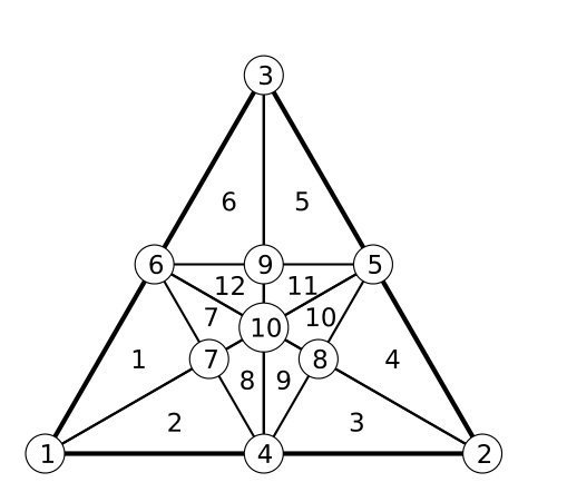 Figure 1
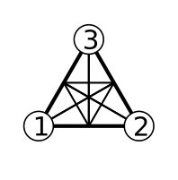 Figure 2
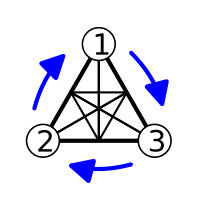 Figure 3
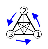 Figure 4
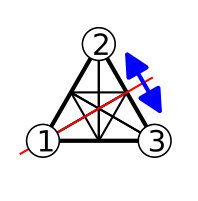 Figure 5
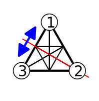 Figure 6
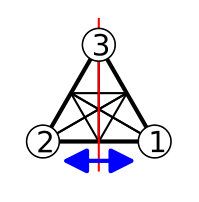 Figure 7
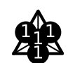 Figure 8
 Figure 9
 Figure 10
 Figure 11
 Figure 12
 Figure 13
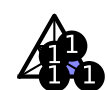 Figure 14
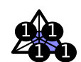 Figure 15
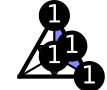 Figure 16
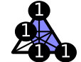 Figure 17
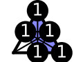 Figure 18
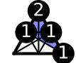 Figure 19
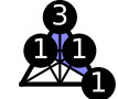 Figure 20
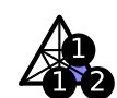 Figure 21
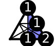 Figure 22
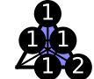 Figure 23
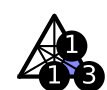 Figure 24
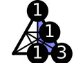 Figure 25
 Figure 26
 Figure 27
 Figure 28
 Figure 29
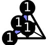 Figure 30
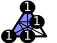 Figure 31
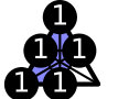 Figure 32
 Figure 33
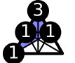 Figure 34
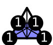 Figure 35
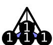 Figure 36
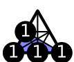 Figure 37
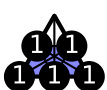 Figure 38
 Figure 39
 Figure 40