Testing a model for subphotospheric dissipation in GRBs: fits to Fermi data constrain the dissipation scenario
Bj\"orn Ahlgren, Josefin Larsson, Erik Ahlberg, Christoffer Lundman,, Felix Ryde, Asaf Pe'er

TL;DR
This study tests a photospheric dissipation model for GRB prompt emission using Fermi data, finding it explains some spectra but not all, and revealing correlations between luminosity and Lorentz factor.
Contribution
It provides the first direct fitting of a physically motivated photospheric model to Fermi GRB spectra, constraining dissipation radius and efficiency.
Findings
Approximately two thirds of spectra are not well-fit by the model.
The dissipation occurs at around 10^12 cm radius in successful fits.
A positive correlation between fireball luminosity and Lorentz factor is observed.
Abstract
It has been suggested that the prompt emission in gamma-ray bursts (GRBs) could be described by radiation from the photosphere in a hot fireball. Such models must be tested by directly fitting them to data. In this work we use data from the Fermi Gamma-ray Space Telescope and consider a specific photospheric model, in which kinetic energy of a low-magnetisation outflow is dissipated locally by internal shocks below the photosphere. We construct a table model with a physically motivated parameter space and fit it to time-resolved spectra of the 36 brightest Fermi GRBs with known redshift. We find that about two thirds of the examined spectra cannot be described by the model, as it typically under-predicts the observed flux. However, since the sample is strongly biased towards bright GRBs, we argue that this fraction will be significantly lowered when considering the full population. From…
Click any figure to enlarge with its caption.
 Figure 10
 Figure 11
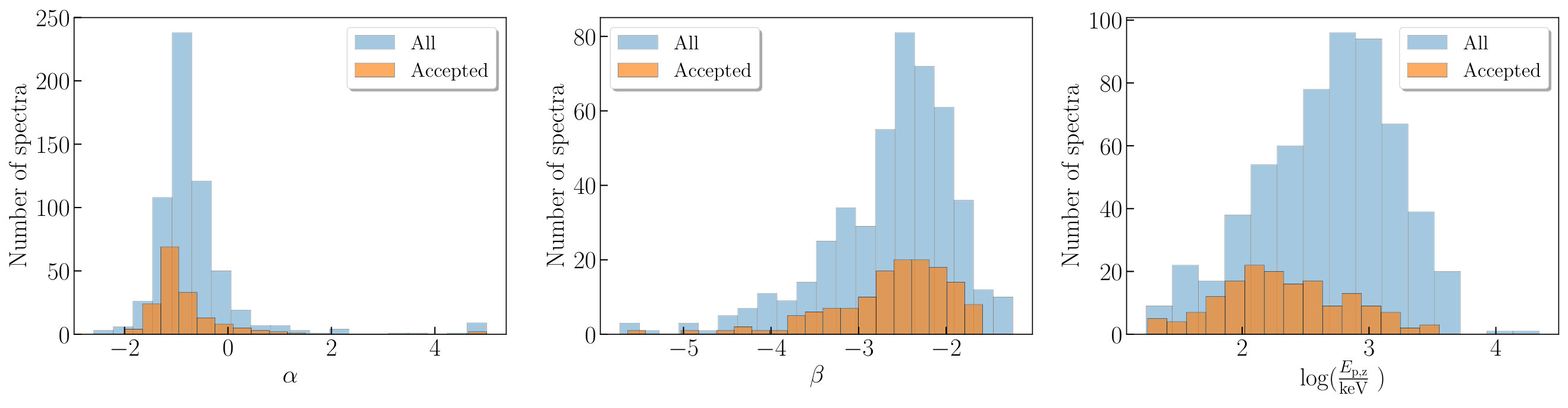 Figure 12
 Figure 13
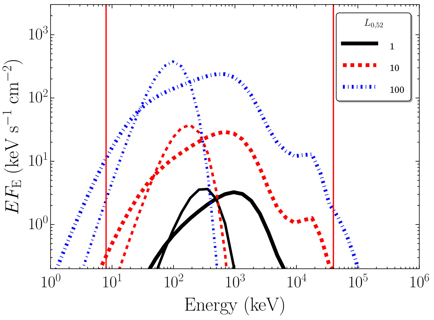 Figure 1
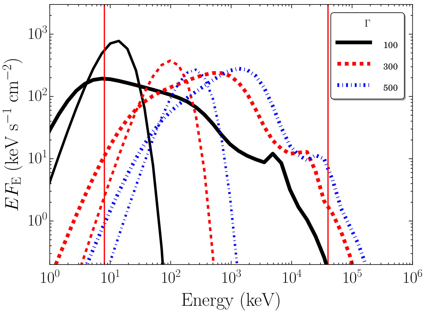 Figure 1
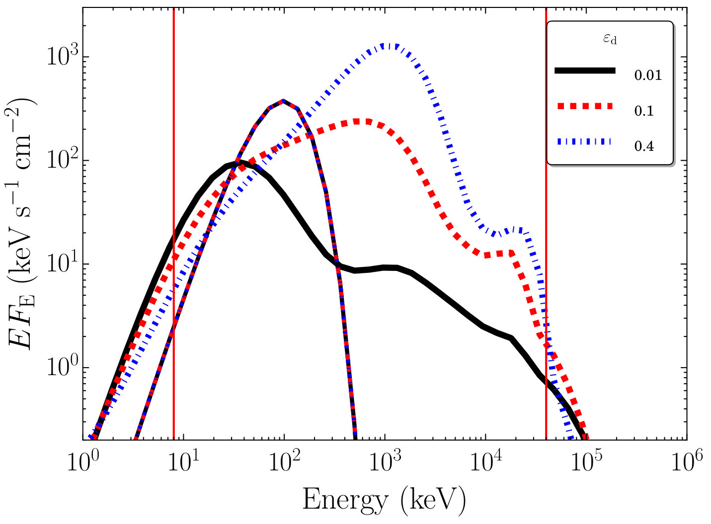 Figure 1
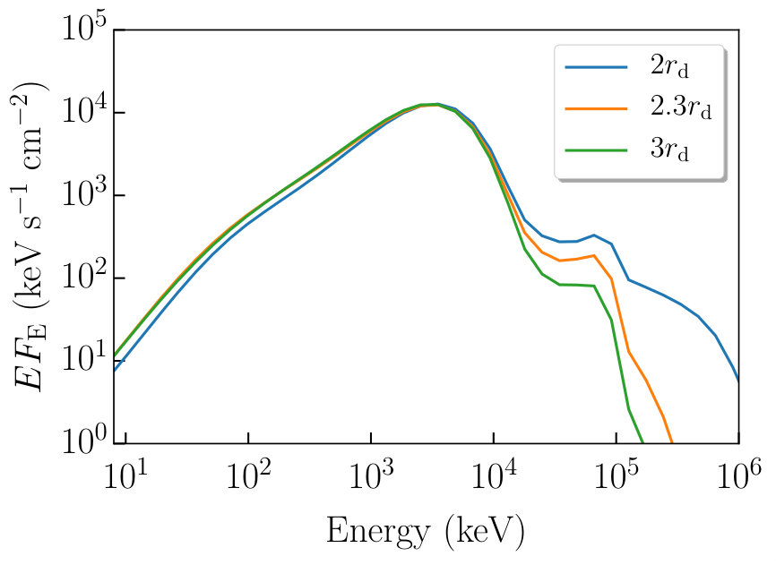 Figure 2
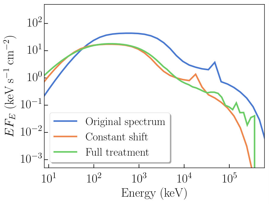 Figure 3
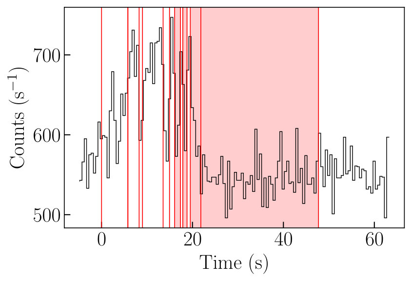 Figure 4
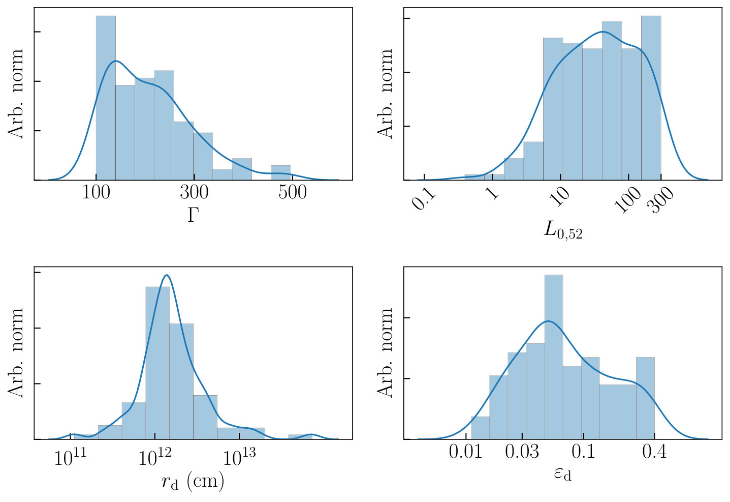 Figure 5
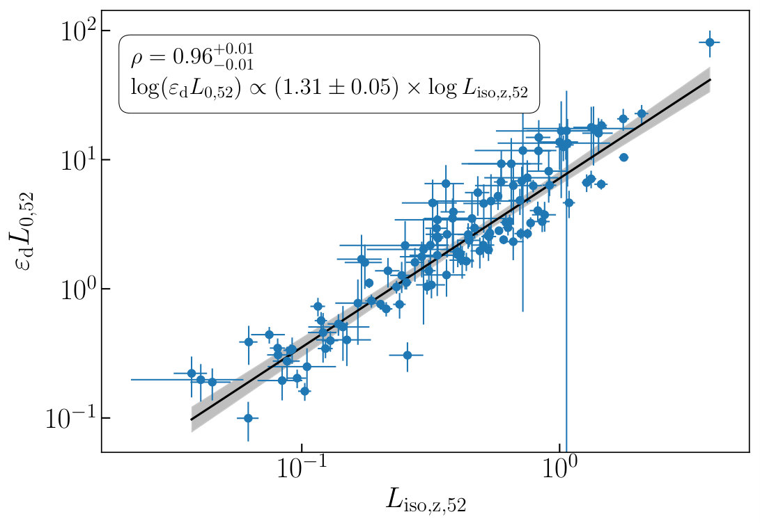 Figure 6
 Figure 6
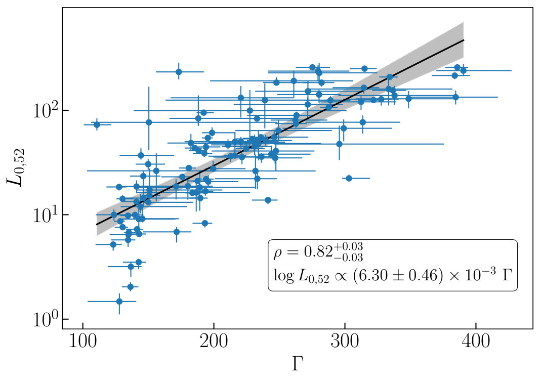 Figure 6
 Figure 7
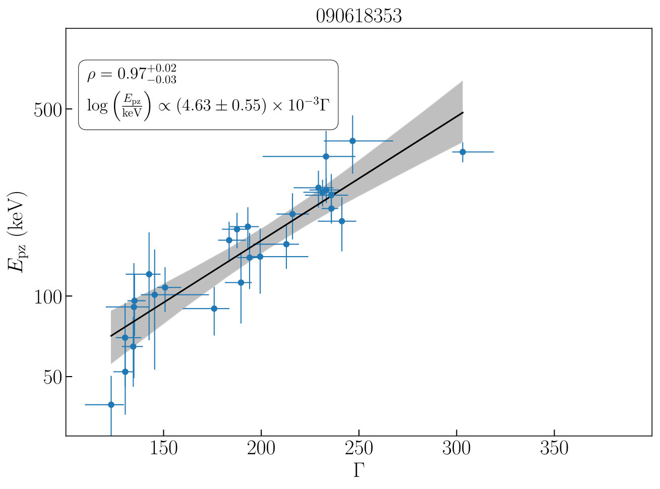 Figure 7
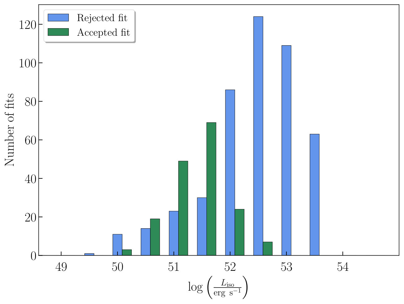 Figure 8
 Figure 9
 Figure 9
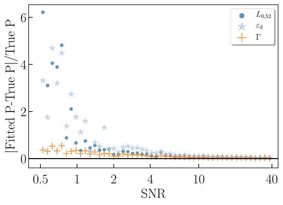 Figure 20
 Figure 21
 Figure 22
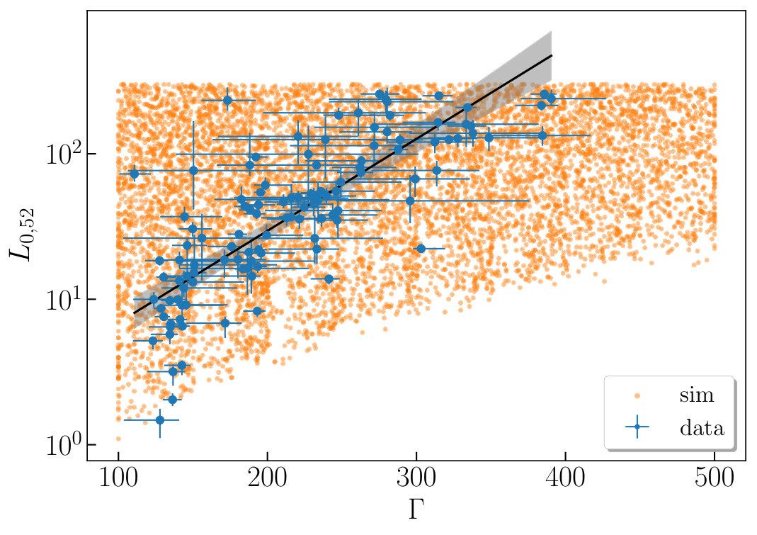 Figure 23
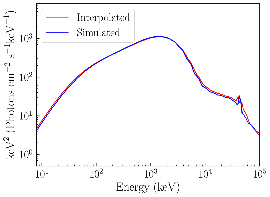 Figure 24
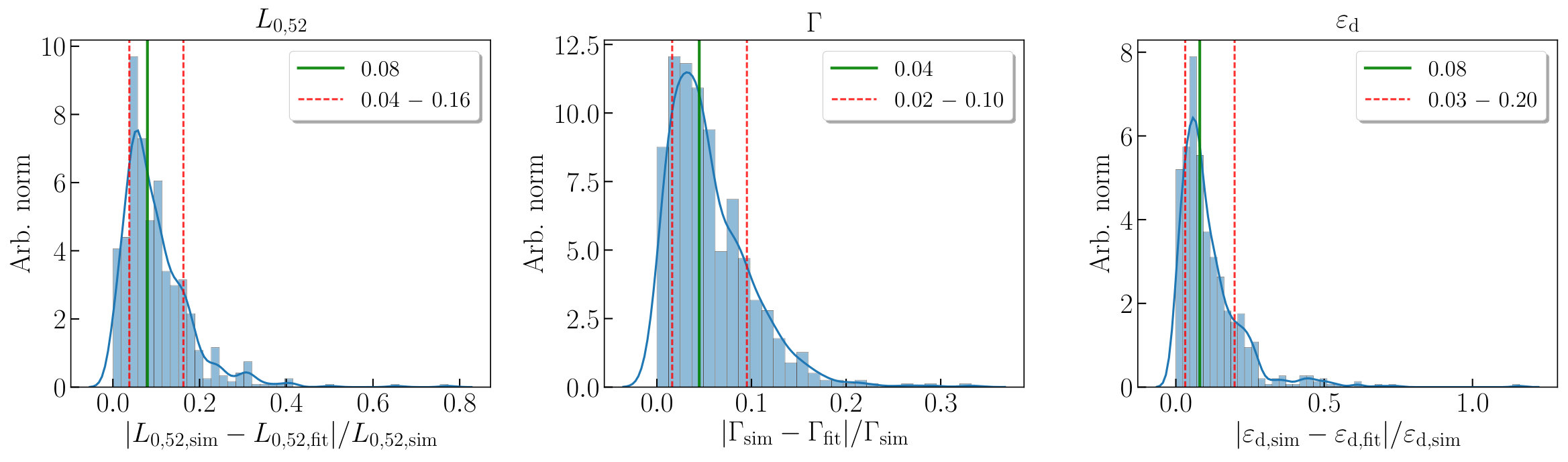 Figure 25
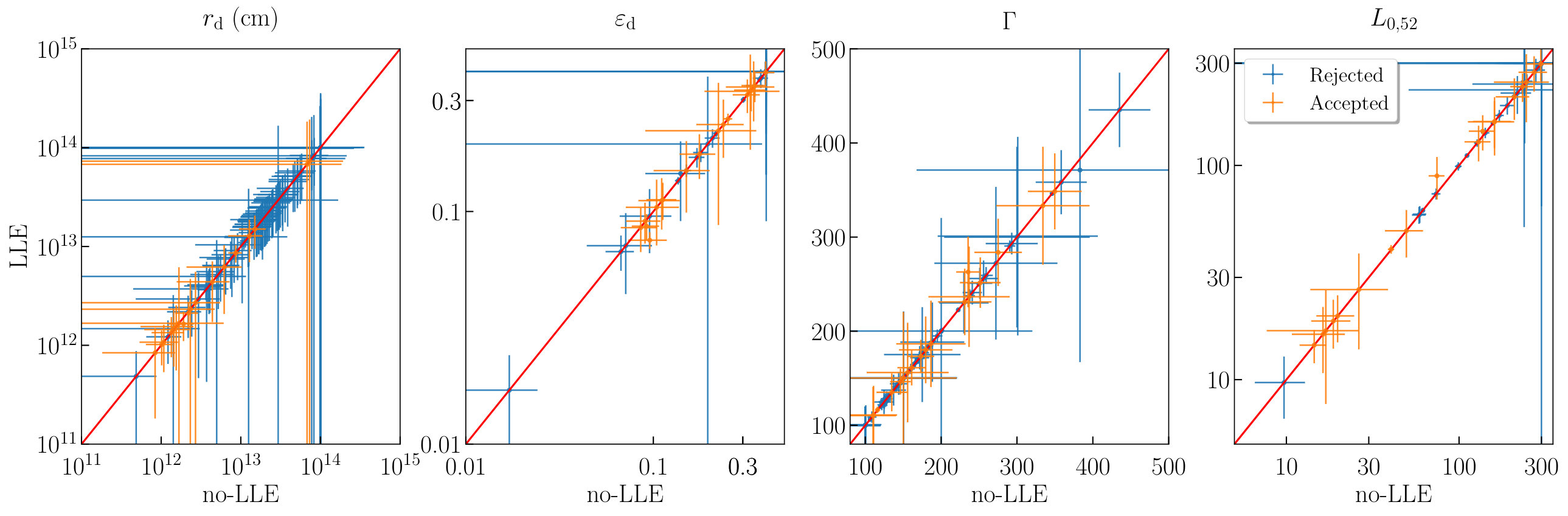 Figure 26
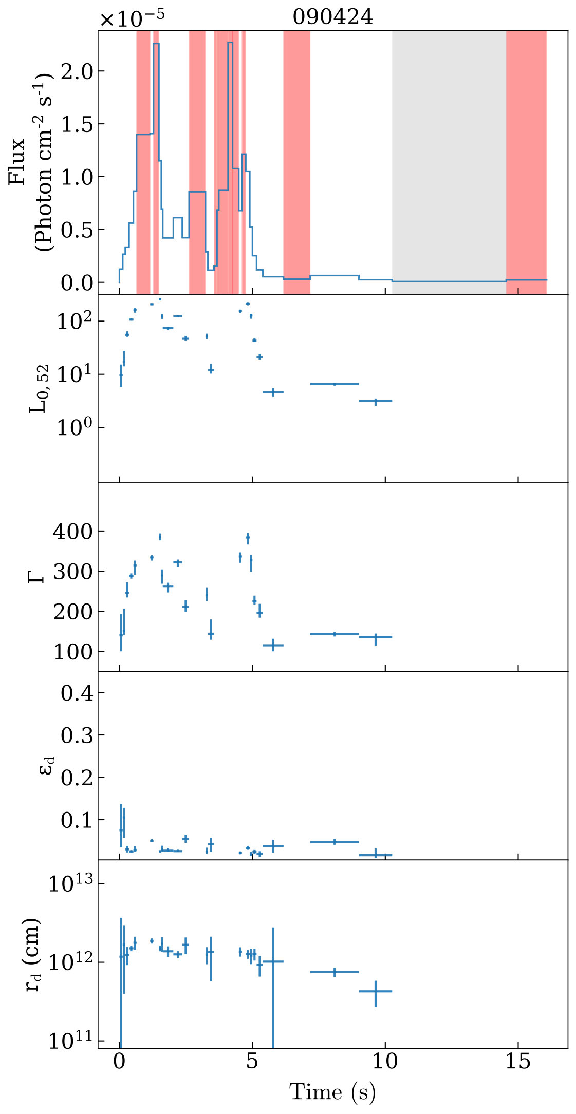 Figure 27
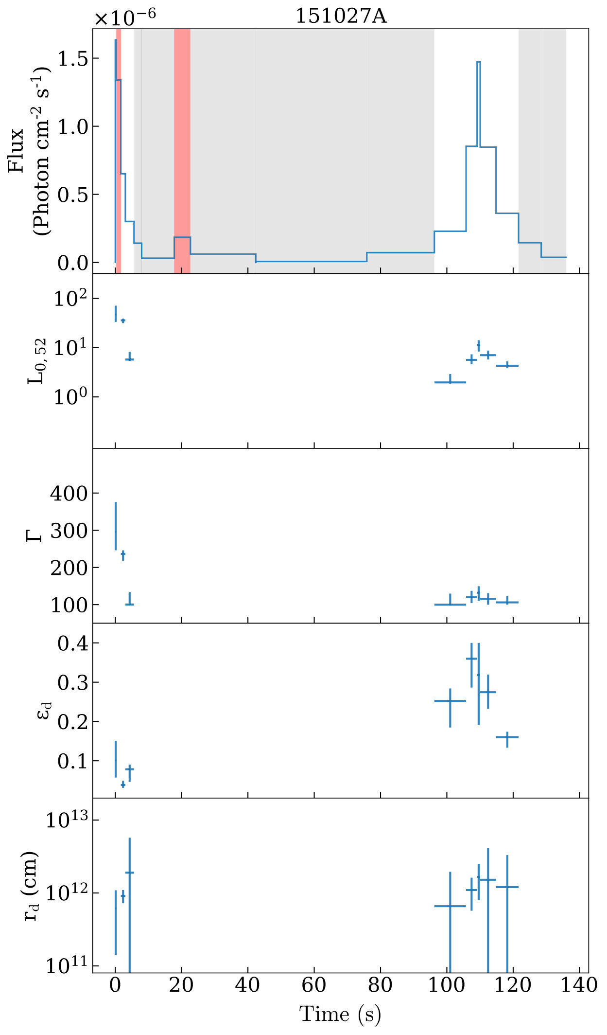 Figure 28
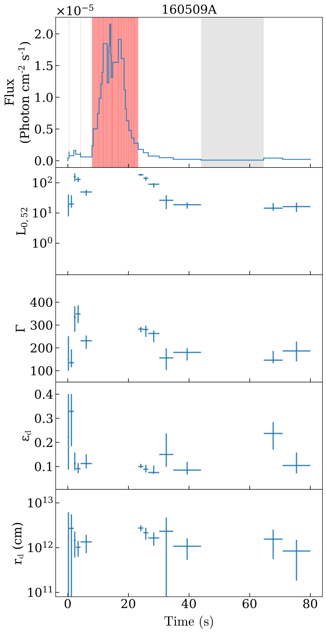 Figure 29
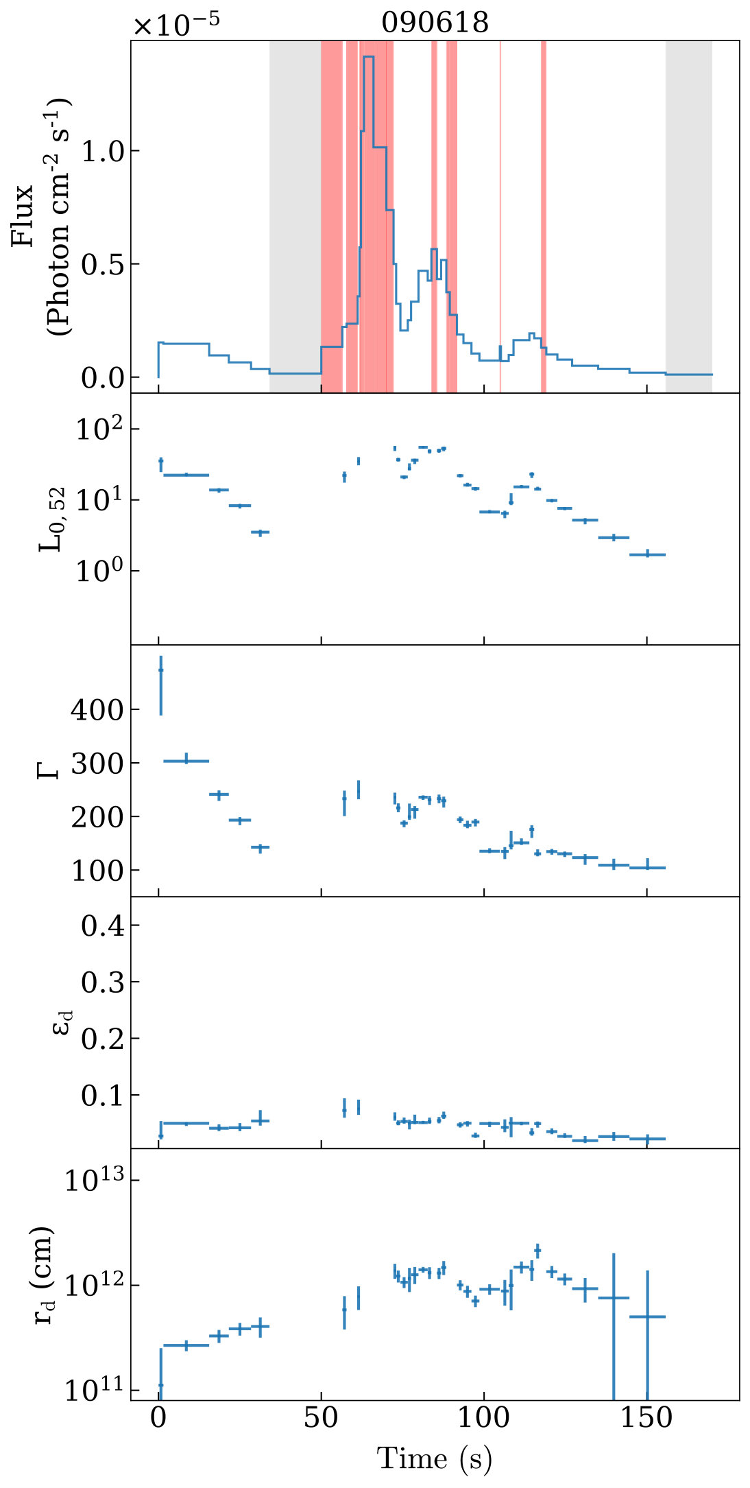 Figure 30
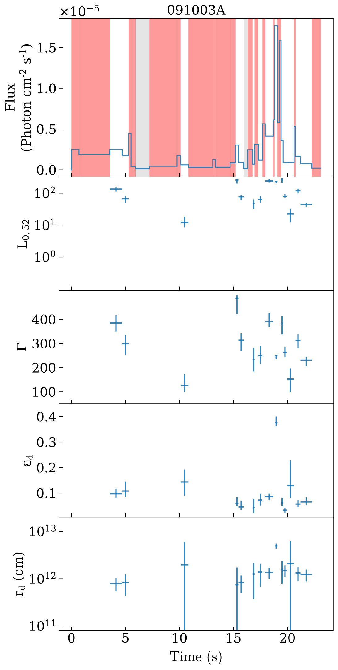 Figure 31
 Figure 32
 Figure 33
 Figure 34
 Figure 35
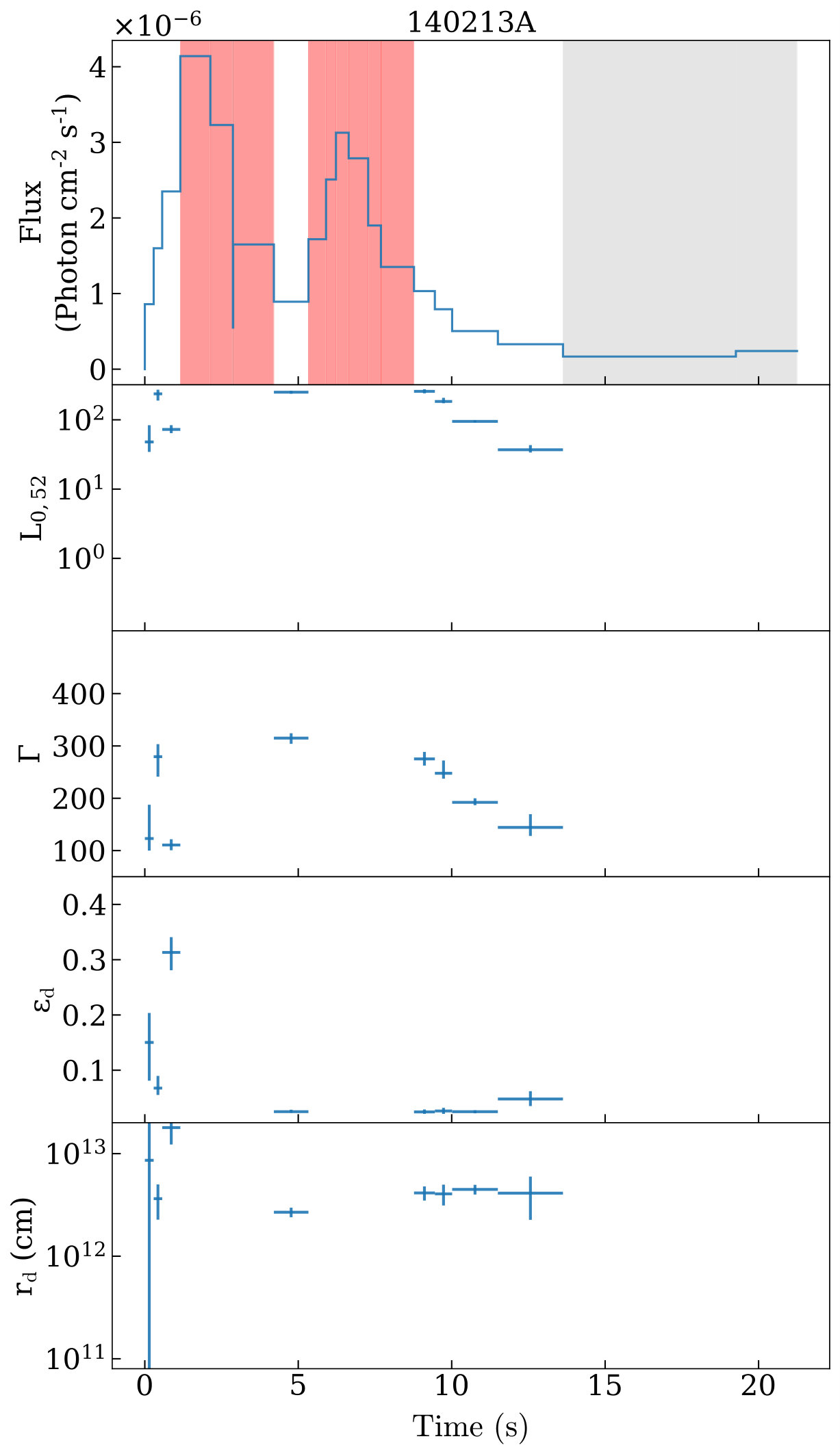 Figure 36
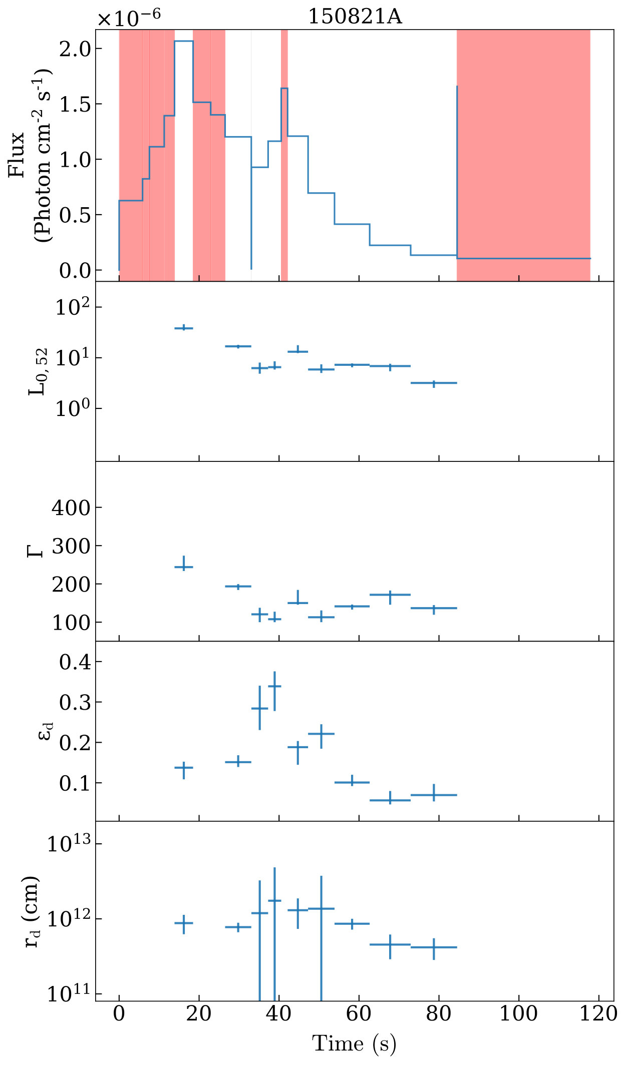 Figure 10
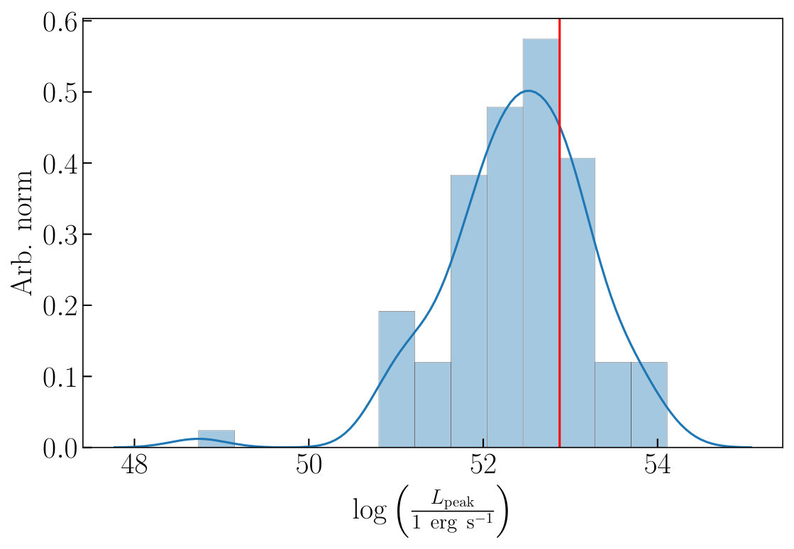 Figure 11
 Figure 12
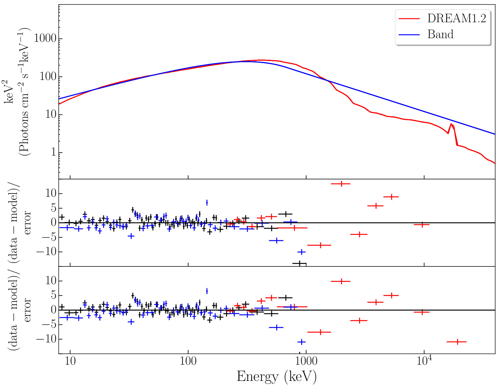 Figure 13
| GRB | T90 | Fluence | redshift |
| (s) | (erg cm-2) | ||
| 080916C | 63.0 | 6.03e-05 | 4.35 |
| 081121 | 42.0 | 1.53e-05 | 2.512 |
| 081221 | 29.7 | 3.00e-05 | 2.26 |
| 090323A | 135.2 | 1.18e-04 | 3.57 |
| 090424 | 14.1 | 4.63e-05 | 0.544 |
| 090516 | 123.1 | 1.72e-05 | 4.109 |
| 090618 | 112.4 | 2.68e-04 | 0.54 |
| 090902B | 19.3 | 2.22e-04 | 1.822 |
| 090926A | 13.8 | 1.47e-04 | 2.1062 |
| 090926B | 55.6 | 1.08e-05 | 1.24 |
| 091003A | 20.2 | 2.33e-05 | 0.8969 |
| 091127 | 8.7 | 2.07e-05 | 0.49 |
| 100414A | 26.5 | 8.85e-05 | 1.368 |
| 100728A | 165.4 | 1.28e-04 | 1.567 |
| 100814A | 150.5 | 1.49e-05 | 1.44 |
| 100906A | 110.6 | 2.33e-05 | 1.727 |
| 110731A | 7.5 | 2.29e-05 | 2.83 |
| 111228A | 99.8 | 1.81e-05 | 0.714 |
| 120119A | 55.3 | 3.87e-05 | 1.728 |
| 120711A | 44.0 | 1.94e-04 | 1.405 |
| 120716A | 237.1 | 1.44e-05 | 2.486 |
| 130215A | 143.7 | 1.86e-05 | 0.597 |
| 130420A | 105.0 | 1.16e-05 | 1.297 |
| 130518A | 48.6 | 9.46e-05 | 2.488 |
| 130925A | 215.6 | 8.48e-05 | 0.347 |
| 131105A | 112.6 | 2.38e-05 | 1.686 |
| 140206A | 27.3 | 1.55e-05 | 2.73 |
| 140213A | 18.6 | 2.12e-05 | 1.2076 |
| 140423A | 95.2 | 1.81e-05 | 3.26 |
| 140512A | 148.0 | 2.93e-05 | 0.725 |
| 141028A | 31.5 | 3.48e-05 | 2.33 |
| 150314A | 10.7 | 8.16e-05 | 1.758 |
| 150403A | 22.3 | 5.47e-05 | 2.06 |
| 150821A | 103.4 | 5.21e-05 | 0.755 |
| 151027A | 123.4 | 1.41e-05 | 0.81 |
| 160509A | 369.7 | 1.79e-04 | 1.17 |
| Burst | Time bin | ||||
| ( cm) | |||||
| 090424 | 0.0-0.1 | ||||
| 090424 | 0.1-0.2 | ||||
| 090424 | 0.2-0.4 | ||||
| 090424 | 0.4-0.5 | ||||
| 090424 | 0.5-0.6 |
| burst | Analysed | |
| Accepted | ||
| spectra | ||
| 080916C | 15 | 0 |
| 081121 | 9 | 0 |
| 081221 | 18 | 0 |
| 090323A | 23 | 0 |
| 090424 | 32 | 21 |
| 090516 | 0 | 0 |
| 090618 | 42 | 30 |
| 090902B | 61 | 1 |
| 090926A | 28 | 1 |
| 090926B | 4 | 0 |
| 091003A | 32 | 14 |
| 091127 | 23 | 18 |
| 100414A | 21 | 2 |
| 100728A | 13 | 1 |
| 100814A | 4 | 1 |
| 100906A | 14 | 3 |
| 110731A | 12 | 0 |
| 111228A | 17 | 10 |
| 120119A | 14 | 2 |
| 120711A | 34 | 6 |
| 120716A | 6 | 0 |
| 130215A | 3 | 2 |
| 130420A | 2 | 1 |
| 130518A | 23 | 2 |
| 130925A | 20 | 2 |
| 131105A | 17 | 11 |
| 140206A | 11 | 0 |
| 140213A | 17 | 8 |
| 140423A | 0 | 0 |
| 140512A | 7 | 4 |
| 141028A | 13 | 1 |
| 150314A | 16 | 0 |
| 150403A | 20 | 1 |
| 150821A | 18 | 9 |
| 151027A | 10 | 8 |
| 160509A | 35 | 12 |
| total | 634 | 171 |
Peer Reviews
No public reviews on file for this paper yet. If you reviewed it on a platform where reviews are public (OpenReview, ICLR, NeurIPS, ICML), you can paste yours below so the community can read it here.
Videos
No videos yet. Explain this paper in a talk, walkthrough, or lecture? Add one.
Testing a model for subphotospheric dissipation in GRBs: fits to Fermi data constrain the dissipation scenario
Björn Ahlgren1, Josefin Larsson1, Erik Ahlberg1, Christoffer Lundman1, Felix Ryde1, Asaf Pe’er2,3
1KTH Royal Institute of Technology, Department of Physics, and the Oscar Klein Centre, AlbaNova, SE-106 91 Stockholm, Sweden
2Physics Department, University College Cork, Cork, Ireland 3Department of Physics, Bar-Ilan University, Ramat-Gan 52900, Israel E-mail: [email protected]
(Accepted 2019 January 09. Received 2019 January 09; in original form 2018 January 24)
Abstract
It has been suggested that the prompt emission in gamma-ray bursts (GRBs) could be described by radiation from the photosphere in a hot fireball. Such models must be tested by directly fitting them to data. In this work we use data from the Fermi Gamma-ray Space Telescope and consider a specific photospheric model, in which kinetic energy of a low-magnetisation outflow is dissipated locally by internal shocks below the photosphere. We construct a table model with a physically motivated parameter space and fit it to time-resolved spectra of the 36 brightest Fermi GRBs with known redshift. We find that about two thirds of the examined spectra cannot be described by the model, as it typically under-predicts the observed flux. However, since the sample is strongly biased towards bright GRBs, we argue that this fraction will be significantly lowered when considering the full population. From the successful fits we find that the model can reproduce the full range of spectral slopes present in the sample. For these cases we also find that the dissipation consistently occurs at a radius of cm and that only a few percent efficiency is required. Furthermore, we find a positive correlation between the fireball luminosity and the Lorentz factor. Such a correlation has been previously reported by independent methods. We conclude that if GRB spectra are due to photospheric emission, the dissipation cannot only be the specific scenario we consider here.
keywords:
gamma-ray burst: general – radiation mechanisms: thermal – gamma-ray burst:
††pubyear: 2019††pagerange: Testing a model for subphotospheric dissipation in GRBs: fits to Fermi data constrain the dissipation scenario–E
1 Introduction
Prompt GRB emission mechanisms are still a matter of debate, and remain an unsolved problem in GRB physics. The principal approach to finding the origin of GRB prompt emission has been to fit spectra with empirical functions and use the best-fitting parameters to constrain different emission scenarios. For a considerable time the empirical Band function (Band et al., 1993), a smoothly broken power law, has been the predominant way of fitting these spectra. The Band function often provides good fits to the prompt emission spectra and the fits have commonly been interpreted in terms of synchrotron emission (Tavani, 1996; Briggs et al., 1999; Abdo et al., 2009; Zhang et al., 2016). However, it has been shown that synchrotron radiation cannot consistently produce the full distribution of spectral shapes we observe when fitting with the Band function, including the low-energy slope (Preece et al., 1998) and the spectral width of the peak (Axelsson & Borgonovo, 2015; Yu et al., 2015). In addition, the Band function does not represent a physical scenario, and in order to obtain physical information we must instead ultimately use a physically motivated model and fit to data (see also Burgess et al. 2014a, 2015).
Observations of GRBs with spectra close to blackbodies (BBs) (Ryde, 2004; Ghirlanda et al., 2013; Larsson et al., 2015), as well as spectra described by a BB and an additional component (Ryde et al., 2010; Guiriec et al., 2011; Axelsson et al., 2012; Burgess et al., 2014b; Arimoto et al., 2016), suggest that at least some bursts have prompt emission of a photospheric origin. Conversely, for most GRBs, the simplest models of photospheric emission cannot provide an adequate description of the observed spectra. In particular, the low-energy spectral slope of most bursts is significantly softer than a Planck function.
It has been shown that more realistic photospheric models will result in spectra that are broader than a Planck function. The broadening can be a result of, e.g., subphotospheric dissipation (Rees & Mészáros, 2005; Pe’er et al., 2006; Giannios, 2006; Beloborodov, 2010; Vurm et al., 2011; Chhotray & Lazzati, 2015), or geometric effects (Pe’er, 2008; Lundman et al., 2013). Subphotospheric dissipation has previously been invoked to interpret the ‘top-hat’ spectral shape of GRB 110920 (Iyyani et al., 2015) and the broadening of the initially very narrow spectrum of GRB 090902B (Ryde et al., 2011). Though subphotospheric dissipation has been used to describe several bursts, the different model scenarios must be examined further, particularly using larger data samples and proper techniques when fitting models to data.
In our previous work (Ahlgren et al., 2015), A15 from here on, we fitted a model for subphotospheric dissipation to prompt GRB emission data from the Fermi Gamma-ray Space Telescope. This was the first time such a model was fitted to data and the study served as an important proof-of-concept. Specifically, we fitted GRB 090618, which can also be described by a Band function with typical parameters, and GRB 100724B, which has previously been fitted with a composite Band+BB model. The results showed that subphotospheric dissipation is a viable description of both bursts and justified further investigations.
In this work we build on the work presented in A15 by increasing the model parameter space and by including approximate adiabatic cooling. We have also significantly expanded our sample, now analysing 36 bursts, and have performed Monte Carlo simulations to quantify some of the model’s inherent uncertainties. We also consider parameter correlations and physical implications.
The main goal of the work is to test the scenario of localised dissipation by internal shocks below the photosphere in a low-magnetisation outflow. We emphasise that the constraints found in the paper do not apply to photospheric emission in general or other dissipation scenarios. We confine our study to the case where almost all the dissipated energy goes into the electrons and explore the effects of three free parameters, as described in section 2.2. The second main objective is to present the continued development of our table model, which we plan to make publicly available.
The paper is organised as follows: section 2 describes the physical scenario and the table model implementation. In section 3 we describe our data sample, binning and fitting procedure. Section 4 presents the results and section 5 is the discussion. Section 6 is summary and conclusions. Finally, in appendices A-E we present more technical details about the model and analysis.
2 The Model
2.1 Physical scenario
In this paper we consider the same physical model as in A15. It is a model based on the fireball model, specifically a hot fireball, using a kinetic code by Pe’er & Waxman (2005). We described this model in A15, but for completeness we present an overview here as well. Any deviations from the model as stated in A15 will be explicitly pointed out. Note that all quantities in this section are in the observer frame unless otherwise stated.
In the fireball model (see e.g. Pe’er 2015 for a recent review), an isotropic equivalent luminosity, erg s*-1*, is emitted from the central engine in the form of baryons, electrons, -fields, and photons. The outflow starts at the initial jet radius, , where the bulk Lorentz factor is . The photons give rise to a radiative pressure which accelerates the outflow into highly relativistic collimated jets. The outflow is accelerated until the saturation radius, . At this point the outflow is in thermal equilibrium and coasts with constant . The baryons, mainly protons, carry the bulk of the kinetic energy of the outflow. In our model we define the dissipation radius as , where is the optical depth due to the baryonic electrons (i.e. the electrons which are associated with the protons of the outflow). At this radius we dissipate a fraction of the kinetic energy of the protons, out of which the fraction goes to electrons and a fraction is used to generate magnetic fields.
The dissipation creates a non-equilibrium situation between the photon bath and the heated electron population, where they interact through Compton and inverse Compton scattering, as well as pair production and pair annihilation. We also treat synchrotron radiation and synchrotron self-absorption. It is assumed that electrons are injected as a Maxwellian distribution with a dimensionless temperature, , in the range of 5.5 - 220. Both newly injected electrons and the existing population will interact with the photons. Before the dissipation essentially all energy is carried by the baryons in the jet. After the dissipation the dissipated energy has been transferred to the photons, but the baryons still carry the majority of the energy.
Possible dissipation mechanisms in GRB jets include magnetic reconnection (Thompson, 1994; Drenkhahn & Spruit, 2002; Giannios & Spruit, 2005; Lyutikov, 2006), hadronic collisions (Beloborodov, 2010) or internal shocks (Kobayashi et al., 1997; Daigne & Mochkovitch, 1998; Rees & Mészáros, 2005). In our current implementation we are working with the internal shocks paradigm by assuming that . We also assume that the dissipation is a continuous process localised between and . Note that this is different from the scenario with continuous subphotospheric dissipation throughout the jet employed in e.g. Vurm & Beloborodov (2016).
A caveat is that large a value of would remove the majority of the kinetic energy of the outflow and would inevitably decelerate it. This in turn may lead to a re-acceleration phase, which is not treated in our code. We therefore avoid the corresponding part of the parameter space. Since the energy is passed to either the electrons or the magnetic fields, this translates to being the constrained quantity. We have decided to require to minimise this effect while still keeping a large amount of parameter space to work with. Even at this level of dissipation one could expect a second acceleration phase (Bégué & Iyyani, 2014), but we expect this to have a limited impact on our results.
There are additional physical effects not accounted for in the code. Examples include spatial effects, such as the aforementioned geometric broadening, the jet opening angle, jet hydrodynamics (e.g. Lazzati et al. 2009) and the effects from a fuzzy photosphere (Beloborodov, 2011; Bégué et al., 2013). Finally, we do not at this stage consider neutrino emission or afterglow predictions.
2.2 Table model
The XSPEC table model implementation (Arnaud et al., 1999) allows us to build a numerical model from simulated spectra. A table model consists of a grid of model spectra, corresponding to different parameter values. Interpolation between spectra is used to obtain spectral shapes between the grid points. Using our numerical code we perform a large number of simulations for different parameter values, spanning the grid
[TABLE]
which yields a total of 891 grid points. Note that other physical parameters often discussed in the context of subphotospheric dissipation, such as and , are derived quantities according to the expressions defined in section 2.1. Furthermore, the model obtains a normalisation and redshift as two additional parameters when it is implemented in XSPEC. These two parameters are kept constant during the fits, with the redshift given from observations and the normalisation set by the luminosity distance.
As in A15 we let and , in order to test the scenario where almost all the energy goes into electrons and where we have no significant contribution from synchrotron. We note that this leaves . However, this simply means that the remaining energy is never dissipated. The main difference to the parameter space employed in A15 is that we now have set instead of letting it be a free parameter. This represents a scenario with the dissipation occurring moderately deep in the outflow. There are several reasons for this choice. Firstly, testing shows that most fits prefer high values of , with very few spectra being described by a few. However, at this parameter turns out to be relatively insensitive. Changes in at these values usually result in small changes of the fit statistic, predicted spectral shape in the part of the GBM energy range where the statistics are best, and small changes in other model parameters. Additionally, cannot always be given a meaningful physical interpretation. Due to significant pair production, it does not directly correspond to the number of scatterings in the outflow, it also does not correspond directly to . Finally, keeping fixed decreases degeneracies in the model. Compared to the model in A15, we have also expanded to lower values, from 0.1 down to 0.01, and made all parameters more tightly spaced in the grid. These improvements from the previous model reduce uncertainties pertaining to interpolation in the grid (see discussion in appendix B).
With these modifications we have captured most of the physically relevant parameter space for the three free parameters of our model. The main exception is , which could in principle lie outside the range 100-500, although most Lorentz factors are expected to lie within our parameter range, see e.g. Ghirlanda et al. (2018). The upper bound for is set by dynamical concerns, as discussed in section 2.1, and the lower bound by efficiency requirements. To a good approximation, the fireball luminosity, , relates to the observed isotropic equivalent luminosity as . Hence, the maximum fireball luminosity is , for a maximal observed luminosity, . Atteia et al. (2017) find the limit erg for observed isotropic energies. Assuming a typical duration for long GRBs of s, (Bhat et al., 2016b), we obtain the limits and , for the minimum and a more typical , respectively. Thus, considering variations in and burst duration, the limit, , we have set is reasonable, though not absolute. In section 5.2 we discuss the implications of our choices of parameter limits.
In A15 we referred to our table model as DREAM (Dissipation with Radiative Emission as A table Model). Since the goal is to make DREAM publicly available, we adopt a naming convention to help discriminate between and refer to the different versions of the table model as we develop it. The first number relates to the physical scenario considered when generating the model spectra, using the numerical code from Pe’er & Waxman (2005). The physical scenario decides the parametrisation in the numerical code, without changing the underlying numerical scheme or the relevant physics. The second number denotes which grid has been used, including minor revisions such as post-processed treatment of adiabatic cooling. With this naming convention, the model of A15 becomes DREAM1.1, and the model herein is DREAM1.2. Throughout the paper, "model" is, unless otherwise stated, referring to the table model, DREAM1.2. "Physical scenario" is used to refer to the underlying physical model (subphotospheric dissipation by internal shocks with negligible magnetic fields). Any references to a "code" refers to the numerical code presented in Pe’er & Waxman (2005).
In Fig. 1 we exemplify some spectral shapes as functions of the free parameters. As the dependency of spectral shape on our parameters is non-linear and we have a multi-dimensional parameter space, it is not possible to give an exact accounting for how the spectral shape changes with any single parameter. However, there are some clear features that are typical to certain parameters. Using Fig. 1 we give a qualitative overview of the main impact of our parameters on the spectral shapes.
Generally, the spectrum will consist of a BB peak and an inverse Compton peak at higher energies. For a small amount of dissipation we expect the BB peak to dominate and to yield a single-peaked spectrum. When the dissipation increases the inverse Compton peak becomes more pronounced and we can obtain a single-peaked spectrum with the peak at high energies or, if the peaks are comparable in strength, we obtain a flat, ‘top-hat’ shape, or a double peaked spectrum. For low values of , as we consider here, the spectrum is dominated by inverse Compton scattering and the contributions from synchrotron radiation are negligible. Another feature is the pair production peak at .
The parameter with the clearest effect on the spectra is the fireball luminosity, , which mainly sets the flux, since it is positively correlated to the number of photons in the spectrum and spans several orders of magnitude. Additionally, has the effect of setting the distance between the peaks in the spectrum caused by inverse Compton scattering. This is caused by the electron temperature being independent of , while the temperature of the seed BB is inversely dependent on (Pe’er & Waxman, 2005).
One of the major effects of is the Doppler shift, which sets the observed energies of the spectrum. Additionally, the initial BB temperature increases as a function of , which sets the position and normalisation of the first peak in the spectrum. Increasing also yields a higher pair multiplicity, which is why we see the spectra with increasing in Fig. 1 get increasingly thermalised as increases. Note that this is different from the commonly assumed solution to the compactness problem, where an increasing suppresses photon-photon annihilation. Due to the assumption that , will alter quantities such as volume and electron number, resulting in a net effect of positive correlation between and pair multiplicity. Note that also contributes to setting the number of photons, but with an inverse dependence. However, due to its limited range and its other effects on the spectrum, it is the luminosity which works as the main driver of the predicted flux.
The last free parameter of our model, , mainly changes the comoving electron temperature, , (Pe’er et al., 2006). This sets the normalisation of the inverse Compton peak, with a higher resulting in a stronger peak. However, the position of the this peak is not sensitive to for much of the parameter space. This is because the first up-scattered photons may pair produce and yield a population of cooler electrons, usually outnumbering the baryonic electrons by a factor of several. The observed inverse Compton peak in the spectrum is a result of multiple scatterings with electrons of a wide energy distribution, making its position almost independent of the initial electron temperature.
2.3 Additional scatterings and adiabatic cooling
In A15 the numerical code was run only as long as there was dissipation, i.e. between and . This takes care of the most important physics and relevant processes, but it does not include the last of the scatterings, between and . Running the code all the way to the photosphere from an optical depth of is not feasible with the current set-up. However, it is sufficient to run the code a fraction of the way to the photosphere to capture most of the spectral changes occurring after the dissipation. In Fig. 2 we show examples of spectral shapes as a function of where the simulation ends. It is clear from the figure that there is little change already after In this work we have chosen to let the code run between and . We note that the factor of 2.3 was found empirically to be a good trade-off between computational efficiency and capturing changes in the spectral shape.
As stated in A15, the code does not in its current form include adiabatic cooling. However, we would expect adiabatic cooling to yield a shift of the entire spectrum to lower energies., see e.g. Pe’er & Waxman (2004). This effect is caused by a continuous cooling of the photons as they do work on the outflow for as long as they scatter, i.e. roughly as long as in our scenario. In a more realistic scenario we would also expect the photons to start decoupling before , mainly leading to a broadening of the spectral shape (Beloborodov, 2011; Bégué et al., 2013). The photons continuously isotropise during collisions by converting internal photon energy to bulk kinetic energy of the outflow, and thus stay isotropic in the rest frame. As long as we have a thermal spectrum this results in a constant shift of the spectrum to lower energies. For non-thermal spectra, each scattering will also distort the spectral shape. We begin by considering only pure adiabatic cooling. As it is a constant shift of the spectrum, this effect may be treated by analytic post-processing. We introduce an adiabatic cooling factor , where is the optical depth at the end of the dissipation, with which we simply shift the spectrum. Hence the number of photons at a given energy, is shifted such that , with and where is the shifted energy. For more details on the adiabatic cooling factor, including its limitations, see Beloborodov (2011) and Bégué et al. (2013). The constant shift using is an approximation to taking into account all scatterings up to the photosphere.
In Fig. 3 we show an example of an original model spectrum, as calculated from our numerical code, compared with the spectrum after having applied the adiabatic cooling factor, as well as the spectrum after a full treatment of all scatterings, adiabatic cooling and geometric effects up to the photosphere. The full treatment was performed using a numerical code from Lundman et al. (2017), which dynamically couples hydrodynamics to Monte Carlo radiative transfer inside a spherical outflow. The radiation can then be followed as it cools adiabatically, and self-consistently decouples from the flow at a fuzzy photosphere. This code can be used to study the spectral evolution after dissipation. However, the code is computationally very expensive, which prevents us from using it for all spectra. Fig. 3 illustrates that our approximation of a constant shift yields good agreement of the integrated model flux. However, we note a small discrepancy between the spectrum with the constant shift approximation and the full treatment in the low energy slope keV. This effect is a result of the full treatment taking a fuzzy photosphere and geometric effects into account. We thus conclude that the approximate treatment of the adiabatic cooling is good, and that it represents a significant improvement over the original model spectrum, but that the inclusion of geometric effects would lead to a slightly softer low-energy slope.
3 Fitting with the model
3.1 Data sample
Our sample contains the brightest GRBs with known redshifts observed by Fermi before 2016-06-01. The known redshift111From http://www.mpe.mpg.de/~jcg/grbgen.html. helps us fix the normalisation parameter of the model spectrum via the corresponding luminosity distance, instead of leaving it as a free parameter. This is important because we want to be able to test the model’s ability to correctly predict the GRB flux. We chose a fluence cut of erg cm-2, in order to allow us to perform a time-resolved analysis with good signal strength. The resulting sample contains 36 GRBs, listed in Table 1.
For all GRBs we use Time Tagged Event (TTE) data from the Gamma-ray Burst Monitor (GBM) NaI and BGO detectors (Meegan et al., 2009). We select detectors by the scheme outlined in Bhat et al. (2016a), choosing up to three NaI detectors with an angle towards the source lower than 60\hbox{{}^{\circ}} as well as the BGO detector with the lowest angle towards the source. The energy range fitted was 8–1000 keV (NaI) and 200 keV – 40 MeV (BGO).
There are also LAT-LLE data available at high energies for nine bursts in the sample (GRB 080916C, GRB 090323A, GRB 090902B, GRB 090926A, GRB 110731A, GRB 130518A, GRB 141028A, GRB 150403A and GRB 160509A). The LLE data are a type of LAT data designed for the use with bright transients to bridge the energy range of the LAT and GBM (Pelassa et al., 2010). The LLE data (pass7) were obtained using gtburst version v02-01-03p50 and *Fermi *Science Tools version v9r32p5. The fitted energy range is 30–100 MeV. As noted in section 2.3, it is in this energy range our model has the largest uncertainties. However, we note that the inclusion or exclusion of the LLE data has little to no effect on the results (see appendix C for a discussion on the impact of the LLE data on our analysis).
3.2 Time-resolved spectral analysis
Our spectral analysis is time-resolved, using Bayesian blocks (Scargle et al., 2013) as binning method222We use the python implementation v1.1.1.1 of the algorithm from the Fermi Science Tools. The algorithm is performed on unbinned TTE data, with the false alarm rate parameter . We perform the binning using the NaI detector with the lowest angle of incidence. All signal-to-noise ratio (SNR) presented are also calculated from this detector. The background is fitted with polynomials. We account for repointing of the spacecraft and temporal evolution in the background by using rsp2 responses when available.
Bayesian blocks with an SNR cut is the most appropriate choice of binning given our model. The model does not include any time-evolution of the physical properties of the jet, meaning that any spectral evolution observed is assumed to be caused by central engine activity. Hence we assume constant central engine activity and no spectral evolution in each time bin we analyse. A constant central engine activity may be expected to give rise to a constant Poisson rate of photons in the light curve, which is what we recover with the Bayesian blocks scheme. However, this method may yield bins with a very low SNR. Thus, an SNR cut of was placed on the bins in accordance with what we found in the validation tests (see appendix A). We use an expression for the SNR as derived in Vianello (2018), for a Poisson measurement and a Gaussian background. Previous work by e.g. Yu et al. (2016) also employs an SNR requirement when performing time-resolved spectral analysis. The large difference in the level of the SNR cut between our work and theirs is a result of the different expressions used for calculating the SNR. See also Burgess (2014) for a discussion about different binning techniques, and Worpel & Schwope (2015) for general transient timing using Bayesian blocks.
In Fig. 4 we show an example of a light curve binned with Bayesian blocks, including 4 bins excluded at SNR. Our burst sample, defined in section 3.1, contains two bursts which yield no bins above the SNR threshold and are thus not analysed. The bursts which did not make the SNR cut are GRB 090516 and GRB 140423A. In total 145/779 bins are removed before analysis due to low SNR, giving us 634 time bins to analyse.
The analysis is performed using PyXspec, a python implementation of HEASARC’s XSPEC 12.8.1g, with pgstat statistics and with PHA (Pulse Height Analyser) data. We fit both our table model, DREAM1.2, as well the Band function, since the latter is used as a standard function in the field. We want to examine possible correlations between Band function parameters (i.e. the low energy slope, , the peak energy, , and the high energy slope, ), and the model parameters of DREAM1.2.
We note that the finite resolution of the table model grid results in additional uncertainties to those found from the regular fitting with Maximum Likelihood. Examining the points in the parameter space where we expect the largest resolution-related uncertainties, we find the median of the uncertainties to be less than per cent, depending on the parameter. and have the largest uncertainties. This evaluation is presented in appendix B. These uncertainties are not propagated into further analyses.
We have tested for effective area corrections between the detectors and find that the results do not change significantly if we allow for this correction or not. The size of the errors on fitted parameters are also not systematically or significantly affected. We present the fit results obtained without effective area corrections.
We assume standard -CDM cosmology with a Hubble constant of , a cosmological constant, and a matter density , (Planck Collaboration et al., 2014). All uncertainties are 1 unless otherwise stated. Statistical uncertainties on parameter estimates are obtained using the XSPEC error command, where model parameters are varied until the fit statistic changes by the desired level.
3.3 Goodness of fit
We wish to have a metric by which to judge if a fit should be rejected since we do not expect a fit of poor quality to give physically meaningful information. For this purpose we employ a Monte-Carlo (MC) parametric bootstrap method, using XSPEC. For each fit to real data we simulate 5000 spectra from the given best-fitting parameter values, using XSPEC’s built-in function fakeit. The spectra are simulated using the response and background files of the original data. We then re-fit the model to the fake spectra and sample the fit statistic.
We perform a goodness of fit (GOF) test by comparing the pgstat value of the model fitted to the real data with the pgstat distribution obtained from the MC simulations. We choose to reject fits which have a fit statistic outside the per cent central confidence interval of the sampled distribution (corresponding to ). We performed tests with cuts corresponding to values between 1 and 5 , and found that it does not affect the overall shape of the distribution of parameter values in the accepted fits. This indicates that our results are qualitatively robust to the level of this cut.
4 Results
After binning the data in Table 1 and performing the SNR cut we fit DREAM1.2 to the data. We discard all fits with a parameter on the boundary and perform our GOF test on the remaining fits. Out of 634 time bins with , 267 have no parameter on the boundary of the parameter space. 171 of these fits pass the GOF test and constitute our sample of accepted fits, which we analyse further. This corresponds to approximately 27 per cent of analysed spectra being accepted, with 10 bursts having at least 50 per cent accepted fits. The rejected fits and their implications on our model assumptions are discussed in section 5.2. See appendix E for a table summarising the number of accepted and rejected time bins for each burst.
4.1 Best-fitting parameters
In Fig. 5 we present the global parameter distributions for the free model parameters of our accepted fits, as well as the dissipation radius, . We have included Gaussian kernel density estimates in the histograms to aid with visual interpretation. The histograms span the entire parameter space, except for , which has allowed values in the range cm. We include since it may give information about the dissipation scenario and/or the GRB’s relation with the progenitor. is almost evenly spread in the range , with a small peak at . has the majority of its fits in the range . The distribution peaks at , with 82 per cent of fits having . In table 4.1 we present all the best-fitting parameter values from successful fits. The full table containing all successfully fitted bursts and bins is available as supplementary online material.
The reference list from the paper itself. Each links out to its DOI / PubMed record.
- 1Abdo et al. (2009) Abdo A. A., et al., 2009, Science , 323, 1688 · doi ↗
- 2Ahlgren et al. (2015) Ahlgren B., Larsson J., Nymark T., Ryde F., Pe’er A., 2015, MNRAS , 454, L 31 · doi ↗
- 3Arimoto et al. (2016) Arimoto M., Asano K., Ohno M., Veres P., Axelsson M., Bissaldi E., Tachibana Y., Kawai N., 2016, Ap J , 833, 139 · doi ↗
- 4Arnaud et al. (1999) Arnaud K., Dorman B., Gordon C., 1999, XSPEC: An X-ray spectral fitting package, Astrophysics Source Code Library (ascl:9910.005)
- 5Astropy Collaboration et al. (2013) Astropy Collaboration et al., 2013, A&A , 558, A 33 · doi ↗
- 6Atteia et al. (2017) Atteia J.-L., et al., 2017, Ap J , 837, 119 · doi ↗
- 7Axelsson & Borgonovo (2015) Axelsson M., Borgonovo L., 2015, MNRAS , 447, 3150 · doi ↗
- 8Axelsson et al. (2012) Axelsson M., et al., 2012, Ap J , 757, L 31 · doi ↗