Faithful Simulation of Distributed Quantum Measurements with Applications in Distributed Rate-Distortion Theory
Touheed Anwar Atif, Mohsen Heidari, and S. Sandeep Pradhan

TL;DR
This paper develops a protocol for simulating distributed quantum measurements efficiently, characterizes the necessary communication resources, and applies these results to a distributed quantum rate-distortion problem.
Contribution
It introduces a mutual covering lemma and a random binning technique for quantum measurements, enabling resource-efficient simulation and rate-distortion analysis.
Findings
Characterized sufficient communication and randomness rates for asymptotic simulation.
Developed a single-letter inner bound for the rate-distortion region.
Provided an outer bound for the rate-distortion region using single-letterization.
Abstract
We consider the task of faithfully simulating a distributed quantum measurement, wherein we provide a protocol for the three parties, Alice, Bob and Eve, to simulate a repeated action of a distributed quantum measurement using a pair of non-product approximating measurements by Alice and Bob, followed by a stochastic mapping at Eve. The objective of the protocol is to utilize minimum resources, in terms of classical bits needed by Alice and Bob to communicate their measurement outcomes to Eve, and the common randomness shared among the three parties, while faithfully simulating independent repeated instances of the original measurement. To achieve this, we develop a mutual covering lemma and a technique for random binning of distributed quantum measurements, and, in turn, characterize a set of sufficient communication and common randomness rates required for asymptotic simulatability in…
Click any figure to enlarge with its caption.
 Figure 1
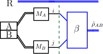 Figure 2
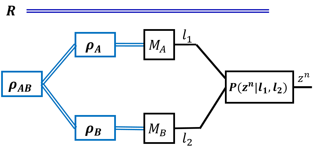 Figure 3
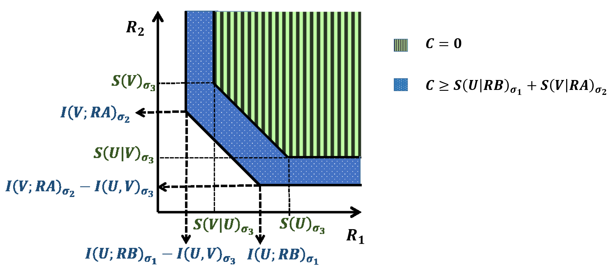 Figure 4
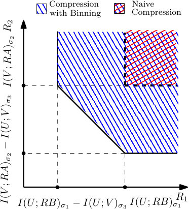 Figure 5
Peer Reviews
No public reviews on file for this paper yet. If you reviewed it on a platform where reviews are public (OpenReview, ICLR, NeurIPS, ICML), you can paste yours below so the community can read it here.
Videos
No videos yet. Explain this paper in a talk, walkthrough, or lecture? Add one.
Faithful Simulation of Distributed Quantum Measurements with Applications in Distributed Rate-Distortion Theory
Touheed Anwar Atif 1, Mohsen Heidari 2 and S. Sandeep Pradhan 1,
1 EECS Dept., University of Michigan, Ann Arbor, MI.
2 CS Dept., Purdue University, West Lafayette, IN.
1{touheed, pradhanv}@umich.edu, [email protected] This work was presented in part at IEEE International Symposium on Information Theory (ISIT) 2019.
Abstract
We consider the task of faithfully simulating a distributed quantum measurement, wherein we provide a protocol for the three parties, Alice, Bob and Eve, to simulate a repeated action of a distributed quantum measurement using a pair of non-product approximating measurements by Alice and Bob, followed by a stochastic mapping at Eve. The objective of the protocol is to utilize minimum resources, in terms of classical bits needed by Alice and Bob to communicate their measurement outcomes to Eve, and the common randomness shared among the three parties, while faithfully simulating independent repeated instances of the original measurement. To achieve this, we develop a mutual covering lemma and a technique for random binning of distributed quantum measurements, and, in turn, characterize a set of sufficient communication and common randomness rates required for asymptotic simulatability in terms of single-letter quantum information quantities. Furthermore, using these results we address a distributed quantum rate-distortion problem, where we characterize the achievable rate distortion region through a single-letter inner bound. Finally, via a technique of single-letterization of multi-letter quantum information quantities, we provide an outer bound for the rate-distortion region.
Contents
-
III Simulation of Distributed POVMs with Deterministic Processing
-
VII Simulation of Distributed POVMs with Stochastic Processing
I Introduction
Measurements interface the intricate quantum world with the perceivable macroscopic classical world by associating a classical attribute to a quantum state. However, quantum phenomena, such as superposition, entanglement and non-commutativity contribute to uncertainty in the measurement outcomes. A key concern, from an information-theoretic standpoint, is to quantify the amount of “relevant information” conveyed by a measurement about a quantum state.
Winter’s measurement compression theorem [1] (also elaborated in [2]) quantifies the “relevant information” as the amount of resources needed to simulate the output of a quantum measurement applied on a given state in an asymptotic sense. Imagine that an agent (Alice) performs a measurement on a quantum state , and sends a set of classical bits to a receiver (Bob). Bob intends to faithfully recover the outcomes of Alice’s measurements without having access to . The measurement compression theorem states that at least quantum mutual information () amount of classical information and conditional entropy () amount of common shared randomness are needed to obtain a* faithful simulation*, where denotes a reference of the quantum state, and denotes the auxiliary register corresponding to the random measurement outcome. Wilde et al. [2] extended the measurement compression problem by considering additional resources available to each of the participating parties. One such formulation allows Bob to further process the information received from Alice using local private randomness. In analogy with [3], this problem formulation is referred to as non-feedback measurement simulation, while the former is termed as simulation with feedback. This quantified the benefit of private randomness in terms of enhancing the trade-off between classical bits communicated and common random bits consumed. In particular, the use of private randomness increases the requirement of classical communication bits, while reducing the common randomness constraint.
The measurement compression theorem finds applications in several paradigms including local purity distillation [2] and private classical communication over quantum channels [4]. This theorem was later used by Datta, et al. [5] to develop a quantum-to-classical (q-c) rate-distortion theory. The problem involved lossy compression of a quantum information source into classical bits, with the task of compression performed by applying a measurement on the source. In this problem, the objective is to minimize the storage of the classical outputs resulting from the measurement, while being able to recover the quantum state (from classical bits) within a fixed level of distortion as measured by an observable. To achieve this, the authors in [6] advocated the use of measurement compression protocol, and subsequently characterized the so-called rate-distortion function in terms of single-letter quantum mutual information quantities. The authors further established that by employing a naive approach of measuring individual output of the quantum source, and then applying Shannon’s rate-distortion theory to compress the classical data obtained is insufficient to achieve optimal rates. Further, the problem of measurement compression in the presence of quantum side information was studied in [2]. The authors here combined the ideas from [1] and [7] to reduce the classical communication rate and common randomness needed to simulate a measurement in presence of quantum side information. Recently, authors in [8] came up with a completely different technique for analyzing the measurement simulation protocols, while considering the problem of quantum measurement compression with side information. They provide a protocol based on convex-split and position based decoding, and bound rates from above in terms of smooth max and hypothesis testing relative entropies (defined in [8]).
In this work, we consider scenarios where the quantum measurements are performed in a distributed fashion on bipartite entangled states, and quantify “relevant information” for these distributed quantum measurements in an asymptotic sense. As shown in Fig. 1, a composite bipartite quantum system is made available to two agents, Alice and Bob, where they have access to the sub-systems and , respectively. Two separate measurements, one for each sub-system, are performed in a distributed fashion with no communication taking place between Alice and Bob. Imagine that there is a third party, Eve, who is connected to Alice and Bob via two separate classical links. The objective of the three parties is to simulate the action of repeated independent measurements performed on many independent copies of the given composite state. To achieve this objective, Alice and Bob send classical bits to Eve at rate and , respectively. Further, common randomness at rate is also shared amidst the three parties. Eve performs classical processing of the received bits and common randomness. We study two settings, based on whether or not Eve has access to private randomness. As an application of this quantification, we consider the quantum-to-classical distributed rate distortion problem where Eve is allowed to use classical-to-quantum channels. In this work, we focus on memoryless quantum systems in finite dimensional Hilbert spaces. We summarize the contributions of this work in the following:
- •
We formulate the problem of faithful simulation of distributed quantum measurements that can be decomposed as a convex-linear combination (incorporating Eve’s stochastic processing) of separable measurements, as stated in Definition 1. The asymptotic performance limit for this problem is given by the set of all communication rates and all common randomness rates , referred to as the achievable rate region, under which the above-stated measurement is distributively simulated. We devise a distributed simulation protocol for this problem, and provide a quantum-information theoretic inner bound to the achievable rate region in terms of computable single-letter information quantities (see Theorem 6). This is the first main result of the paper.
- •
As an immediate application of our results on the simulation of distributed measurements, we develop an approach for a distributed quantum-to-classical rate distortion theory, where the objective is to reconstruct a quantum state at Eve, with the quality of reconstruction measured using an additive distortion observable. The asymptotic performance limit is given by the set of all communication rate pairs at which the distortion is achieved. For the achievability part, we characterize an inner bound in terms of single-letter quantum mutual information quantities (see Theorem 3). This is the second main result of the paper. The classical version of this result is called the Berger-Tung inner bound [9].
- •
We then develop a technique for deriving converse bounds based on a combination of tensor-product and direct-sum Hilbert spaces (also referred to as a multi-particle system). Using this technique, we derive a single-letter outer-bound on the optimal rate distortion region (see Theorem 4), by converting a multi-letter expression into a single-letter expression. This is the third main result of the paper.
The organization of the paper is as follows. In Section II, we set the notation and state requisite definitions. Instead of first presenting the above-stated inner bound to the performance limits of the problem of simulation of distributed measurements in its full generality, for pedagogical reasons, in Section III, we first consider a special case, where the processing at Eve is restricted to a deterministic function, and provide a simple proof based on the application of Winter’s measurement compression theorem. In this setup, we compress each individual measurements and , comprising the decomposing of . As a result, faithful simulation of is possible when at least classical bits of communication and bits of common randomness are available between Alice and Eve. Similarly, a faithful simulation of is possible with classical bits of communication and bits of common randomness between Eve and Bob, where and are purifications of the sub-systems and , respectively, and and denote the auxiliary registers corresponding to their measurement outcomes. The challenge here is that the direct use of single-POVM compression theorem for each individual POVMs, and , does not necessarily ensure a “distributed” faithful simulation of the overall measurement, . To accomplish this, we develop a Mutual Covering Lemma (see Lemma 4), which also helps in converting the information quantities in terms of the reference of the joint state .
Further, an interesting aspect about the distributed setting is that one can further reduce the amount of classical communication by exploiting the statistical correlations between Alice’s and Bob’s measurement outcomes. The challenge here is that the classical outputs of the approximating POVMs (operating on copies of the state ) are not independent identically distributed (IID) sequences — rather they are codewords generated from random coding. For this we develop a proposition for mutual packing (Proposition 2), that characterizes the binning rates in term of single-letter information quantities. This issue also arises in classical distributed source coding problem which was addressed by Wyner-Ahlswede-Körner [9] by developing Markov lemma and Mutual packing lemma. The idea of binning in quantum setting has been explored from a different perspective in [10] and [11] for quantum data compression involving side information. Toward the end of the section, we also provide an example to illustrate the inner bound to the achievable rate region.
In Section V, we apply this special setting of the distributed measurement simulation with deterministic processing to the q-c distributed rate distortion problem. Since, the proof of the inner bound of this rate distortion problem requires only the special case of distributed measurement simulation, this is another reason for providing the special case in the previous section.
In Section VI, we consider the non-feedback measurement compression problem for the point-to-point setting. The authors in [2] have discussed this formulation and provided a rate region with a proof of achievability and converse. However, the assumed equations (53) and (54) in proving the direct part (see [2]) do not appear to be true, to the best to our knowledge, but only in an average sense. A stronger version of this theorem is also developed in [12] using a different technique, wherein the authors have extended the Winter’s measurement compression for fixed independent and identically distributed inputs [1] to arbitrary inputs. Since the result is crucial for the distributed simulation problem with stochastic processing, to be described in the next section (Section VII), we formally state the problem and provide an alternative proof of the direct part for completeness (see Theorem 5).
Finally, the above proof of non-feedback simulation in the point-to-point setting provides us with necessary tools for the next task, namely, distributed quantum measurement simulation with stochastic processing. The objective of incorporating the additional processing at the decoder is to reduce the required shared randomness. Our objective in the distributed problem, considered in Section III, was to simulate . We achieve this by proving that a pair of POVMs that can faithfully simulate and individually, can also faithfully simulate (Lemma 4). However, it will be shown that, because of the presence of Eve’s stochastic processing, decoupling the current problem into two symmetric point-to-point problems is not feasible. Therefore, we perform a non-symmetric partitioning while being analytically tractable. Moreover, we provide a single-letter achievable inner bound that is symmetric with respect to Alice and Bob. We conclude the paper with a few remarks in Section IX.
II Preliminaries
We here establish all our notations, briefly state few necessary definitions, and also provide Winter’s theorem on measurement compression.
Notation: Given any natural number , let the finite set be denoted by . Let denote the algebra of all bounded linear operators acting on a finite dimensional Hilbert space . Further, let denote the set of all unit trace positive operators acting on . Let denote the identity operator. The trace distance between two operators and is defined as , where for any operator we define . The von Neumann entropy of a density operator is denoted by . The quantum mutual information for a bipartite density operator is defined as
[TABLE]
Given any ensemble , the Holevo information, as in [13], is defined as
[TABLE]
A positive-operator valued measure (POVM) acting on a Hilbert space is a collection of positive operators in that form a resolution of the identity:
[TABLE]
where is a finite set. If instead of the equality above, the inequality holds, then the collection is said to be a sub-POVM. A sub-POVM can be completed to form a POVM, denoted by , by adding the operator to the collection. Let denote a purification of a density operator . Given a POVM acting on , the post-measurement state of the reference together with the classical outputs is represented by
[TABLE]
Consider two POVMs and acting on and , respectively. Define With this definition, is a POVM acting on . By denote the -fold tensor product of the POVM with itself.
Definition 1** (Joint Measurements).**
A POVM , acting on the joint state , is said to have a separable decomposition with stochastic integration if there exist POVMs and and a stochastic mapping such that
[TABLE]
where and are some finite sets. Further, if the mapping is a deterministic function then the POVM is said to have a separable decomposition with deterministic integration.
Measurement Compression Theorem: Here, we provide a brief overview of the measurement compression theorem [1]. A key concern, from an information-theoretic standpoint, is to quantify the amount of “relevant information” conveyed by a measurement about a quantum state. Winter quantified “relevant information” by measuring the minimum amount of classical information bits needed to “simulate” the repeated action of a measurement on a quantum state . In this context, an agent (Alice) performs an approximating measurement on a quantum state and sends a set of classical bits to a receiver (Bob). In addition, Alice and Bob share some amount of common randomness. Bob intends to faithfully recover the outcomes of the original measurement without having access to the quantum state based on the bits received from Alice and the common randomness. The objective is to minimize the rate of classical bits under the constraint that the recovered and the original outcomes be statistically indistinguishable. This is formally defined in the following.
Definition 2** (Faithful simulation [2]).**
Given a POVM acting on a Hilbert space and a density operator , a sub-POVM acting on is said to be -faithful to with respect to , for , if the following holds:
[TABLE]
The above trace norm constraint can be equivalently expressed in terms of a purification of state using the following lemma.
Lemma 1**.**
[2]* For any state with any purification , and any pair of POVMs and acting on , the following identity holds*
[TABLE]
where and are the operators associated with and , respectively.
Theorem 1**.**
[1]* For any , any density operator and any POVM acting on the Hilbert space , there exist a collection of POVMs for , each acting on , and having at most outcomes such that is -faithful to with respect to if*
[TABLE]
where , and as .
Remark 1**.**
A strong converse of the above result is also provided in [1].
III Simulation of Distributed POVMs with Deterministic Processing
Now, we develop an extension of Winter’s measurement compression [1] to quantum measurements performed in a distributed fashion with deterministic processing. Consider a bipartite composite quantum system represented by Hilbert Space . Let be a density operator on . Consider two measurements and on sub-systems and , respectively. Imagine that three parties, named Alice, Bob and Eve, are trying to collectively simulate these two measurements, one applied to each sub-system. The three parties share some amount of common randomness. Alice and Bob perform a measurement and on copies of sub-systems and , respectively. The measurements are performed in a distributed fashion with no communication taking place between Alice and Bob. Based on their respective measurements and the common randomness, Alice and Bob send some classical bits to Eve. Upon receiving these classical bits, Eve applies a processing operation on them and then wishes to produce an -letter classical sequence. The objective is to construct -letter measurements and that minimize the classical communication and common randomness bits while ensuring that the overall measurement induced by the action of the three parties is close to . The problem is formally defined in the following.
Definition 3**.**
For a given finite set , and a Hilbert space , a distributed protocol with parameters is characterized by
1) a collections of Alice’s sub-POVMs each acting on and with outcomes in a subset satisfying .
2) a collections of Bob’s sub-POVMs each acting on and with outcomes in a subset , satisfying .
3) a collection of Eve’s decoding maps for .
The overall sub-POVM of this distributed protocol, given by , is characterized by the following operators:
[TABLE]
where and are the operators corresponding to the sub-POVMs and , respectively.
In the above definition, determines the amount of classical bits communicated from Alice and Bob to Eve. The amount of common randomness is characterized by , and can be viewed as the common randomness bits distributed among the parties. The mapping represents the action of Eve on the received classical bits.
Definition 4**.**
Given a POVM acting on , and a density operator , a triplet is said to be achievable, if for all and for all sufficiently large , there exists a distributed protocol with parameters such that its overall sub-POVM is -faithful to with respect to (see Definition 2), and
[TABLE]
The set of all achievable triples is called the achievable rate region.
The following theorem provides an inner bound to the achievable rate region, which is proved in Section IV,
Theorem 2**.**
Given a density operator and a POVM acting on having a separable decomposition with deterministic integration (as in Definition 1), a triple is achievable if the following inequalities are satisfied:
[TABLE]
*for some decomposition with POVMs and and a function , where the information quantities are computed for the auxiliary states and , with being a purification of , and and are some finite sets. *
Remark 2**.**
An alternative characterization of the above rate region can be obtained in terms of Holevo information. For this, we use the canonical ensembles , and defined as
[TABLE]
Using this, we get
[TABLE]
Also, , and are equal to the classical mutual information and joint entropy with respect to the joint distribution , respectively.
Before providing a proof in the next section, we briefly discuss two corner points of the rate region with respect to the common randomness available. Firstly, consider the regime where the sum rate is at its minimum achievable, i.e., equation (5c) is active. This requires the largest amount of common randomness, given by the constraint . Next, let us consider the regime where . This implies . This regime corresponds to the quantum measurement followed by classical Slepian-Wolf compression [14]. Fig. 2 demonstrates the achievable rate region in these cases.
We encounter two challenges in developing the single-letter inner bound to the achievable rate region as stated in Theorem 2:
-
The direct use of single-POVM compression theorem, proved using random coding arguments as in [1], for each individual POVMs, and , does not necessarily ensure a “distributed” faithful simulation for the overall measurement, . This issue is unique to the quantum settings. One of the contributions of this work is to prove this when the two sources and are not necessarily independent, i.e., (see Lemma 4).
-
The classical outputs of the approximating POVMs (operating on copies of the source) are not independently and identically distributed (IID) sequences - rather they are codewords generated from random coding. The Slepian-Wolf scheme [14] (also referred to as binning in the literature) is developed for distributed compression of IID source sequences. Applicability of such an approach to the problem requires that the classical outputs produced from the two approximating POVMs are jointly typical with high probability. This issue also arises in classical distributed source coding problem which was addressed by Wyner-Ahlswede-Korner by developing Markov Lemma and Mutual Packing Lemma (Lemma 12.1 and 12.2 in [15]). Building upon these ideas, we develop quantum-classical counterparts of these lemmas for the multi-user quantum measurement simulation problem (see the discussion in Section IV-B and Proposition 2). Let us consider an example to illustrate the above inner bound.
Example 1**.**
Suppose the composite state is described using one of the Bell states on as
[TABLE]
Since and , Alice and Bob would perceive each of their particles in maximally mixed states and , respectively. Upon receiving the quantum state, the two parties wish to independently measure their states, using identical POVMs and , given by . Alice and Bob together with Eve are trying to simulate the action of using the classical communication and common randomness as the resources available to them (as described earlier).
We compute the constraints given in Theorem 2. Considering the first constraint from , we evaluate as
[TABLE]
where the vectors denote a set of orthogonal states on the space . Based on this state, we get
[TABLE]
This gives to be equal to 1 bit. Similarly, from the symmetry of the example, we also get to be equal to 1 bit. Similarly, we can evaluate as
[TABLE]
which gives
[TABLE]
Therefore, we can write the constraints given in Theorem 2 as
[TABLE]
Consider the case when is available. By approximating and individually, we receive a gain of 1 bit, decreasing the rate from bits to bit and similarly from bits to bit. Binning of these approximating POVMs (as discussed in Section (IV-B)), gives an additional gain of half a bit, which is characterized by , thus giving us the achievable sum-rate of bits.
In the next section we provide the proof for this inner bound.
IV Proof of Theorem 2
Assume that the operators of the original POVM are decomposed as
[TABLE]
for some POVMs and with operators denoted by and , respectively, and for some function where and are three finite sets. The proof follows by constructing a protocol for faithful simulation of . We start by generating the canonical ensembles corresponding to and , as given in (2). With this notation, corresponding to each of the probability distributions, we can associate a -typical set. Let us denote , and as the -typical sets defined for , and , respectively.
Let and denote the -typical projectors (as in [13]) for marginal density operators and , respectively. Also, for any and , let and denote the conditional typical projectors (as in [13]) for the canonical ensembles and , respectively. For each and define
[TABLE]
where and 111Note that and are not tensor products operators..
With the notation above, define and as
[TABLE]
where and . Note that and defined above are expectations with respect to the pruned distribution [16]. Let and be the projectors onto the subspaces spanned by the eigen-states of and corresponding to eigenvalues that are larger than and , for some . Lastly, define222Note that and are not tensor products operators..
[TABLE]
IV-A Construction of Random POVMs
In what follows, we construct two random POVMs one for each encoder. Fix a positive integer and positive real numbers and satisfying and , where is defined as
[TABLE]
with being any purification of 333The information theoretic quantities calculated with respect to remain independent of the purification used in its definition.. Let denote the common randomness shared between the first encoder and the decoder, and let denote the common randomness shared between the second encoder and the decoder, with log() + log() log(). For each and , randomly and independently select and sequences according to the pruned distributions, i.e.,
[TABLE]
Construct operators
[TABLE]
where
[TABLE]
where is a parameter to be determined. Then, for each and , construct and as in the following
[TABLE]
We show in the later part of the proof (Lemma 2) that and form sub-POVMs, with high probability, for all and , respectively. These collections and are completed using the operators and , and these operators are associated with sequences and , which are chosen arbitrarily from and , respectively.
IV-B Binning of POVMs
We introduce the quantum counterpart of the so-called binning technique which has been widely used in the context of classical distributed source coding. Fix binning rates and choose a pair. For each sequence assign an index from randomly and uniformly, such that the assignments for different sequences are done independently. Perform a similar random and independent assignment for all with indices chosen from . Repeat this assignment for every and . For each and , let and denote the and the bins, respectively. More precisely, is the set of all sequences with assigned index equal to , and similar is . Define the following operators:
[TABLE]
for all and . Using these operators, we form the following collection:
[TABLE]
Note that if and are sub-POVMs, then so are and . This is due to the relations
[TABLE]
To make and complete, we define and as and , respectively444Note that and . Now, we intend to use the completions and as the POVMs for each encoder. Also, note that the effect of the binning is in reducing the communication rates from to .
IV-C *Decoder mapping *
Note that the operators are used to simulate . Binning can be viewed as partitioning of the set of classical outcomes into bins. Suppose an outcome occurred after the measurement. Then, if the bins are small enough, one might be able to recover the outcomes by knowing the bin numbers. For that we create a decoder that takes as an input a pair of bin numbers and produces a pair of sequences . More precisely, we define a mapping , for , acting on the outputs of as follows. Let denote the codebook containing all pairs of codewords . On observing and the classical indices communicated by the encoder, the decoder first deduces from and then populates,
[TABLE]
For every , and define the function if is the only element of ; otherwise Further, for or . Finally, the decoder produces according to the map . With this mapping, we form the following collection of operators, denoted by ,
[TABLE]
Note that for for (u^{n},v^{n})\notin(\mathcal{T}_{\delta}^{(n)}(U)\times\mathcal{T}_{\delta}^{(n)}(V))\operatorname*{\mathbin{\scalebox{1.0}{\bigcup}}}\{(u^{n}_{0},v^{n}_{0})\}. We show that is a POVM that is -faithful to the intermediate POVM , with respect to . For faithful simulation of the original POVM , we apply the deterministic mapping to the classical outputs of . More precisely, we construct the POVM with the following operators:
[TABLE]
IV-D Analysis of POVM and Trace Distance
In what follows, we show that is a POVM, and is -faithful with respect to (according to Definition 2) to , where can be made arbitrarily small for sufficiently large . More precisely, we show that, with probability sufficiently close to 1,
[TABLE]
According to the decomposition of , given in (7), the above inequality is equivalent to
[TABLE]
From triangle inequality, the left-hand side of the above inequality does not exceed the following
[TABLE]
Hence, it is sufficient to show that the above quantity is no greater than , with probability sufficiently close to 1. This is equivalent to showing that is -faithful to with respect to . Alternatively, using Lemma 1, we prove the following inequality
[TABLE]
We characterize the conditions on under which the inequality given in (20) holds, using the following steps.
**Step 1: and are sub-POVMs and individually approximating
**As a first step, one can show that with probability sufficiently close to one, and form sub-POVMs for all and , and also individually approximate the corresponding tensor product POVMs. More precisely the following Lemma holds.
Lemma 2**.**
For any two positive integers and , and , as in (15), and any , there exists such that for all , the collection of operators and form sub-POVMs for all and with probability at least , provided that
[TABLE]
where are defined as in the statement of the theorem. In addition, if
[TABLE]
*then with probability at least the collection of average operators are -faithful to with respect to and with respect to , respectively. *
Proof.
The proof uses a similar argument as in that of Theorem 2 in [1]. Hence it is omitted. ∎
As a result of the lemma, and are valid POVMs with high probability.
**Step 2: Isolating the effect of un-binned approximating measurements
**In this step, we separate out the effect of un-binned approximating measurements from in (20). This is done by adding and subtracting an appropriate term within the trace norm and applying triangle inequality, which bounds as , where
[TABLE]
where the captures the effect of using approximating POVMs and instead of the actual POVMs and , while captures the error introduced by binning these approximating POVMs. Before we proceed further, we provide the following lemma which will be useful in the rest of the paper.
Lemma 3**.**
Given a density operator , a sub-POVM acting on for some set , and any Hermitian operator acting on , we have
[TABLE]
with equality if , where .
Proof.
The proof is provided in Appendix A-A. ∎
Next, we show is sufficiently small using the following Mutual Covering Lemma.
Lemma 4** (Mutual Covering Lemma).**
Suppose the sub-POVM is -faithful to with respect to , and the sub-POVM is -faithful to with respect to , where and . Then the sub-POVM is -faithful to the POVM with respect to .
Proof.
The proof is provided in the Appendix A-B. ∎
Using Lemma 4 with , , , and , and Lemma 2, with probability at least , we have .
**Step 3: Analyzing the effect of Binning
**In this step, we provide an upper bound on . For , define . For any define . Note that captures the overall effect of the binning followed by the decoding function . For all and , let . With this notation, we simplify using the following proposition.
Proposition 1**.**
* can be simplified as*
[TABLE]
where is defined as
[TABLE]
Proof.
The proof is provided in Appendix B-A. ∎
In the next proposition we provide a bound on .
Proposition 2** (Mutual Packing).**
There exist functions and , such that for all sufficiently small and sufficiently large , we have , if , where is the auxiliary state defined in the theorem and as .
Proof.
The proof is provided in Appendix B-B. ∎
Using this, and from Step 2, with probability sufficiently close to one, we have
[TABLE]
IV-E Rate Constraints
To sum-up, we showed that the trace distance inequality in (20) holds for sufficiently large and with probability sufficiently close to 1, if the following bounds hold:
[TABLE]
where for . This implies that is -faithful to with probability sufficiently close to one, and hence, is also -faithful to with respect to , i.e, (19) is satisfied. Therefore, there exists a distributed protocol with parameters such that its overall POVM is -faithful to with respect to . Lastly, we complete the proof of the theorem using the following lemma.
Lemma 5**.**
Let denote the set of all for which there exists such that the sextuple satisfies the inequalities in (24). Let, denote the set of all triples that satisfies the inequalities in (5) given in the statement of the theorem. Then, .
Proof.
The prove follows by Fourier-Motzkin elimination [17]. ∎
V Q-C Distributed Rate Distortion Theory
As an application of faithful simulation of distributed measurements (Theorem 2), we consider the distributed extension of q-c rate distortion coding [5]. This problem is a quantum counterpart of the classical distributed source coding. In this setting, consider a memoryless bipartite quantum source, characterized by . Alice and Bob have access to sub-systems and , characterized by and , respectively, where and . They both perform a measurement on copies of their sub-systems and send the classical bits to Eve. Upon receiving the classical bits sent by Alice and Bob, a reconstruction state is produced by Eve. The objective of Eve is to produce a reconstruction of the source within a targeted distortion threshold which is measured by a given distortion observable.
V-A Problem Formulation
We first formulate this problem as follows. For any quantum information source, characterized by , denote its purification by .
Definition 5**.**
A q-c source coding setup is characterized by a triple , where is a purified quantum state, is a reconstruction Hilbert space, and , which satisfies , is a distortion observable.
Next, we formulate the action of Alice, Bob and Eve by the following definition.
Definition 6**.**
An q-c protocol for a given input and reconstruction Hilbert spaces is defined by POVMs and acting on and with and number of outcomes, respectively, and a set of reconstruction states for all .
The overall action of Alice, Bob and Eve, as a q-c protocol, on a quantum source is given by the following operation
[TABLE]
where and are the operators of the POVMs and , respectively. With this notation and given a q-c source coding setup as in Definition 5, the distortion of a q-c protocol is measured as
[TABLE]
For an -letter protocol, we use symbol-wise average distortion observable defined as
[TABLE]
where is understood as the observable acting on the th instance space of the -letter space . With this notation, the distortion for an q-c protocol is given by
[TABLE]
where is the -fold tensor product of which is the given purification of the source.
The authors in [5] studied the point-to-point version of the above formulation. They considered a special distortion observable of the form where acts on the reference Hilbert space and is the reconstruction alphabet. In this paper, we allow to be any non-negative and bounded operator acting on the appropriate Hilbert spaces. Moreover, we allow for the use of any c-q reconstruction mapping as the action of Eve.
Definition 7**.**
For a q-c source coding setup , a rate-distortion triplet () is said to be achievable, if for all and all sufficiently large , there exists an q-c protocol satisfying
[TABLE]
where is defined as in (25). The set of all achievable rate-distortion triplets is called the achievable rate-distortion region.
Our objective is to characterize the achievable rate-distortion region using single-letter information quantities.
V-B Inner Bound
We provide an inner bound to the achievable rate-distortion region which is stated in the following theorem. We employ a q-c protocol based on a randomized faithful simulation strategy involving a time sharing classical random variable that is independent of the quantum source. This can be viewed as a conditional version of the faithful simulation problem considered in Section III.
Theorem 3**.**
For a q-c source coding setup , any rate-distortion triplet satisfying the following inequalities is achievable
[TABLE]
for POVM of the form , where for every , and are POVMs acting on , and reconstruction states with each state in , and some finite sets and . The quantum mutual information quantities are computed according to the auxiliary states and where represents the output of , and .
Remark 3**.**
Note that for the auxiliary states , we have .
Proof.
In the interest of brevity, we provide the proof for the special case, when the time sharing random variable is trivial, i.e., is empty. An extension to the more general case is straightforward but tedious. For the special case, the proof follows from Theorem 2. Fix POVMs and reconstruction states as in the statement of the theorem. Let be the mapping corresponding to these POVMs and the reconstruction states. Then, According to Theorem 2, for any , there exists an distributed protocol for -faithful simulation of with respect to such that satisfies the inequalities in (5) for and . Let and be the POVMs and the deterministic decoding functions of this protocol with . We use these POVM’s and mappings to construct a q-c protocol for distributed quantum source coding.
For each , consider the q-c protocol with parameters , and POVMs . Moreover, we use n-length reconstruction states S_{i,j}\mathrel{\ensurestackMath{\stackon[1pt]{=}{\scriptstyle\Delta}}}\sum_{u^{n},v^{n}}\mathbbm{1}\big{\{}f^{(\mu)}(i,j)=(u^{n},v^{n})\big{\}}S_{u^{n},v^{n}}, where . Further, let the corresponding mappings be denoted as . With this notation, for the average of these random protocols, the following bounds hold:
[TABLE]
where is the average of , and is the overall POVM of the underlying distributed protocol as given in (4). The first inequality holds by the fact that . The second inequality follows by Lemma 6 given in the sequel. The third inequality is due to the monotonicity of the trace-distance [16] with respect to the quantum channel given by , where
[TABLE]
The last inequality follows by Theorem 2, and the fact that . This completes the proof of the theorem, since is a bounded operator. ∎
Lemma 6**.**
For any operator and acting on a Hilbert space the following inequalities hold.
[TABLE]
Proof.
See Exercise 12.2.1 in [16]. ∎
One can observe that the rate region in Theorem 3 matches in form with the classical Berger-Tung region when is a mixed state of a collection of orthogonal pure states. Note that the rate region is an inner bound for the set of all achievable rates. The single-letter characterization of the set of achievable rates is still an open problem even in the classical setting. Some progress has been made recently on this problem which provides an improvement over Berger-Tung rate region [18].
V-C Outer Bound
In this section, we provide an outer bound for the achievable rate-distortion region.
Theorem 4**.**
Given a q-c source coding setup , if any triplet is achievable, then the following inequalities must be satisfied
[TABLE]
for some state which can be written as
[TABLE]
*where represents an auxiliary quantum state, and is a quantum test channel with . *
Proof.
Suppose the triplet is achievable. Then, from Definition 7, for all , there exists an q-c protocol satisfying the inequalities in the definition. Let , and be the corresponding POVMs and reconstruction states. Let denote the outcomes of the measurements. Then, for Alice’s rate, we obtain
[TABLE]
where the state is defined as
[TABLE]
Note that for each the corresponding mutual information above is defined for a state in the Hilbert space . Next, we convert the above summation into a single-letter quantum mutual information term. For that we proceed with defining a new Hilbert space using direct-sum operation.
Let us recall the direct-sum of Hilbert spaces [19]. Consider a tuple of Hilbert spaces , with inner products . Define as the collection of tuples of vectors . The inner product of two tuples and is given by the sum of inner products of the components, i.e., . A linear operator in this space is a tuple of operators given by , where operates on , and . A state in is denoted conventionally as . Similarly, a linear operator in this space is written in the form .
With this definition, consider the following single-letterization:
[TABLE]
where the state is defined below
[TABLE]
where denotes tracing over , and , and is an averaging random variable which is uniformly distributed over . We elaborate on the Hilbert space associated with as follows.
Suppose is an orthonormal basis for . Then, a basis for is given by
[TABLE]
for all . Consider the direct-sum of the Hilbert spaces . Consider the Hilbert space . With this definition, define , as the Hilbert space which is spanned by for all and . Therefore, is isometrically isomorphic to the direct-sum . Note that can be viewed as a multi-particle Hilbert space, which is a truncated version of the so-called Fock space [20].
Similarly, for Bob’s rate we have
[TABLE]
For the sum-rate, the following inequalities hold
[TABLE]
In addition, the distortion of this q-c protocol satisfies , where is the quantum channel associated with the protocol. Therefore, as the distortion observable is symbol-wise additive, we obtain
[TABLE]
where the third equality holds, because of the following argument. From (V-C), one can show by partially tracing over , that
[TABLE]
and I_{Q}\mathrel{\ensurestackMath{\stackon[1pt]{=}{\scriptstyle\Delta}}}\bigoplus_{j=1}^{n}\big{(}I_{R}^{\otimes(j-1)}\otimes\outerproduct{j}{j}\big{)}. Then, is the identity operator acting on . Therefore, the right-hand side of the equality above can be written as
[TABLE]
Let us identify the single-letter quantum test channel as given in the statement of the theorem. First, due to the distributive property of tensor product over direct sum operation, we can rewrite as
[TABLE]
Next, we identify a quantum channel . For that and for any define the following intermediate quantum channels:
[TABLE]
where . One can verify that is indeed a quantum channel. With these definitions, let
[TABLE]
Using the property of direct-sum operation, one can verify that is a valid quantum channel, moreover,
[TABLE]
Lastly, we show that the condition is also satisfied. By taking the partial trace of over we obtain the following state
[TABLE]
where the last equality is due to the distributive property of tensor product over direct sum operation. Hence, is in a tensor product of the form , and therefore, .
Remark 4**.**
One may question the computability of the outer bound provided in Theorem 4. The computability of this bound depends on the dimensionality of the auxiliary space defined in the theorem. Currently, we are unable to bound the dimension of the Hilbert space , but aim to provide one in our future work. As a matter of fact, the current outer bounds for the equivalent classical distributed rate distortion problem still suffers from the computability issue. The first outer bound to the classical problem was provided in [9] and a recent substantial improvement was made by authors in [21]. Both of these bounds suffer from the absence of cardinality bounds on at least one of the variables used and hence cannot be claimed to be computable using finite resources.
∎
VI Simulation of POVMs with Stochastic Processing
We now provide an extension of the Winter’s point-to-point measurement compression scheme [1] (discussed in Section 1) with stochastic processing. We assume that the receiver (Bob) has access to additional private randomness, and he is allowed to use this additional resource to perform any stochastic mapping of the received classical bits. In fact, the overall effect on the quantum state can be assumed to be a measurement which is a concatenation of the POVM Alice performs and the stochastic map Bob implements. Hence, Alice in this case, does not remain aware of the measurement outcome. It is for this reason that [2] describes this as a non-feedback problem, with the sender not required to know the outcomes of the measurement. With the availability of additional resources, such a formulation is expected to help reduce the overall resources needed.
VI-A Problem Formulation
Definition 8**.**
For a given finite set , and a Hilbert space , a measurement simulation protocol with stochastic processing with parameters is characterized by
1) a collections of Alice’s sub-POVMs each acting on and with outcomes in a subset satisfying .
2) a Bob’s classical stochastic map for all , and .
The overall sub-POVM of this distributed protocol, given by , is characterized by the following operators:
[TABLE]
where are the operators corresponding to the sub-POVMs .
In the above definition, characterizes the amount of classical bits communicated from Alice to Bob, and the amount of common randomness is determined by , with being the common randomness bits distributed among the parties. The classical stochastic mappings induced by represents the action of Bob on the received classical bits.
Definition 9**.**
Given a POVM acting on , and a density operator , a pair is said to be achievable, if for all and for all sufficiently large , there exists a measurement simulation protocol with stochastic processing with parameters such that its overall sub-POVM is -faithful to with respect to (see Definition 2), and
[TABLE]
The set of all achievable pairs is called the achievable rate region.
The following theorem characterizes the achievable rate region.
Theorem 5**.**
For any density operator and any POVM acting on the Hilbert space , a pair is achievable if and only if there exist a POVM , with being a finite set, and a stochastic map such that
[TABLE]
*where *
Remark 5**.**
An alternative characterization of the above rate region can also be obtained in terms of Holevo information. For this, we define the following ensemble as
[TABLE]
for being the canonical ensemble associated with the POVM and the state as defined in (2). With this ensemble, we have
[TABLE]
VI-B Proof of Achievability of Theorem 5
Suppose there exist a POVM and a stochastic map , such that can be decomposed as
[TABLE]
We begin by defining a canonical ensemble corresponding to as where
[TABLE]
Similarly. for each , we also define
[TABLE]
where , and and are similar to the ones defined in Section IV. Using the above definitions, we now construct the approximating POVM.
VI-B1 Construction of Random POVMs
In what follows, we construct a collection of random POVMs. Fix and as two positive integers. Let denote the common randomness shared between the sender and receiver. For each , randomly and independently select sequences according to the pruned distributions, i.e.,
[TABLE]
For , let the operators of the POVM be for each , where is defined as
[TABLE]
with being a parameter to be determined. Now, for each construct as
[TABLE]
Since the construction is very similar to the one used in Section IV, we make a claim similar to the one in Lemma 2. This claim gives us the first constraint on the classical rate of communication , which ensures that the operators constructed above for all are valid sub-POVMs (characterized as the event ) with high probability. The claim is as follows. If then for some ; or in other words, with probability sufficiently close to one, forms a sub-POVM for all . Note the definition of follows from the statement of theorem. From this, let denote the completion of the corresponding sub-POVM for . Let the operators completing these POVMs, given by , be denoted by for some for all , and for w^{n}\notin\mathcal{T}_{\delta}^{(n)}(W)\operatorname*{\mathbin{\scalebox{1.0}{\bigcup}}}\{w_{0}^{n}\}. Using this construction, we define the intermediate POVM as and the operators of as Now, we define Bob’s stochastic map as , yielding the operators of the final approximating POVM as
[TABLE]
VI-B2 Trace Distance
Now, we compare the action of this approximating POVM on the input state with that of the given POVM , using the characterization provided in Definition 2. Specifically, we show using the expressions for canonical ensemble that, with probability close to one,
[TABLE]
As a first step, we split and bound as , where
[TABLE]
Now we bound by adding and subtracting an appropriate term and using triangle inequality as , where and are given by
[TABLE]
Note that in the above expressions, we have used an additional triangle inequality for block operators (which is in fact an equality) to move the summation over inside the trace norm. Firstly, we show is small with high probability. To simplify the notation, we define which gives as
[TABLE]
We develop the following lemma to bound this term.
Lemma 7**.**
Consider an ensemble given by , where is the pruned distribution as defined in (35) and is any tensor product state of the form . Then, for any , , there exists functions and , such that for all sufficiently large , the inequality
[TABLE]
holds with probability greater than , if , where are independent random vectors generated according to the pruned distribution given in (35), and , as , .
Proof.
The proof of the lemma is provided in Appendix A-C ∎
Therefore, using the lemma above, can be made arbitrarily small, for sufficiently large n, with high probability, given the constraints . Secondly, we bound by applying expectation and using Gentle Measurement Lemma [16] as follows,
[TABLE]
where is obtained by using triangle inequality and the linearity of expectation, is obtained by marginalizing over and using the fact that , is obtained by substitution, and finally uses repeated application of the average gentle measurement lemma, by setting with as and, and (see (35) in [2] for details). Finally, we show that the term corresponding to can also be made arbitrarily small. This term can be simplified as follows
[TABLE]
where
[TABLE]
Now, for the first term in (40) we use Lemma 7 and claim that for given any , if
[TABLE]
then the probability of this term being greater than is bounded by for sufficiently large n, where is as defined in the statement of the theorem . Note that the requirements we obtain on were already imposed when claiming the collection of operators forms a sub-POVM. As for the second term in (40) we again use the gentle measurement Lemma and bound its expected value as
[TABLE]
where is defined in (39).
In summary, we have performed the following sequence of steps. Firstly, we argued that forms a valid sub-POVM for all , with high probability, when the rate satisfies . Secondly, we moved onto bounding the trace norm between the states obtained after the action for these approximating POVMs when compared with those obtained from the action of actual POVM , characterized as using Definition 2. As a first step in establishing this bound, we showed that Considering , we used triangle inequality and divided it into two terms: and . Then, using Lemma 7 we showed that for any given , can be made smaller than with high probability if . As for , we showed that it goes to zero in the expected sense using (39). Finally, for the term given by , we bounded this as a sum of two trace norms and given in (40). We showed that its first term can be made smaller than with high probability if for sufficiently large , and the second term was shown to approach zero in expected sense.
Now, using Markov inequality we argue the existence of at least one collection of POVMs that satisfies the statement of the Theorem 5 as follows. Note that is same as . Let be the event defined earlier in the proof. Let us define and as the random variables corresponding to the terms and , respectively. Firstly, if . then . Secondly, from Lemma 7, for all , and for all sufficiently large n, if
[TABLE]
then we have , . Thirdly, from (39) we have . This implies, from the Markov inequality, that
[TABLE]
Using these bounds, we get
[TABLE]
given that we choose Note that , and the inequality in (VI-B2) ensures that there exists a valid collection of sub-POVMs satisfying , with non-vanishing probability. Therefore, using random coding arguments, there exists at least one collection of sub-POVMs with the above construction satisfying the statement of Theorem 5.
VII Simulation of Distributed POVMs with Stochastic Processing
In this section, we develop a stochastic processing variant of the distributed POVM simulation problem described in Section III. Let be a density operator acting on a composite Hilbert Space . Consider two measurements and on sub-systems and , respectively. Imagine again that we have three parties, named Alice, Bob and Eve, that are trying to collectively simulate a given measurement acting on the state , as shown in Fig. 3. In this version of distributed simulation, Eve additionally has access to unlimited private randomness. The problem is defined in the following.
Definition 10**.**
For a given finite set , and a Hilbert space , a distributed protocol with stochastic processing with parameters is characterized by
1) a collections of Alice’s sub-POVMs each acting on and with outcomes in a subset satisfying .
2) a collections of Bob’s sub-POVMs each acting on and with outcomes in a subset , satisfying .
3) Eve’s classical stochastic map for all and .
The overall sub-POVM of this distributed protocol, given by , is characterized by the following operators:
[TABLE]
where and are the operators corresponding to the sub-POVMs and , respectively.
In the above definition, determines the amount of classical bits communicated from Alice and Bob to Eve. The amount of common randomness is determined by . The classical stochastic maps represent the action of Eve on the received classical bits.
Definition 11**.**
Given a POVM acting on , and a density operator , a triple is said to be achievable, if for all and for all sufficiently large , there exists a distributed protocol with stochastic processing with parameters such that its overall sub-POVM is -faithful to with respect to (see Definition 2), and
[TABLE]
The set of all achievable triples is called the achievable rate region.
The following theorem provides an inner bound to the achievable rate region, which is proved in Section VIII.
Theorem 6**.**
*Given a density operator , and a POVM acting on having a separable decomposition with stochastic integration (as in Definition 1), a triple is achievable if the following inequalities are satisfied: *
[TABLE]
for some decomposition with POVMs and and a stochastic map , where is a purification of , and the above information quantities are computed for the auxiliary states and
Remark 6**.**
An alternative characterization of the above rate region can be obtained in terms of Holevo information. For this, we define the following ensemble as
[TABLE]
with , and being the canonical ensembles defined in (2), and for all . With this ensemble, we have , , and
VIII Proof of Theorem 6
VIII-A Construction of POVMs
Suppose there exist POVMs and and a stochastic map , such that can be decomposed as
[TABLE]
Note that the proof technique here is very different to the one used in Section IV for proving Theorem 2. Recall that in Theorem 2 we initiated the proof by constructing a protocol to faithfully simulate . However, here we are not interested in faithfully simulating . Instead, by carefully exploiting the private randomness Eve possesses, manifested in terms of the stochastic processing applied by her on the classical bits received, i.e., , we aim to strictly reduce the sum rate constraints compared to the ones obtained in (5f) of Theorem 2. This requires a considerably different methodology. More specifically, Lemma 1 was employed in Theorem 2, which guaranteed that any two point-to-point POVMs that can individually approximate their corresponding original POVMs, can also faithfully approximate a measurement formed by the tensor product of the original POVMs performed on any state in the tensor product Hilbert space. Such a lemma cannot be developed in the setting involving a stochastic decoder. This is due to the fact that bits received from Alice and Bob are jointly perturbed by the stochastic decoder which doesn’t allow a straightforward segmentation into two point-to-point problems. However, the analysis performed in the Section VIII actually modularizes the problem, using an asymmetric partitioning.
Nevertheless, we use the same POVM construction and binning operation as in the proof of Theorem 2, and hence we appeal to Section IV-A and IV-B for constructing the POVMs based on the codebook and binning them, resulting in the sub-POVMs and (see (16)), and and (see (17)), and their completions. All the notations used subsequently can be found in these sections. Therefore, the main focus of the proof hereon is to describe the decoder which is distinct from the one with deterministic mapping, in the sense that it employs the additional stochastic map, and a thorough analysis of the achievability result.
To start with, one can show by using a result similar to Lemma 2 that with probability sufficiently close to one, and form sub-POVMs for all and if and . where are defined as in the statement of the theorem. Further, from in (18) and , as defined subsequently, we obtain the sub-POVM with the following operators.
[TABLE]
Now, we use the stochastic mapping to define the approximating sub-POVM as
[TABLE]
VIII-B Trace Distance
In what follows, we show that is -faithful to with respect to (according to Definition 2), where can be made arbitrarily small. More precisely, using (43), we show that, with probability sufficiently close to 1, the following inequality holds
[TABLE]
**Step 1: Isolating the effect of error induced by not covering
**Consider the second term within , which can be written as
[TABLE]
where
[TABLE]
Hence, we have
[TABLE]
where
[TABLE]
and . Note that captures the error induced by not covering the state For the term corresponding to , we prove the following result.
Proposition 3**.**
There exist functions and , such that for all sufficiently small and sufficiently large , we have , if and where and are auxiliary states defined in the theorem and as .
Proof.
The proof is provided in Appendix B-C. ∎
Remark 7**.**
The terms corresponding to the operators that complete the sub-POVMs and , i.e., and are taken care in . The expression excludes the completing operators. Therefore, we use and to denote the operators corresponding to and , respectively.
**Step 2: Isolating the effect of error induced by binning
** Recall the definition of as , for each and . For any let . This simplifies as
[TABLE]
where we have used the fact that and for all , and similar holds for the POVM . Note that the that appear in the above summation is confined to , however for ease of notation, we do not make this explicit. We substitute the above expression into as in (46) to obtain
[TABLE]
We add and subtract an appropriate term within and apply triangle inequality to isolate the effect of binning as where
[TABLE]
Note that the term characterizes the error introduced by approximation of the original POVM with the collection of approximating sub-POVMs and , and the term characterizes the error caused by binning of these approximating sub-POVMs. In this step, we analyze and prove the following proposition.
Proposition 4** (Mutual Packing).**
There exist functions and , such that for all sufficiently small and sufficiently large , we have , if , where is the auxiliary state defined in the theorem and as .
Proof.
The proof is provided in Appendix B-D ∎
**Step 3: Isolating the effect of Alice’s approximating measurement
**In this step, we separately analyze the effect of approximating measurements at the two distributed parties in the term . For that, we split as , where
[TABLE]
With this partition, the terms within the trace norm of differ only in the action of Alice’s measurement. And similarly, the terms within the norm of differ only in the action of Bob’s measurement. Showing that these two terms are small forms a major portion of the achievability proof.
Analysis of : To show is small, we compute rate constraints which ensure that an upper bound to can be made to vanish in an expected sense. Furthermore, this upper bound becomes convenient in obtaining a single-letter characterization for the rate needed to make the term corresponding to vanish. For this, we define as
[TABLE]
By defining and using triangle inequality for block operators (which holds with equality), we add the sub-system to , resulting in the joint system , corresponding to the state as defined in the theorem. Then we approximate the joint system using an approximating sub-POVM producing outputs on the alphabet . To make small for sufficiently large n, we expect the sum of the rate of the approximating sub-POVM and common randomness, i.e., , to be larger than . We seek to prove this in the following.
Note that from triangle inequality, we have Further, we add and subtract an appropriate term within and use triangle inequality obtain , where
[TABLE]
Now with the intention of employing Lemma 7, we express as
[TABLE]
where the equality above is obtained by using the definitions of and , followed by using the triangle inequality for the block diagonal operators, which in fact becomes an equality.
Let us define as
[TABLE]
Note that the above definition of contains all the elements in product form, and thus it can be written as This simplifies as
[TABLE]
Now, using Lemma 7 we get the following bound. For any , if
[TABLE]
then for sufficiently large n, where .
Now, we consider the term corresponding to and prove that its expectation with respect to the Alice’s codebook is small. Recalling , we get
[TABLE]
where the inequality is obtained by using triangle and the next equality follows from the fact that for all and and using the definition of . By applying expectation of over the Alice’s codebook, we get
[TABLE]
where we have used the fact that . To simplify the above equation, we employ Lemma 3 from Section IV-D that completely discards the effect of Bob’s measurement. Since , from Lemma 3 we have for every ,
[TABLE]
This simplifies as
[TABLE]
where the last inequality is obtained by the repeated usage of the average gentle measurement lemma by setting with as and and ( see (35) in [2] for details). Since , hence , and consequently , can be made arbitrarily small for sufficiently large n, if . Now we move on to bounding .
**Step 4: Analyzing the effect of Bob’s approximating measurement
**Step 3 ensured that the sub-system is close to a tensor product state in trace-norm. In this step, we approximate the state corresponding to the sub-system using the approximating POVM , producing outputs on the alphabet . We proceed with the following proposition.
Proposition 5**.**
There exist functions and , such that for all sufficiently small and sufficiently large , we have , if , where is the auxiliary state defined in the theorem and as .
Proof.
The proof is provided in Appendix B-E. ∎
VIII-C Rate Constraints
To sum-up, we showed that the trace distance inequality in (44) holds for sufficiently large and with probability sufficiently close to 1, if the following bounds hold:
[TABLE]
where . Therefore, there exists a distributed protocol with parameters such that its overall POVM is -faithful to with respect to . Lastly, we complete the proof of the theorem using the following lemma.
Lemma 8**.**
Let denote the set of all for which there exists such that the septuple satisfies the inequalities in (50). Let, denote the set of all triples that satisfies the inequalities in (42) given in the statement of the theorem. Then, .
Proof.
This follows from Fourier-Motzkin elimination [17]. ∎
IX Conclusion
We have developed a distributed measurement compression protocol where we introduced the technique of mutual covering and random binning of distributed measurements. Using these techniques, a set of communication rate-pairs and common randomness rate is characterized for faithful simulation of distributed measurements. We further developed an approach for a distributed quantum-to-classical rate-distortion theory, and provided single-letter inner and outer bounds. As a part of future work, we intend to improve the outer bound by providing a dimensionality bound on the auxiliary Hilbert space involved in the expression. Further, we also desire to improve the achievable rate region by using structured POVMs based on algebraic codes.
**Acknowledgement: ** We thank Mark Wilde for his valuable inputs on techniques needed to prove Theorem 5 and for referring us to the additional work performed in [12] and [22]. We are also grateful to Arun Padakandla for his inputs on the classical analogue of the current work [23], which was very helpful in developing the proof techniques here.
Appendix A Proof of Lemmas
A-A Proof of Lemma 3
Consider the LHS of (23). We define an operator which completes the sub-POVM as . Further, let the set \mathcal{Y}^{+}\mathrel{\ensurestackMath{\stackon[1pt]{=}{\scriptstyle\Delta}}}\mathcal{Y}\operatorname*{\mathbin{\scalebox{1.0}{\bigcup}}}\{y_{0}\}. Since trace norm is invariant to transposition with respect to , we can write for any ,
[TABLE]
One can easily prove for any (not necessarily positive) that
[TABLE]
where is the canonical purification of defined as for the spectral decomposition of given as . Now, using (51) we perform the following simplification
[TABLE]
where the second equality uses the triangle inequality for block diagonal operators, the third equality first uses the property that , followed by the definition of partial trace and its linearity, the fourth equality uses defined as
[TABLE]
and finally, the last one uses defined as the canonical purification of Note that the above inequality becomes an equality when . Using similar sequence of arguments as used in (51), we have
[TABLE]
This completes the proof.
A-B Proof of Lemma 4
Let the operators of and be denoted by and , respectively, and let the operators of and be denoted by and , respectively, for some finite sets and . With this notation, we need to show the following inequality
[TABLE]
where is a purification of . Next, by adding and subtracting appropriate terms, we get
[TABLE]
where the second inequality follows by applying Lemma 3 twice, the third inequality follows from the hypotheses of the lemma, and the final inequality uses the fact that and are sub-POVMs. This completes the proof of the lemma.
A-C Proof of Lemma 7
Proof.
Consider the trace norm expression given in (38). This expression can be upper bounded using triangle inequality as
[TABLE]
The first term in the right-hand side is bounded from above as
[TABLE]
where can be made arbitrarily small for all sufficiently large . Now consider the second term in (53). Using covering lemma from [16], this can be bounded as follows. For , let and denote the projectors onto the typical subspace of and , respectively, where From the definition of typical projectors, for any we have for sufficiently large , the following inequalities satisfied for all
[TABLE]
where and , and as . From the statement of the covering lemma, we know that for an ensemble , if there exists projectors and such that they satisfy the set of inequalities in (55), then for any , sufficiently large and , the obfuscation error, defined as
[TABLE]
can be made smaller than with high probability. This gives us the the following rate constraints . Using this constraint and the bound from (54), the result follows. ∎
Appendix B Proof of Propositions
B-A Proof of Proposition 1
The second term in the trace distance in can be expressed as
[TABLE]
Similarly, for the first term in the trace distance in , we have
[TABLE]
By replacing the terms in using the corresponding expansions from (56) and (57), we observe that the second, third and fourth terms on the right hand side of (56) get canceled with the corresponding terms on the right hand side of (57). This simplifies as
[TABLE]
where the first two equalities are obtained by using the definition of trace norm and the last equality follows from the definition of and as in (14), with \Omega_{u^{n},v^{n}}\mathrel{\ensurestackMath{\stackon[1pt]{=}{\scriptstyle\Delta}}}\Tr\{\sqrt{\rho^{\otimes n}_{A}\otimes\rho^{\otimes n}_{B}}^{-1}(\Lambda^{A}_{u^{n}}\otimes\Lambda^{B}_{v^{n}})\sqrt{\rho^{\otimes n}_{A}\otimes\rho^{\otimes n}_{B}}^{-1}\rho^{\otimes n}_{AB}\Big{\}}. This completes the proof.
B-B Proof of Proposition 2
From Proposition 1, and using the definitions and , can be simplified as
[TABLE]
For any , the 1-norm above can be bounded from above by the following quantity
[TABLE]
Denoting such an indicator function by , can be bounded from above as , where
[TABLE]
Next, we use the Markov inequality to show that with probability sufficiently close to 1. We first show that the expectation of can be made arbitrary small by taking large enough. For that we take the expectation of the indicator functions with respect to random variables and which are independent of each other and distributed according to the pruned distribution, defined in (13). This gives us, for and ,
[TABLE]
where as . The first inequality follows from the union bound. The second inequality follows by evaluating the expectation of the indicator functions and the last inequality follows from the inequalities and . This implies
[TABLE]
We proceed using the following lemma.
Lemma 9**.**
*For and as defined in (2) and defined above, we have *
[TABLE]
for some as
Proof.
Firstly, note that
[TABLE]
Consider,
[TABLE]
where the first inequality is obtained by using for all and then by adding terms belonging to into the summation. The subsequent inequality and the equality, follows from the properties of a typical projector with as , and the commutativity of and , respectively. This implies,
[TABLE]
where the last inequality again appeals to the fact that and commute. Similarly, using the same arguments above for the operators acting on , we have
[TABLE]
where as . Using (60) and (61) in (59), gives
[TABLE]
substituting gives the result.
∎
As a result, given any , the above expectation can be made less than for large enough provided that . From Markov-inequality this implies that with probability at least .
B-C Proof of Proposition 3
We bound as , where
[TABLE]
Analysis of : We have
[TABLE]
where the first inequality uses triangle inequality, the second uses the fact that . The next inequality follows by using Lemma 3 where we use the result that with high probability (letting denote this event) we have , given that Finally, the last inequality follows again from triangle inequality.
Regarding the first term in (62) using Lemma 7 we claim that for all sufficiently large , the term can be made arbitrarily small with high probability (letting denote this event), given the rate satisfies where is as defined in the statement of the theorem. Note that the requirements we obtain on and here were already imposed earlier in Section VIII-A. And as for the second term we use the gentle measurement lemma (as in (65)) and bound its expected value as
[TABLE]
where the inequality is based on the repeated usage of the average gentle measurement lemma by setting with as and and (see (35) in [2] for more details ). Now, by using Markov inequality , where . Hence, using union bound on the three events and , can be made arbitrarily small, for sufficiently large , with high probability.
Analysis of : Due to the symmetry in and , the analysis of follows very similar arguments as that of and hence we skip it.
Analysis of : We have
[TABLE]
where the inequalities above are obtained by a straight forward substitution and use of triangle inequality. With the above constraints on and , we have and . This simplifies the first term in (63) as
[TABLE]
Similarly, the second term in (63) simplifies using Lemma 3 as
[TABLE]
Using these simplifications, we have
[TABLE]
The above expression is similar to the one obtained in the simplification of and hence we can bound using the same constraints as , for sufficiently large .
B-D *Proof of Proposition 4 *
Recalling , we have
[TABLE]
where and are defined as
[TABLE]
We know from the simplification in (58) that
[TABLE]
Substituting this in the expression for gives
[TABLE]
where the second inequality above uses Lemma 9. Therefore, if , then we have . The proposition follows from Markov Inequality.
B-E Proof of Proposition 5
We start by adding and subtracting the following terms in
[TABLE]
This gives us , where
[TABLE]
We start by analyzing . Note that is exactly same as and hence using the same rate constraints as , this term can be bounded. Next, consider . Substitution of gives
[TABLE]
where the equality uses the triangle inequality for block operators. From here on, we use Lemma 7 to bound .
[TABLE]
Note that can be written in tensor product form as . This simplifies as
[TABLE]
Lemma 7 gives us, for any given , if
[TABLE]
then for sufficiently large .
Now, we move on to consider . Taking expectation with respect to the codebook gives
[TABLE]
where the inequality above is obtained by using the triangle inequality, and the first equality follows as and are generated independently. The last equality follows from the definition of as in (48). Hence, we use the result obtained in bounding
Finally, we consider .
[TABLE]
where the inequalities above are obtained by substituting in the definition of and using multiple triangle inequalities. Taking expectation of with respect to the second codebook generation, we get
[TABLE]
where the second inequality above follows by using Lemma 3 and the fact that with high probability, and the last inequality uses the result based on the average gentle measurement lemma by setting with as and and (see (35) in [2] for more details ). This completes the proof for and hence for all the terms corresponding to .
The reference list from the paper itself. Each links out to its DOI / PubMed record.
- 1[1] A. Winter, “”Extrinsic” and ”intrinsic” data in quantum measurements: asymptotic convex decomposition of positive operator valued measures,” Communication in Mathematical Physics , vol. 244, no. 1, pp. 157–185, 2004.
- 2[2] M. M. Wilde, P. Hayden, F. Buscemi, and M.-H. Hsieh, “The information-theoretic costs of simulating quantum measurements,” Journal of Physics A: Mathematical and Theoretical , vol. 45, no. 45, p. 453001, 2012.
- 3[3] C. H. Bennett, I. Devetak, A. W. Harrow, P. W. Shor, and A. Winter, “Quantum reverse shannon theorem,” ar Xiv preprint ar Xiv:0912.5537 , 2009.
- 4[4] I. Devetak, “The private classical capacity and quantum capacity of a quantum channel,” IEEE Transactions on Information Theory , vol. 51, no. 1, pp. 44–55, 2005 b.
- 5[5] N. Datta, M.-H. Hsieh, M. M. Wilde, and A. Winter, “Quantum-to-classical rate distortion coding,” Journal of Mathematical Physics , vol. 54, no. 4, p. 042201, 2013.
- 6[6] N. Datta, M. H. Hsieh, and M. M. Wilde, “Quantum rate distortion, reverse Shannon theorems, and source-channel separation,” IEEE Transactions on Information Theory , vol. 59, pp. 615–630, 2013.
- 7[7] I. Devetak and A. Winter, “Classical data compression with quantum side information,” Physical Review A , vol. 68, no. 4, p. 042301, 2003.
- 8[8] A. Anshu, R. Jain, and N. A. Warsi, “Convex-split and hypothesis testing approach to one-shot quantum measurement compression and randomness extraction,” IEEE Transactions on Information Theory , vol. 65, no. 9, pp. 5905–5924, 2019.