Accelerated scale bridging with sparsely approximated Gaussian learning
Ting Wang, Kenneth W. Leiter, Petr Plechac, Jaroslaw Knap

TL;DR
This paper introduces a hierarchical sparse Gaussian process regression method that significantly reduces computational costs and errors in multiscale modeling, enabling more efficient simulations of complex systems.
Contribution
The paper develops a novel sparse Gaussian process regression approach using hierarchical sparse Cholesky decomposition for multiscale modeling.
Findings
Substantial reduction in computational cost.
Lower solution error compared to previous methods.
Effective approximation of the equation of state in multiscale models.
Abstract
Multiscale modeling is a systematic approach to describe the behavior of complex systems by coupling models from different scales. The approach has been demonstrated to be very effective in areas of science as diverse as materials science, climate modeling and chemistry. However, routine use of multiscale simulations is often hindered by the very high cost of individual at-scale models. Approaches aiming to alleviate that cost by means of Gaussian process regression based surrogate models have been proposed. Yet, many of these surrogate models are expensive to construct, especially when the number of data needed is large. In this article, we employ a hierarchical sparse Cholesky decomposition to develop a sparse Gaussian process regression method and apply the method to approximate the equation of state of an energetic material in a multiscale model of dynamic deformation. We…
Click any figure to enlarge with its caption.
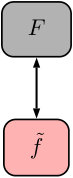 Figure 1
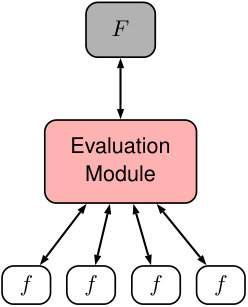 Figure 2
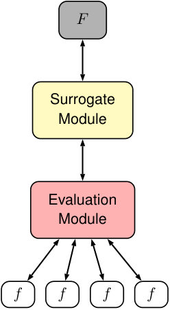 Figure 3
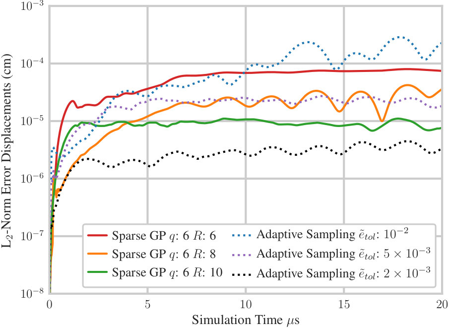 Figure 4
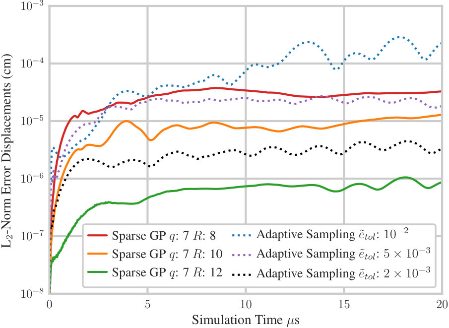 Figure 5
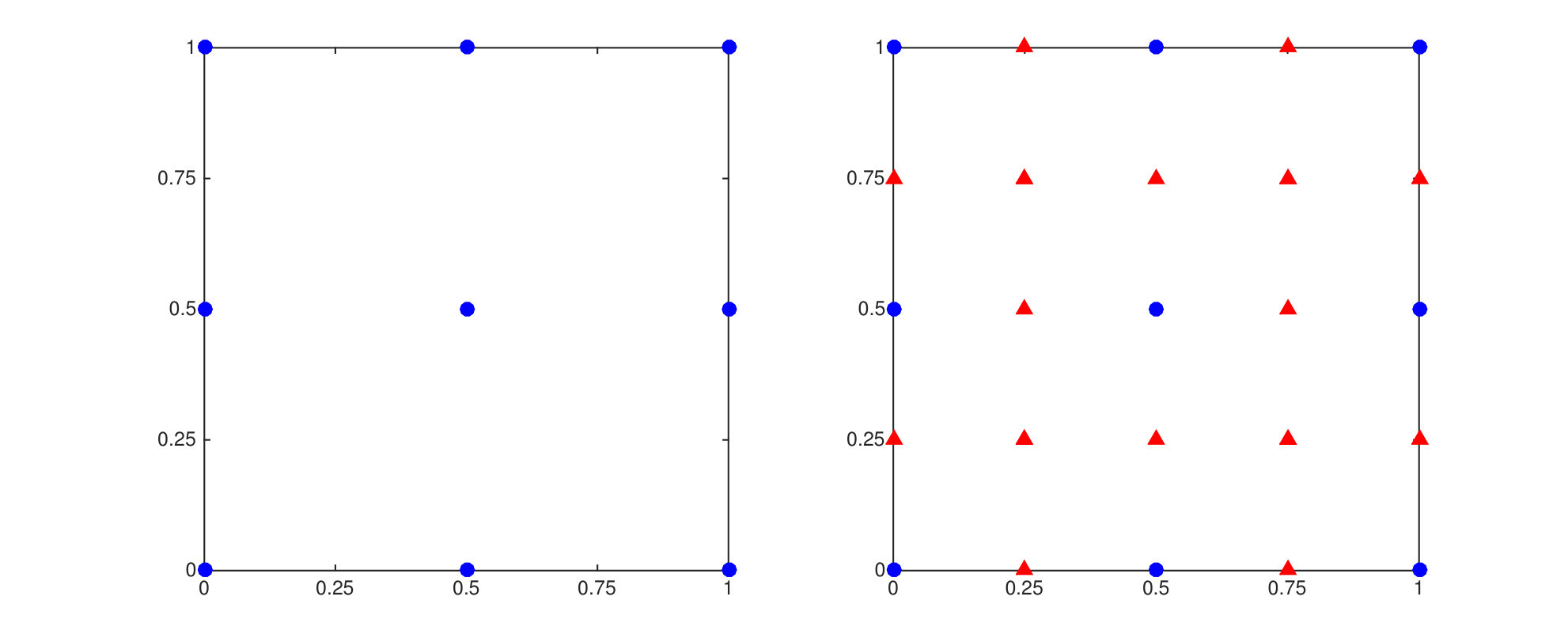 Figure 6
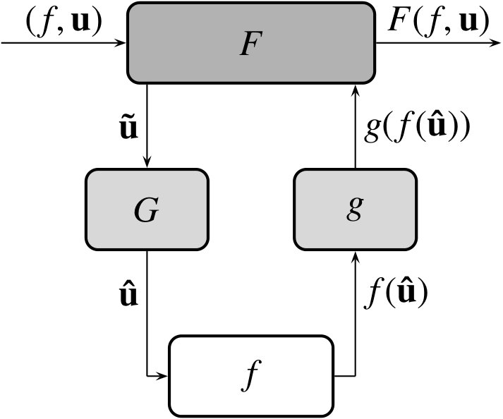 Figure 7
| Sparsity | Wall-Clock Time (hr) | Hyperparameter Opt. Time (hr) | Compute Time (hr) | # Microscale Model Evals | ||
|---|---|---|---|---|---|---|
| 6 | 6 | 0.74 | 0.9 | 0.6 | 11,504 | 4,225 |
| 6 | 8 | 0.64 | 1.5 | 0.8 | 11,525 | 4,225 |
| 6 | 10 | 0.54 | 2.7 | 1.5 | 11,561 | 4,225 |
| 7 | 8 | 0.85 | 11.4 | 8.8 | 44,345 | 16,641 |
| 7 | 10 | 0.80 | 18.4 | 15.3 | 44,570 | 16,641 |
| 7 | 12 | 0.74 | 40.9 | 32.3 | 45,274 | 16,641 |
| Wall-Clock Time (hr) | Compute Time (hr) | # Microscale Model Evals | |
|---|---|---|---|
| 2.3 | 7,546 | 833 | |
| 8.7 | 28,315 | 1,878 | |
| 156.3 | 506,333 | 27,827 | |
| No Surrogate Module | 769.2 | 9,885,192 | 2,681,600 |
Peer Reviews
No public reviews on file for this paper yet. If you reviewed it on a platform where reviews are public (OpenReview, ICLR, NeurIPS, ICML), you can paste yours below so the community can read it here.
Videos
No videos yet. Explain this paper in a talk, walkthrough, or lecture? Add one.
Accelerated scale bridging with sparsely approximated Gaussian learning
Ting Wang
Kenneth W. Leiter
Petr Plecháč
Jaroslaw Knap
Simulation Sciences Branch, RDRL-CIH-C, U.S. Army Research Laboratory
Department of Mathematical Sciences, University of Delaware
Abstract
Multiscale modeling is a systematic approach to describe the behavior of complex systems by coupling models from different scales. The approach has been demonstrated to be very effective in areas of science as diverse as materials science, climate modeling and chemistry. However, routine use of multiscale simulations is often hindered by the very high cost of individual at-scale models. Approaches aiming to alleviate that cost by means of Gaussian process regression based surrogate models have been proposed. Yet, many of these surrogate models are expensive to construct, especially when the number of data needed is large. In this article, we employ a hierarchical sparse Cholesky decomposition to develop a sparse Gaussian process regression method and apply the method to approximate the equation of state of an energetic material in a multiscale model of dynamic deformation. We demonstrate that the method provides a substantial reduction both in computational cost and solution error as compared with previous methods.
keywords:
Multiscale modeling, Gaussian regression, energetic materials, scale bridging, sparse Cholesky decomposition, gamblets
1 Introduction
Multiscale modeling has now become a de facto standard approach for the construction of high-fidelity models of complex phenomena and systems encountered in many areas of science and engineering [1, 2, 3, 4, 5, 6]. The process of building a multiscale model starts with identification of relevant phenomena occurring at individual scales, both spatial and temporal. Thereafter, appropriate at-scale models characterizing these phenomena are selected and combined together into a single multiscale model. Computation is fundamental to multiscale modeling as at-scale models are usually cast in the form of computer models. In recent years, computational aspects of multiscale modeling have become the focal point of numerous research efforts (c.f. [7] for an in-depth review of recent developments). These efforts have led to a conclusion that practicality of multiscale modeling hinges on the ability to significantly reduce the often staggering computational cost of at-scale models. Many different approaches have been proposed in order to reduce this cost, with the vast majority falling under the name of surrogate models. A surrogate model is a cheaper-to-evaluate approximation of a model, constructed from direct observations of the model. Surrogate models have been employed with great success in design optimization [8, 9], where a model is repeatedly evaluated in the search for an optimal design. In physical sciences, the use of surrogate models can be traced back to the pioneering work of Pope [10], who employed surrogate modeling to enable simulations of combustion chemistry. Other examples of the applications of surrogate models in physical sciences include crystal plasticity [11, 12], elastodynamics [13, 14], atomistic modeling [15, 16], quantum chemistry [17, 18], and fluid dynamics [19]. A comprehensive survey of surrogate modeling techniques, including polynomial regression, kriging, multivariate adaptive regression splines, polynomial stochastic collocation, adaptive stochastic collocation, and radial basis functions can be found in [20, 21].
Gaussian process regression has been advocated as a particularly flexible technique for surrogate model development [22, 23, 16]. However, due to a significant cost of construction, Gaussian process regression is rarely employed to build a single surrogate model. Instead, the domain is often partitioned into a set of subdomains and separate surrogate models are built over each of the subdomains. While such an approach inevitably reduces the overall cost of constructing a surrogate model, this reduction in cost may be accompanied by considerable disadvantages, such as, for example, the loss of smoothness of the surrogate model. In this article, we introduce a methodology to reduce the cost of constructing surrogate models based on Gaussian process regression and apply it in the context of multiscale modeling. We describe the multiscale modeling context of our work in Section 2. The details of our approach are provided in Section 3, along with an application of the technique to constructing a surrogate model of an energetic material in Section 4.
2 A computational framework for scale-bridging in multi-scale simulations
The overarching context of the developments presented in this article is the scale-bridging framework for multiscale modeling of Leiter et al. [16]. Here, we only give a brief description of the framework, the reader is referred to [16] for a full exposition. The most elemental multiscale model consists of two at-scale models, the macroscale model and the microscale model (c.f. Figure 1). The macroscale model is a mapping , where is a collection of microscale models, domain , and range . Similarly, the microscale model is a mapping where and denote the domain and range of , respectively. In addition, the framework includes two mappings to transform data between at-scale models. The mapping , where is the set of intermediate values derived from values in by . Henceforth, we refer to as the “input filter” since it generates the input to in the set . Likewise, the mapping , where , is referred to as the “output filter” as it extracts relevant data from the microscale model output to be passed to the macroscale model. More complex multiscale models can, of course, be formed through assemblies of multiple two-scale model building blocks.
The centerpiece of the scale-bridging framework is a module coordinating data exchanges between at-scale models, the Evaluation Module (c.f. Figure 2 (a)). The act of sending of from to the Evaluation Module is denoted as an evaluation request. The Evaluation Module carries out five distinct tasks: 1) it collects requests for evaluation of from ; 2) it applies the input filter to the evaluation requests to prepare input data for microscale models; 3) it schedules evaluation requests on available resources; 4) it monitors progress of evaluations to detect completion and handle failures; and 5) it applies the output filter to extract relevant data from completed evaluations to return to . However, in many practical applications, microscale models may be extremely costly to evaluate and methods to lower the evaluation cost are necessary in order to render the approach feasible. A popular approach, pioneered by Pope [10] in combustion modeling, relies on adaptive surrogate modeling, where evaluation requests are utilized to on-the-fly build an approximation to the microscale model. Such an approach is particularly advantageous as the modular structure of the scale-bridging framework allows to incorporate surrogate models with ease. Therefore, the framework can be simply augmented by the Surrogate Module operating along side of the macroscale model and the Evaluation Module (c.f. Figure 2 (b)). The role of the Surrogate Module is to automatically construct a surrogate model from completed microscale model evaluation data and subsequently employ the surrogate model in place of microscale model evaluations when appropriate. As a consequence, the use of the surrogate model in the evaluation of the microscale model is fully transparent from the viewpoint of the macroscale model.
The literature dedicated to surrogate modeling is extensive and a thorough survey of surrogate modeling approaches can be found in [20, 21]. In principle, all surrogate modeling techniques are directly applicable for construction of a surrogate model in the Surrogate Module. However, the Surrogate Model imposes two crucial constraints on the choice of surrogate model. First, an error estimate at new evaluation requests must be available so that the Surrogate Module can choose when to evaluate the surrogate model or the underlying microscale model. Second, the surrogate model must allow for the incorporation of new data acquired from the evaluation of without excessive computational cost. If the computational cost associated with updating the surrogate model is high, the use of the surrogate model may not be advantageous. A particular choice of surrogate modeling satisfying both of the above constraints and advocated by Leiter et al. is Gaussian process regression [24]. However, due to the fact that the cost of the Gaussian process regression is dominated by the inversion of the covariance matrix, a single surrogate model over the entire domain of is not constructed. Instead, a number of independent surrogate models with finite support are constructed within . It bears emphasis that the selection of training points for the construction of these surrogate models is not carried out a priori, but instead directly induced by itself. As a result, the set of all training points within is highly irregular and the set of all surrogate models does not necessarily cover in its entirety. In addition, since individual surrogate models are entirely independent, any notion of global smoothness is absent, leading to complications under the circumstances when global smoothness of approximations to is required [23]. Yet, despite of these drawbacks, the above surrogate modeling scheme is still capable of yielding remarkable savings in terms of the computational cost, enabling truly extraordinary simulations [16].
3 Accelerated surrogate model
In this section, we describe an approach to substantially reduce the cost of the construction of Gaussian surrogate models. We achieve this goal by leveraging the hierarchical sparse Cholesky decomposition recently developed by Schäfer et al. [25] in order to build an approximated global Gaussian surrogate model. Such an approach has two crucial advantages over the approach of Leiter et al. [16]. Namely, the global smoothness of approximations to is guaranteed. Additionally, construction of global surrogate models, i.e. over the entire , is feasible. Hereafter, for simplicity, we focus on a two-scale model in which the microscale model is replaced with an a priori constructed surrogate model of the microscale model (c.f. Figure. 3). We emphasize, however, that the scenario considered here will likely not always be applicable. For example, the microscale model may be composed of two or more microscale models defined over subsets of . Then, one may need to construct separate global surrogate models over each of these subsets. Alternatively, one could construct global surrogate models over some of these subsets and augment them with surrogate models of the type considered in Knap et al. [22] and Leiter et al. [16]. We do not explore these scenarios in this article, but extensions of our approach to them would be immediate. For the clarity of presentation, we restrict the input dimension of the microscale model to be . However, the described approach in this section applies to microscale models with arbitrary input dimensions.
3.1 Gaussian Process Regression
We briefly review the Gaussian process regression in this section. Suppose we have a dataset , where represents a set of inputs in a domain and represents the corresponding outputs. We aim to build a regression model to interpolate the data set and then use the interpolant to predict at a new set of locations . Gaussian process regression is a popular method for such regression problems [26]. We call a random process a Gaussian process (GP) if for any , the random vector is a -dimensional Gaussian random vector. The distribution of a GP is completely determined by its mean function and its covariance function such that
[TABLE]
and
[TABLE]
For simplicity, we assume the GP is centered, i.e., . Hence, a centered GP with covariance function can be written as
[TABLE]
We denote the covariance operator that acts on functions such that, for any suitable function (e.g., ),
[TABLE]
Often the measurement at location contains noise and hence we write
[TABLE]
where is assumed to be iid Gaussian noise that is independent with the GP . Thus, the GP model with noisy measurement turns out to be
[TABLE]
where and is the Dirac function such that if and otherwise.
Now given the data set , the Gaussian regression treats the prediction at as the mean of the conditional distribution . Since the joint distribution of is a joint Gaussian random vector
[TABLE]
it is straightforward to verity that is still a Gaussian vector with mean
[TABLE]
and covariance
[TABLE]
Finally, the mean serves as the prediction of the regression function at locations and the covariance provides a quantification of the prediction uncertainty.
As shown in the formula (3) and (4), GP regression requires the inversion of the dense covariance matrix , which is often numerically unstable. In practice, one often applies the Cholesky decomposition to such that , where is a lower triangular matrix. Nevertheless, for a dataset with observations, the computational complexity of Cholesky decomposition scales as , which becomes computationally prohibitive when . Unfortunately, this is the typical case in most multiscale problems where the construction of a high-fidelity surrogate model requires a large number of data. There exist rich literature on reducing the complexity by approximating the covariance matrix in order to accelerate the Gaussian regression for a large dataset. Most of these approximation methods can be roughly classified into two categories: (1) low rank approximation through subsampling [26] and (2) sparse approximation using inducing variables [27]. Recently, Schäfer et al. [25] proposed a novel approximated Cholesky algorithm based on the gamblet transformation [28] which reduces the bottleneck down to near linear complexity. Moreover, the upper bound of the approximation error can be shown to be exponentially small with respect to some pre-specified parameter. The algorithm, hereafter referred to as the hierarchical sparse Cholesky decomposition algorithm, requires the data points to be approximately equally spaced over the domain , which may limit its application to a general dataset. However, in the context of the multiscale bridging framework, data points from the microscale model can be sampled a priori at any location. Hence, we have the flexibility to sample data points over an uniform grid with equal spacing so that the hierarchical sparse Cholesky decomposition algorithm can be applied. In this paper, we aim to build a global Gaussian surrogate model based on the sparse Cholesky decomposition algorithm in order to accelerate the multiscale bridging.
3.2 Gamblets
The theoretical foundation of the hierarchical sparse Cholesky decomposition algorithm relies on the exponential localization property of a set of multi-resolution basis functions called gamblets [28, 29]. We briefly go over the definition of gamblets and its important properties in this section.
Given a centered Gaussian process with kernel , we define the precision/inversion operator of the covariance operator such that, for any suitable function ,
[TABLE]
The key observation is that the Gaussian process satisfies the following equation
[TABLE]
where is a centered Gaussian process with covariance operator . Also, it can be verified that the kernel is the Green’s function of (6), i.e.,
[TABLE]
Now given a data set , we define a set of basis functions called gamblets,
[TABLE]
for , i.e., it is the conditional expectation of given the observation for all and . It can be easily verified that the conditional expectation of given is a linear combination of the gamblets
[TABLE]
This is saying that the best “guess” of given the dataset is a linear combination of the observed features if all the gamblets are known. The following two properties of gamblets are crucial for deriving the hierarchical sparse Cholesky algorithm.
Representation: Each gamblet function admits the following representation in terms of the covariance kernel ,
[TABLE]
where is the inverse of the covariance matrix .
- 2.
Exponential localization: The gamblet functions are exponentially decaying in the sense that
[TABLE]
for some constants , where is the - inner product and is some distance between and . This property provides the theoretical foundation to sparsely approximate the dense covariance matrix.
3.3 Multi-resolution gamblets and block Cholesky decomposition
In this section, we provide a heuristic derivation for the hierarchical sparse Cholesky decomposition. The algorithm assumes that the configuration of the input set are nested with levels. For ease of presentation, throughout of this section we set so that the two-level input set forms an uniform grid of resolution over the domain . The two-level input set can be obtained by subdividing the level-one grid , where is the set of input points that forms the uniform grid with resolution (c.f. Figure 4). Similarly, the -level uniform grid with resolution can be obtained by recursively subdividing for times. We denote and the index sets of points in and respectively. That is, whenever for . We henceforth write to emphasize the fact that is a point in . Clearly, is a subset of and hence we can define the index set and , i.e., contains the index of those data points that are in but not in . Hence, we can classify the points in into two categories: contains level two points that are also in level one and contains points that are in level two but not in level one.
The above recursive sampling procedure can be viewed as a two-step hierarchical sampling approach, where a fine dataset is sampled on top of the coarse dataset . Now given the datasets and , we denote by
[TABLE]
and
[TABLE]
their corresponding covariance matrices. Following the definition of gamblets in (7), we can define the level one and level two gamblets by
[TABLE]
and
[TABLE]
respectively. Using the definition of operator and the representation (8), it can be readily shown that the following two matrices
[TABLE]
and
[TABLE]
are the inverse of the covariance matrices and respectively. Hence, hereafter we refer as the precision matrix associated with the dataset for . It is immediate that each precision matrix is exponentially localized (i.e., nearly sparse) due to the exponential localization of gamblets. Let us write the precision matrix in a block matrix form (corresponding to sets and )
[TABLE]
To be consistent, we also write the level one precision matrix as a single block matrix
[TABLE]
Owhadi and Scovel [28, 30] have proved that for a wide range of kernel functions , the conditional numbers of the block matrices and are bounded. Based on this fact, they have further shown that the inverses matrices and are exponentially localized as well.
With the above preparations, now we are ready to motivate the hierarchical sparse Cholesky decomposition algorithm. We start by making an important observation that links block Cholesky decomposition (or decomposition) with the two level hierarchical sampling procedure that we illustrated above. Recall that is the covariance matrix associated with the two-level dataset . Its block Cholesky decomposition (corresponding to and ) reads
[TABLE]
where is the covariance matrix between and . Since is the inverse of the precision matrix , basic linear algebra shows that
[TABLE]
and the Schur complement
[TABLE]
Hence the block Cholesky decomposition of can be rewritten in terms of as
[TABLE]
where and are the Cholesky factors of and respectively, i.e.,
[TABLE]
and
[TABLE]
An application of Cauchy-Schwarz inequality to (11) shows that the off-diagonal part of the Cholesky factor is exponentially localized. Furthermore, the result (Theorem ) in [25] shows that the block Cholesky factors and are also exponentially localized. This suggests that the entire Cholesky factor in (13) is exponentially localized. In other words, up to exponentially small entries, the Cholesky factor of is nearly sparse and the sparsity pattern is known a priori. Therefore, it is desirable to skip the exponentially small entries in the process of Cholesky factorization in order to reduce the computational complexity, which leads to the basic idea of the hierarchical sparse Cholesky decomposition.
3.4 The sparse GP algorithm
The above heuristic derivation is based on a dataset over a two-level uniform grid. However, the same argument can be easily extended for a dataset over a level uniform grid by successively doing the block Cholesky decomposition (13) for times, which leads to the block Cholesky decomposition
[TABLE]
Since the locations (row and column) of those exponentially small entries in are explicitly known, with a certain confidence level, we can sparsely approximate by replacing these entries by zero. Schäfer et al. [25] define the set of sparsity pattern to be
[TABLE]
where is a parameter that controls the level of sparsity. Then they suggest to restrict the Cholesky computation only to this sparsity set through applying the zero fill-in incomplete Cholesky decomposition [31] to the sparse matrix
[TABLE]
such that . Here the incomplete Cholesky factor is obtained by stepping through the Cholesky reduction on setting to zero if the corresponding is zero. Finally, the main result in [25] asserts that we can use to approximate the original dense covariance matrix such that
[TABLE]
for some constant and polynomial , where the constant is independent of . Moreover, the computational complexity for obtaining is , which is near linear in . Hence, the sparsity parameter controls the trade-off between efficiency and accuracy. With larger , the error bound is decreased but the complexity is increased. Finally, the sparse GP algorithm that uses the hierarchical sparse Cholesky decomposition for Gaussian regression is as follows.
A few comments are in order: Note that the above algorithm is simply the standard Gaussian regression with the Cholesky decomposition of replaced by the incomplete Cholesky of its sparse approximation . Hence, the algorithm can be easily implemented on top of the standard GP algorithm. It is important that the input points in the dataset are order from to for the algorithm to work correctly. In the case that the data are not sample in this order, we can identity a permutation matrix such that has the correct ordering. Our presentation of Algorithm 1 assumes that the configuration of the input set is strictly uniform over the domain . However, we point out that this is requirement can be relaxed. Indeed, the algorithm is robust as long as the input configuration satisfies some certain criteria (c.f. [25] for more details).
4 Results
We now assess the sparse GP method in the context of a computationally demanding multiscale model of impact physics. The multiscale model consists of two at-scale models, a continuum mechanics macroscale model and a particle-based microscale model. The surrogate model serves to replace evaluation of the microscale model at a significantly reduced computational cost. The new sparse GP method is compared with the adaptive sampling based approach of Leiter et al. [16], summarized below, which constructs individual surrogate models on subsets of the entire training dataset.
4.1 Macroscale model
The macroscale model is a continuum mechanics model of a deforming body implemented in the ALE3D multi-physics finite-element code [32]. The material of the body is taken to be the energetic 1,3,5-trinitrohexahydro-s-triazine (RDX) and its equation of state (EOS) is obtained through evaluation of the microscale model. The EOS provides the pressure, , and temperature, , for a given mass density, , and internal energy density, . The macroscale model uses a modified predictor-corrector algorithm to integrate energy forward in time. The predictor step includes the pressure volume work over the first half of the timestep plus strain work from the deviatoric stress: , where is the energy density at the start of the timestep, is the pressure at the start of the timestep, is the change in relative volume over the timestep, and is the change in deviatoric strain energy density. The deviatoric strain energy is computed using a conventional -plasticity model with Steinberg-Guinan hardening [33] with a yield strength of 150 MPa, hardening coefficient of 200 and hardening exponent of 0.1. The predictor pressure and temperature are computed using the EOS as
[TABLE]
where is the mass density at the end of the timestep. The corrector step updates the energy as giving the pressure and temperature at the end of the step as
[TABLE]
At modest pressures, the energy update in the corrector step is small, which leads to a small change in pressure. In order to avoid a second EOS evaluation per timestep, the pressure and temperature corrections are omitted in our approach. The energy is updated, but the temperature and pressure updates lag behind:
[TABLE]
4.2 Microscale model
The microscale model computes the EOS using energy-conserving dissipative particle dynamics (DPD). The simulations are managed by the LAMMPS Integrated Materials Engine (LIME), a Python wrapper to LAMMPS that automates EOS evaluation [34]. LIME initializes and equilibrates a simulation cell containing 21,952 particles (28 x 28 x 14 unit cells) of RDX to be consistent with the prescribed mass density and energy density. Following equilibration, the temperature and pressure of the system are computed via ensemble averages.
4.3 Adaptive sampling
The adaptive sampling method reduces computational cost of expensive multiscale models. We refer the reader to Knap et al. [22] and Leiter et al. [16] for a detailed description of the adaptive sampling algorithm and its implementation in the scale-bridging framework, but will briefly describe the method here. Adaptive sampling is an active learning algorithm that constructs a set of local GP surrogate models on-the-fly to replace the evaluation of computationally expensive microscale models. In the case of the multiscale model considered here, the surrogate models approximate the EOS computed using DPD. While the macroscale model integrates its solution forward in time, it repeatedly evaluates the EOS. With adaptive sampling, the EOS is either evaluated by a surrogate model or by the microscale model. An error estimate of the surrogate model for a particular and is compared to a user-specified acceptable error tolerance parameter, , to determine if the EOS evaluation is satisfied by the surrogate model. If the error estimate is too high, the EOS is computed by the microscale model and the result is used to update the surrogate model. The adaptive sampling algorithm continuously improves the accuracy of the surrogate model for regions of the EOS of interest to the macroscale model. The number of data to be incorporated into a surrogate model may be potentially very large, especially for low values of . The computational cost of GP regression scales as where is the number of data. Rather than construct a single GP surrogate model across all of the data, the adaptive sampling algorithm builds a number of local GP surrogate models on a partition of the overall data. A parameter determines the maximum number of data per local surrogate model. The collection of surrogate models is stored in a metric-tree database to allow quick access for evaluation and update.
Although adaptive sampling has been very successful in reducing computational cost of expensive multiscale models [22, 11, 16] it suffers two significant drawbacks in practice: 1) the patchwork collection of local GP surrogate models gives no guarantee of continuity between the patches; 2) the overall simulation is often highly load imbalanced due to the unpredictable adaptive execution of expensive microscale models.
4.4 Taylor impact simulation
We compare the performance of the sparse GP method and the adaptive sampling method for the simulation of a Taylor impact experiment, commonly used to characterize the deformation behavior of materials [35]. The simulation setup is identical to the one in [16]. In a Taylor impact experiment, a cylinder of material travels at a constant initial velocity and impacts a rigid anvil. In the simulations presented here, the cylinder of RDX has a height of 1.27 cm and radius of 0.476 cm and travels at 200 m/s. In the macroscale model, axisymmetry is imposed along the cylinder axis and the cylinder is decomposed into 1600 first-order quadrilateral elements. We simulate the impact for 20 s using an adaptive timestep with the initial timestep set to 0.001 s and the maximum allowable timestep set to 0.012 s for a total of 1,676 timesteps. The simulations are executed on the SGI ICE X high performance computer ”Topaz” at the Engineering Research and Development Center.
For simulations that use the sparse GP method, only a single compute node, containing a 36 core 2.3 GHz Intel Xeon Haswell processor, is used because all of the microscale model data is precomputed. The microscale model is computed for values of between J/m3 and J/m3 and for between 1.75 g/cm3 and 1.93 g/cm3. The bounds are selected based upon previous experience running the simulation. The requirement to select appropriate bounds for the grid sampling is a drawback of the sparse GP method compared to the adaptive sampling method, which is able to expand the sampling region during model evaluation on-demand. Two sets of microscale model data are obtained corresponding to and , for a total of 4,225 and 16,641 points respectively. For each level , three Taylor impact simulations are performed under different values of the sparsity parameter : = 6, 8, and 10 for and = 8, 10, and 12 for . The squared exponential kernel
[TABLE]
is used for the GP, where the hyperparameter is the length-scale, is the signal variance and is the noise variance. The choice of the squared exponential kernel reflects our prior belief that the microscale model outputs are smooth and hence we seek a smooth approximation. Hyperparameters for the sparse GP surrogate model are obtained by minimizing the negative log marginal likelihood (NLML) with the BFGS algorithm implemented in the dlib C++ toolkit [36] using a stopping criterion of . The starting point for the hyperparameter optimization is chosen to be , , and .
Simulations employing the adaptive sampling method are executed on a total of 90 compute nodes for a total of 3,240 cores. The macroscale model and adaptive sampling module are executed on a single node, with the remaining 89 compute nodes dedicated to microscale model evaluations. The maximum number of points per local surrogate model, is chosen to be . Three simulations are performed under different : , , and .
The results of the adaptive sampling and sparse GP simulations are compared to those of a reference simulation computing the microscale DPD model for all EOS evaluations of the macroscale model. The reference simulation requires a total of 2,681,600 microscale model evaluations and completes in 32.05 days of wall-clock time on 12,852 processor cores for a total compute time of 9,885,192 hours.
4.5 Results
Timing data for Taylor impact simulations with the sparse GP surrogate model are presented in Table 1. Here the sparsity is the fraction of non-zeros in the covariance matrix that are replaced by zeros in the sparse covariance matrix (c.f. (14)). The compute time includes the time required to evaluate the microscale model for input points of grid level , the time to optimize the hyperparameters of the model, and the time to execute the Taylor impact simulation. The compute time to sample the microscale model at grid points is 11,475 hr for and 43,980 hr for . This indicates that for all simulations with the sparse GP surrogate model, the vast majority of total compute time, greater than 95%, is spent sampling the microscale model. We note, however, that sampling the microscale model incurs a one-time expense for a particular and the data can be reused across multiple simulations. In addition, the sampling points are nested across levels, which allows some microscale model data to be reused from lower levels. Obtaining microscale model results at sampling points is embarrassingly parallel as all points are chosen ahead of time for a particular value of . Given sufficient computing resources, the microscale model data can be obtained in a very short amount of wall-clock time. Therefore, the wall-clock time given in Table 1 omits time spent precomputing the microscale model and includes only the time to optimize hyperparameters, dependent on the choice of , and the time required to complete the Taylor impact simulation. A significant portion of the wall-clock time, ranging from 50% to 83% is spent on optimization of the hyperparameters. The remaining time is spent on evaluation of the surrogate model and the integration of the macroscale model forward in time.
For comparison, we present timing data in Table 2 for simulations that use adaptive sampling. A detailed discussion of these timings can be found in [16]. It should be noted here that both the adaptive sampling method and the sparse GP method allow for simulations that are orders of magnitude cheaper than the benchmark simulation which always obtains the EOS from the microscale model.
We now assess the effect of grid level and sparsity parameter on the solution of the Taylor impact problem. In Figure 5, we plot the -norm of the error in the displacements predicted by the macroscale model as a function of simulation time for sparse GP simulations with . For comparison, we also plot the error for the adaptive sampling simulations with of , and . The -norm of the error in the displacements field is:
[TABLE]
where is the -th component of the the displacements field obtained from the simulation employing a surrogate model, is the -th component of the field from the reference simulation, and denotes the volume of the cylinder.
As is increased, the error in displacements is reduced. The sparse GP simulation with and has an error roughly equivalent to the adaptive sampling simulation with , but uses only 17% of the wall-clock time and 41% the compute time. The simulation with and has a lower error than the adaptive sampling simulation with , but requires only 31% of the wall-clock time and of the compute time. These results demonstrate that the sparse GP method provides a more accurate solution than the adaptive sampling method at a fraction of the wall-clock and simulation time.
For , the number of microscale model evaluations is 4,225, which is more than twice as many as used in the adaptive sampling simulation with . It may appear surprising that the cost of the sparse GP simulations, in terms of both wall-clock time and compute time, are less than those using adaptive sampling despite the many more microscale model evaluations used. However, the reduction in cost is completely a consequence of the computational load imbalance inherent in the adaptive sampling method that is not present when using the sparse GP surrogate model. In adaptive sampling, many processors are left underutilized during long stretches of the simulation due to the unpredictable on-demand evaluation of microscale models, a major drawback to the method. In the sparse GP approach, all microscale model data is precomputed ahead of time and is perfectly scalable and computationally efficient. Computational resources are also fully utilized throughout the simulation itself, spent primarily on the evaluation of the EOS using the surrogate model.
None of the sparse GP simulations with reduce the error below that obtained using adaptive sampling with the lowest . Further simulations with and values of beyond , not included here, provide no further reduction in the error. To determine whether the error of sparse GP simulations can be reduced further by increasing the amount of microscale model data available, the error in the displacements field for sparse GP simulations with is plotted in Figure 6. In fact, the error is reduced further by using a higher . As was the case with , increasing reduces the error in the solution. The sparse GP simulation with and provides an error in displacements well below the smallest error obtained using adaptive sampling with and is able to achieve the reduced error with 26% of the wall-clock time and 9% of the compute time, a significant improvement. Furthermore, the sparse GP surrogate model uses many fewer microscale model evaluations, only 16,641, compared to the 27,827 microscale model evaluations required by the most accurate adaptive sampling simulation. This is especially strong evidence of the advantage of the sparse GP method. Given even fewer samples of the microscale model, the sparse GP method produces a more accurate surrogate model than adaptive sampling.
One interesting comparison can also be made between two of the sparse GP simulations, one with parameters and and another with and . Both simulations have roughly the same error in the solution, despite the increase in microscale model data available for the simulation run. This observation can be explained by the error bound (15). For sparse GP with , the polynomial term in the error bound may be significantly larger than that of the sparse GP with , which offsets the higher accuracy provided by the finer sampling. This indicates that when less accuracy is required, a good strategy may be to avoid over sampling the microscale model as a coarse sampling should be sufficient.
5 Summary
In this article, we have described a formulation of a sparse GP regression method based on the near linear complexity sparse Cholesky algorithm of Schäfer et al. [25]. The sparse GP method is capable of utilizing a large number of training data and, thus, avoiding a bottleneck associated traditionally with GP methods. This behavior is due to the fact that the dense covariance matrix admits an approximate sparse Cholesky decomposition, which reduces the computational complexity down to near linear in . In addition, the sparse GP method provides error bounds for the sparse approximation that are exponentially small with respect to a chosen sparsity parameter.
Subsequently, we have employed the sparse GP method to construct a surrogate model for a microscale model in a two-scale model of deformation of an energetic material. The microscale model characterizes the volumetric response of the energetic material by recourse to dissipative particle dynamics. In turn, the macroscopic model is a finite-element model simulating dynamic deformation. We have considered two scenarios: 1) the evaluation of the microscale model is replaced by an adaptive sampling approach, amounting to on-the-fly construction of GP surrogates with compact support; 2) the evaluation of the microscale model is replaced by a sparse GP surrogate model constructed over the entire domain of the microscale model. We have contrasted these two scenarios in terms of the overall computational cost required to construct the surrogate models and perform simulations with the macroscopic model.
Our results indicate that the sparse GP surrogate model offers remarkable computational savings over the adaptive sampling surrogate model. In some cases, these savings translate into over 10-fold reduction in terms of the computational cost. This reduction is primarily due to the fact that the sparse GP surrogate model relies on a fixed grid for the selection of sampling points and the sampling can be easily carried out with an extraordinary level of concurrency. Of course, appropriate bounds for the extents of the grid must be selected a priori as to guarantee that all evaluations requested by the macroscopic model will ultimately be fully contained within the grid. We emphasize that the adaptive sampling surrogate model does not suffer from such a limitation as it is constructed adaptively and can incorporate data from any subset of the domain. However, in practice, good estimates for the bounds may be easily available from, for example, lower fidelity microscale models.
In addition to the computational savings offered by the sparse GP method, it also leads to a greater accuracy in the displacement field than the local GP models constructed in the adaptive sampling method. The increase in accuracy of the sparse GP method is likely because it takes into account the long range correlations between data points, which are not included when the data is partitioned into separate GP surrogates with compact support.
It should be pointed out that the EOS regression problem showcased here is low dimensional and that additional methods will be required to extend GP regression to high dimensions, such as active subspaces [37] or additive kernels [38]. Sparse GP regression helps to alleviate the problem of high dimensionality somewhat by enabling the incorporation of more data into the surrogate model. Perhaps combining dimension reduction methods with the sparse GP method outlined here could address even higher dimensional problems and is a subject of ongoing research.
6 Acknowledgements
The authors would like to thank Dr. Rich Becker of the U.S. Army Research Laboratory and Florian Schäfer of Caltech for fruitful discussions. The work of T.W. and P.P. was supported in part by the DARPA project W911NF-15-2-0122. This work was supported in part by a grant of computer time from the DoD High Performance Computing Modernization Program at the U.S. Army Engineer Research and Development Center.
References
- [1]
W. A. Curtin, R. E. Miller, Atomistic/continuum coupling in computational materials science, Modelling and Simulation in Materials Science and Engineering 11 (3) (2003) R33.
- [2]
F. Pelupessy, A. van Elteren, N. de Vries, S. McMillan, N. Drost, S. P. Zwart, The astrophysical multipurpose software environment, Astronomy & Astrophysics 557 (2013) A84.
- [3]
V. S. Mahadevan, E. Merzari, T. Tautges, R. Jain, A. Obabko, M. Smith, P. Fischer, High-resolution coupled physics solvers for analysing fine-scale nuclear reactor design problems, Philosophical Transactions of the Royal Society of London A: Mathematical, Physical and Engineering Sciences 372 (2021).
- [4]
J. L. Suter, D. Groen, P. V. Coveney, Chemically specific multiscale modeling of clay-polymer nanocomposites reveals intercalation dynamics, tactoid self-assembly and emergent materials properties, Advanced Materials 27 (6) (2015) 966–984.
- [5]
P. Perdikaris, L. Grinberg, G. E. Karniadakis, Multiscale modeling and simulation of brain blood flow, Physics of Fluids 28 (2) (2016) 021304.
- [6]
S. Alowayyed, D. Groen, P. V. Coveney, A. G. Hoekstra, Multiscale computing in the exascale era, Journal of Computational Science 22 (2017) 15 – 25.
- [7]
D. Groen, J. Knap, P. Neumann, D. Suleimenova, L. Veen, K. Leiter, Mastering the scales: a survey on the benefits of multiscale computing software, Philosophical Transactions A, (in print).
- [8]
G. G. Wang, S. Shan, Review of metamodeling techniques in support of engineering design optimization, Journal of Mechanical Design 129 (4) (2007) 370–380.
- [9]
S. Koziel, D. E. Ciaurri, L. Leifsson, Surrogate-based methods, in: Computational Optimization, Methods and Algorithms, Springer Berlin Heidelberg, 2011, Ch. 3, pp. 33–59.
- [10]
S. Pope, Computationally efficient implementation of combustion chemistry using in situ adaptive tabulation, Combustion Theory and Modelling 1 (1) (1997) 41–63.
- [11]
N. R. Barton, J. Knap, A. Arsenlis, R. Becker, R. D. Hornung, D. R. Jefferson, Embedded polycrystal plasticity and adaptive sampling, International Journal of Plasticity 24 (2) (2008) 242–266.
- [12]
H. F. Alharbi, S. R. Kalidindi, Crystal plasticity finite element simulations using a database of discrete fourier transforms, International Journal of Plasticity 66 (2015) 71 – 84.
- [13]
B. Rouet-Leduc, K. Barros, E. Cieren, V. Elango, C. Junghans, T. Lookman, J. Mohd-Yusof, R. S. Pavel, A. Y. Rivera, D. Roehm, A. L. McPherson, T. C. Germann, Spatial adaptive sampling in multiscale simulation, Computer Physics Communications 185 (7) (2014) 1857 – 1864.
- [14]
D. Roehm, R. S. Pavel, K. Barros, B. Rouet-Leduc, A. L. McPherson, T. C. Germann, C. Junghans, Distributed database kriging for adaptive sampling (D2KAS), Computer Physics Communications 192 (2015) 138–147.
- [15]
Z. Li, J. R. Kermode, A. De Vita, Molecular dynamics with on-the-fly machine learning of quantum-mechanical forces, Physical Review Letters 114 (2015) 096405.
- [16]
K. W. Leiter, B. C. Barnes, R. Becker, J. Knap, Accelerated scale-bridging through adaptive surrogate model evaluation, Journal of Computational Science 27 (2018) 91–106.
- [17]
M. Rupp, A. Tkatchenko, K.-R. Müller, O. A. von Lilienfeld, Fast and accurate modeling of molecular atomization energies with machine learning, Phys. Rev. Lett. 108 (2012) 058301.
- [18]
R. Gómez-Bombarelli, J. N. Wei, D. Duvenaud, J. M. Hernández-Lobato, B. Sánchez-Lengeling, D. Sheberla, J. Aguilera-Iparraguirre, T. D. Hirzel, R. P. Adams, A. Aspuru-Guzik, Automatic chemical design using a data-driven continuous representation of molecules, ACS Central Science 4 (2) (2018) 268–276.
- [19]
L. Zhao, Z. Li, B. Caswell, J. Ouyang, G. E. Karniadakis, Active learning of constitutive relation from mesoscopic dynamics for macroscopic modeling of non-newtonian flows, Journal of Computational Physics 363 (2018) 116 – 127.
- [20]
R. Jin, W. Chen, T. Simpson, Comparative studies of metamodelling techniques under multiple modelling criteria, Structural and Multidisciplinary Optimization 23 (1) (2001) 1–13.
- [21]
O. Sen, S. Davis, G. Jacobs, H. Udaykumar, Evaluation of convergence behavior of metamodeling techniques for bridg ing scales in multi-scale multimaterial simulation, Journal of Computational Physics 294 (2015) 585–604.
- [22]
J. Knap, N. R. Barton, R. D. Hornung, A. Arsenlis, R. Becker, D. R. Jefferson, Adaptive sampling in hierarchical simulation, International Journal for Numerical Methods in Engineering 76 (4) (2008) 572–600.
- [23]
N. R. Barton, J. V. Bernier, J. Knap, A. J. Sunwoo, E. K. Cerreta, T. J. Turner, A call to arms for task parallelism in multi-scale materials modeling, International Journal for Numerical Methods in Engineering 86 (6) (2011) 744–764.
- [24]
C. E. Rasmussen, C. K. I. Williams, Gaussian Processes for Machine Learning (Adaptive Computation and Machine Learning), MIT Press, 2005.
- [25]
F. Schäfer, T. J. Sullivan, H. Owhadi, Compression, inversion, and approximate pca of dense kernel matrices at near-linear computational complexity, arXiv preprint arXiv:1706.02205.
- [26]
C. E. Rasmussen, Gaussian processes in machine learning, in: Advanced lectures on machine learning, Springer, 2004, pp. 63–71.
- [27]
J. Quiñonero-Candela, C. E. Rasmussen, A unifying view of sparse approximate gaussian process regression, Journal of Machine Learning Research 6 (Dec) (2005) 1939–1959.
- [28]
H. Owhadi, Multigrid with rough coefficients and multiresolution operator decomposition from hierarchical information games, SIAM Review 59 (1) (2017) 99–149.
- [29]
H. Owhadi, Bayesian numerical homogenization, Multiscale Modeling & Simulation 13 (3) (2015) 812–828.
- [30]
H. Owhadi, C. Scovel, Universal scalable robust solvers from computational information games and fast eigenspace adapted multiresolution analysis, arXiv preprint arXiv:1703.10761.
- [31]
G. H. Golub, C. F. Van Loan, Matrix computations, Vol. 3, JHU Press, 2012.
- [32]
A. Anderson, R. Cooper, R. Neely, A. Nichols, R. Sharp, B. Wallin, Users manual for ALE3D–an arbitrary Lagrange/Eulerian 3D code system, LLNL, Version 3 (1).
- [33]
D. J. Steinberg, S. G. Cochran, M. W. Guinan, A constitutive model for metals applicable at high-strain rate, Journal of Applied Physics 51 (3) (1980) 1498–1504.
- [34]
B. C. Barnes, K. W. Leiter, R. Becker, J. Knap, J. K. Brennan, LAMMPS integrated materials engine (LIME) for efficient automation of particle-based simulations: application to equation of state generation, Modelling and Simulation in Materials Science and Engineering 25 (5) (2017) 055006.
- [35]
G. Taylor, The use of flat-ended projectiles for determining dynamic yield stress. I. Theoretical considerations, Proceedings of the Royal Society of London A: Mathematical, Physical and Engineering Sciences 194 (1038) (1948) 289–299.
- [36]
D. E. King, Dlib-ml: A machine learning toolkit, Journal of Machine Learning Research 10 (2009) 1755–1758.
- [37]
R. Tripathy, I. Bilionis, M. Gonzalez, Gaussian processes with built-in dimensionality reduction: Applications to high-dimensional uncertainty propagation, Journal of Computational Physics 321 (2016) 191 – 223.
- [38]
D. K. Duvenaud, H. Nickisch, C. E. Rasmussen, Additive gaussian processes, Advances in Neural Information Processing Systems 24 (2011) 226–234.
The reference list from the paper itself. Each links out to its DOI / PubMed record.
- 1[1] W. A. Curtin, R. E. Miller, Atomistic/continuum coupling in computational materials science, Modelling and Simulation in Materials Science and Engineering 11 (3) (2003) R 33.
- 2[2] F. Pelupessy, A. van Elteren, N. de Vries, S. Mc Millan, N. Drost, S. P. Zwart, The astrophysical multipurpose software environment, Astronomy & Astrophysics 557 (2013) A 84.
- 3[3] V. S. Mahadevan, E. Merzari, T. Tautges, R. Jain, A. Obabko, M. Smith, P. Fischer, High-resolution coupled physics solvers for analysing fine-scale nuclear reactor design problems, Philosophical Transactions of the Royal Society of London A: Mathematical, Physical and Engineering Sciences 372 (2021).
- 4[4] J. L. Suter, D. Groen, P. V. Coveney, Chemically specific multiscale modeling of clay-polymer nanocomposites reveals intercalation dynamics, tactoid self-assembly and emergent materials properties, Advanced Materials 27 (6) (2015) 966–984.
- 5[5] P. Perdikaris, L. Grinberg, G. E. Karniadakis, Multiscale modeling and simulation of brain blood flow, Physics of Fluids 28 (2) (2016) 021304.
- 6[6] S. Alowayyed, D. Groen, P. V. Coveney, A. G. Hoekstra, Multiscale computing in the exascale era, Journal of Computational Science 22 (2017) 15 – 25.
- 7[7] D. Groen, J. Knap, P. Neumann, D. Suleimenova, L. Veen, K. Leiter, Mastering the scales: a survey on the benefits of multiscale computing software, Philosophical Transactions A, (in print).
- 8[8] G. G. Wang, S. Shan, Review of metamodeling techniques in support of engineering design optimization, Journal of Mechanical Design 129 (4) (2007) 370–380.