Polynomial invariants for links and tied links
Jes\'us Juyumaya

TL;DR
This paper discusses polynomial invariants used to distinguish links and tied links, based on lessons from specialized courses and conferences, highlighting their theoretical foundations and applications.
Contribution
It introduces or analyzes polynomial invariants specifically for links and tied links, expanding the understanding of their algebraic and topological properties.
Findings
Development of new polynomial invariants for tied links
Application of invariants to classify complex link structures
Insights into algebraic relations among invariants
Abstract
Notes based on lessons given at {\sc Escuela " Fico Gonz\'alez Acu\~na" de Nudos y 3-variedades}, M\'erida Yucat\'an, M\'exico, 7--10 (2015) and {\sc Encuentro de nudos, trenzas y \'algebras}, Oaxaca--M\'exico, 3--10 October (2018).
Click any figure to enlarge with its caption.
 Figure 1
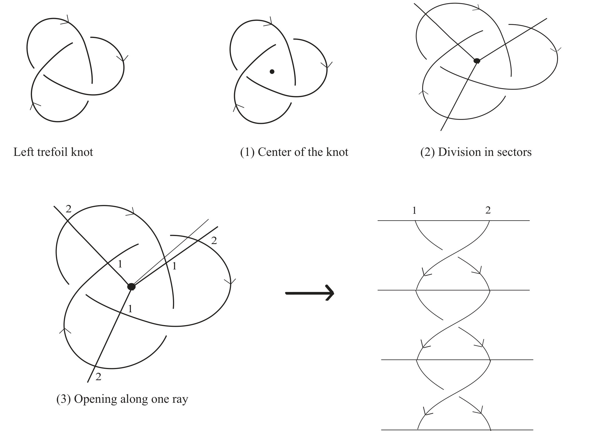 Figure 2
 Figure 3
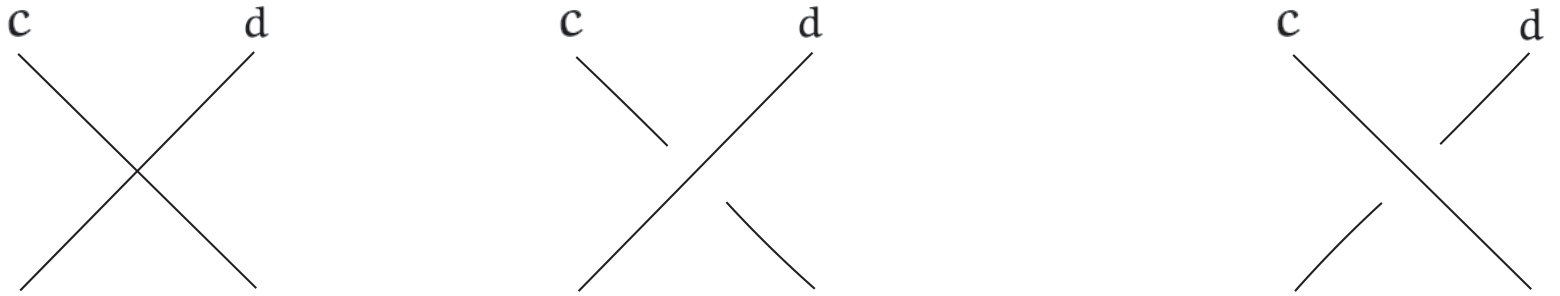 Figure 4
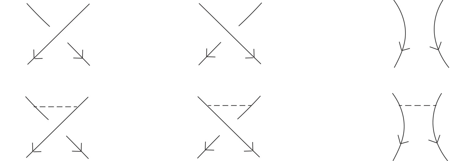 Figure 5
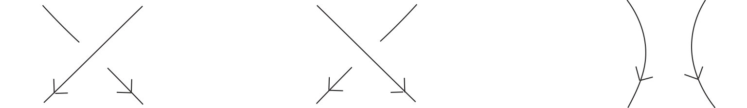 Figure 6
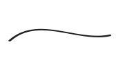 Figure 7
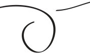 Figure 8
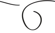 Figure 9
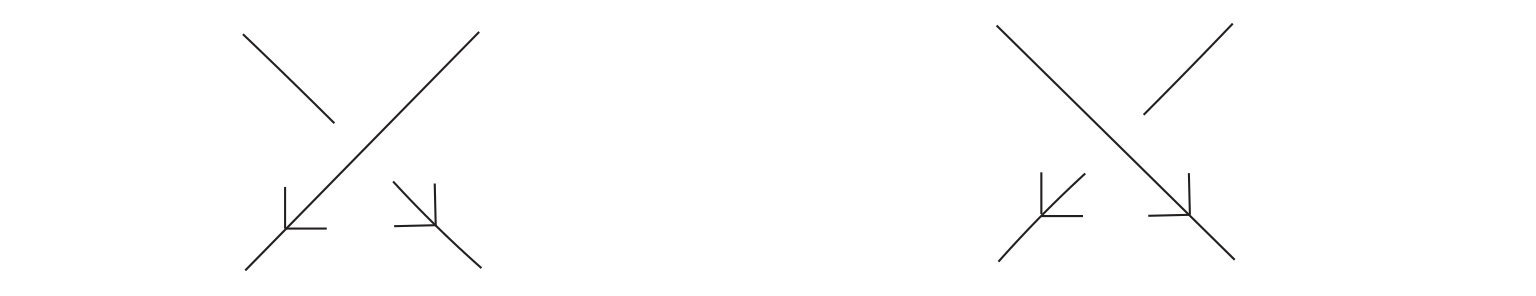 Figure 10
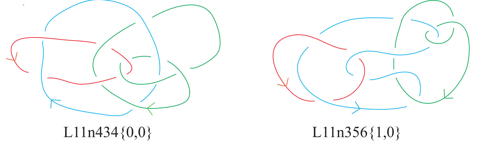 Figure 11
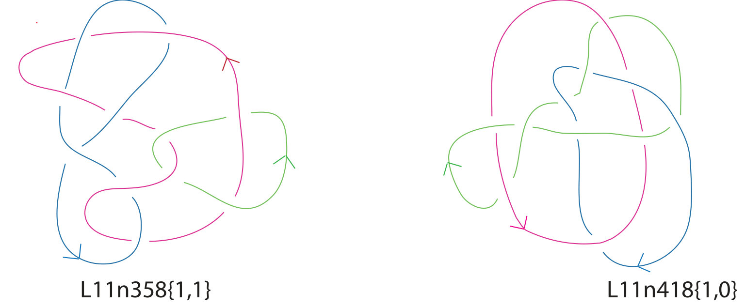 Figure 12
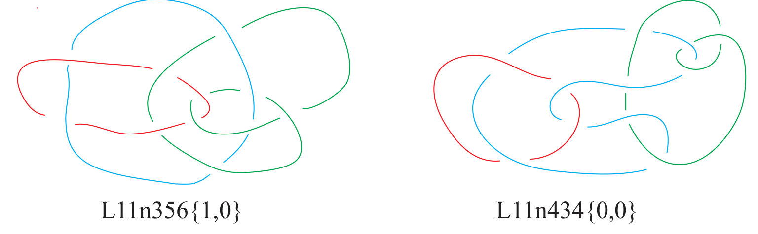 Figure 13
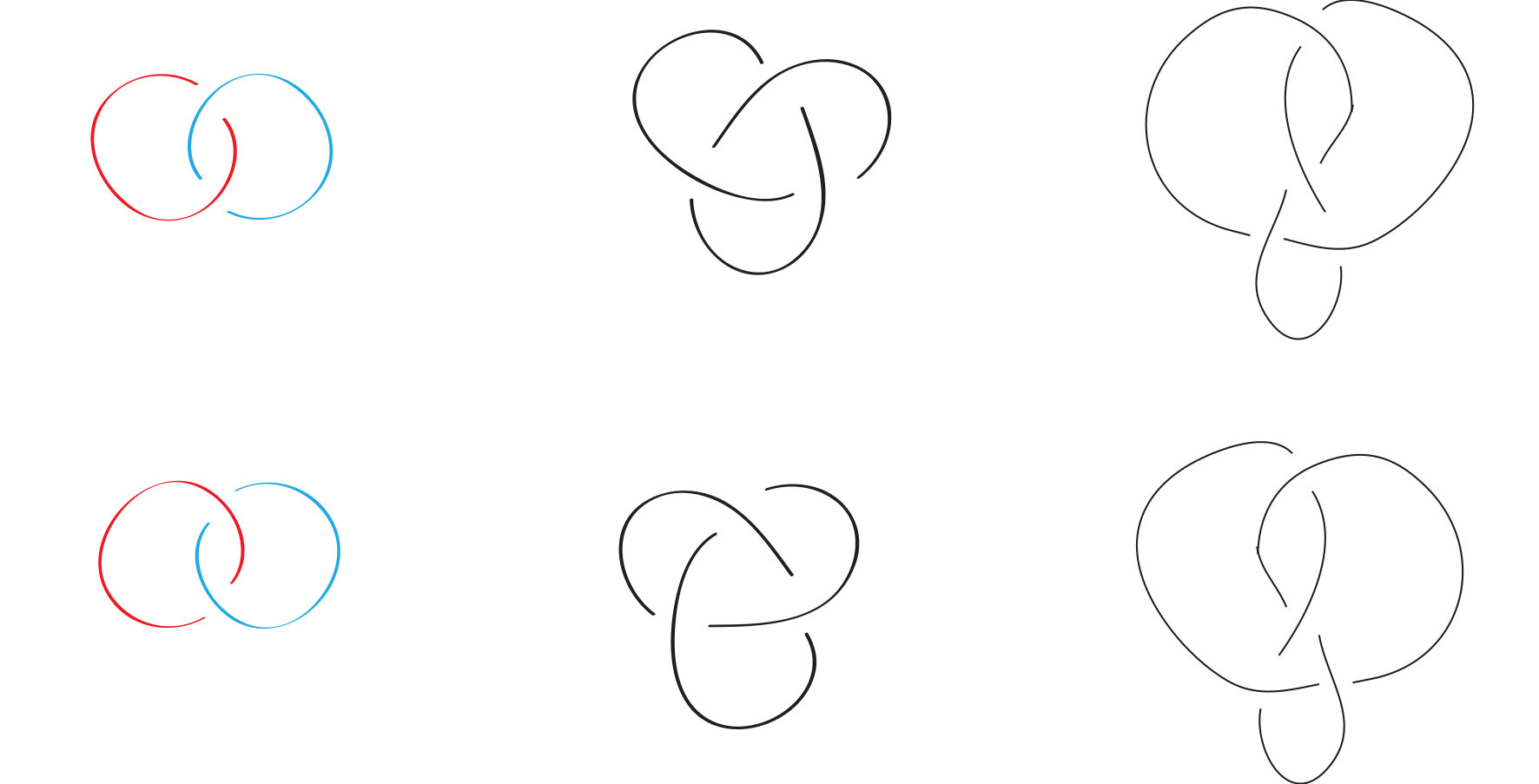 Figure 14
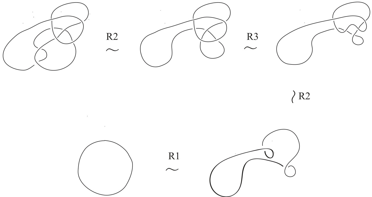 Figure 15
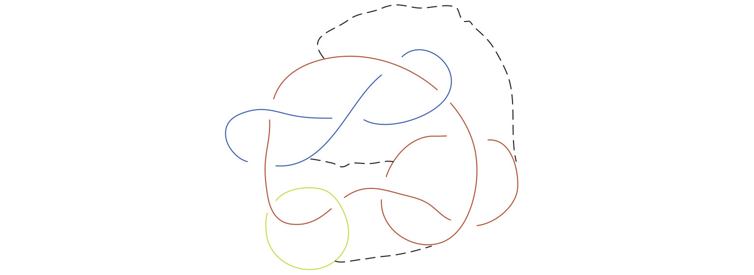 Figure 16
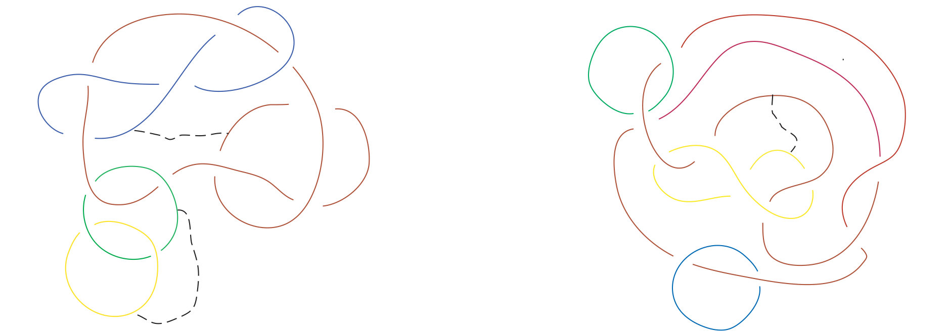 Figure 17
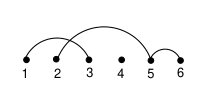 Figure 1
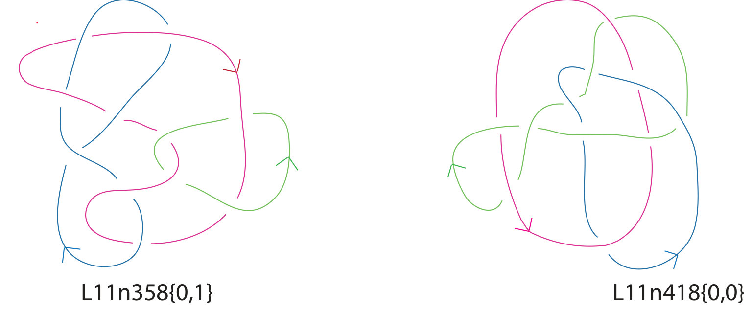 Figure 19
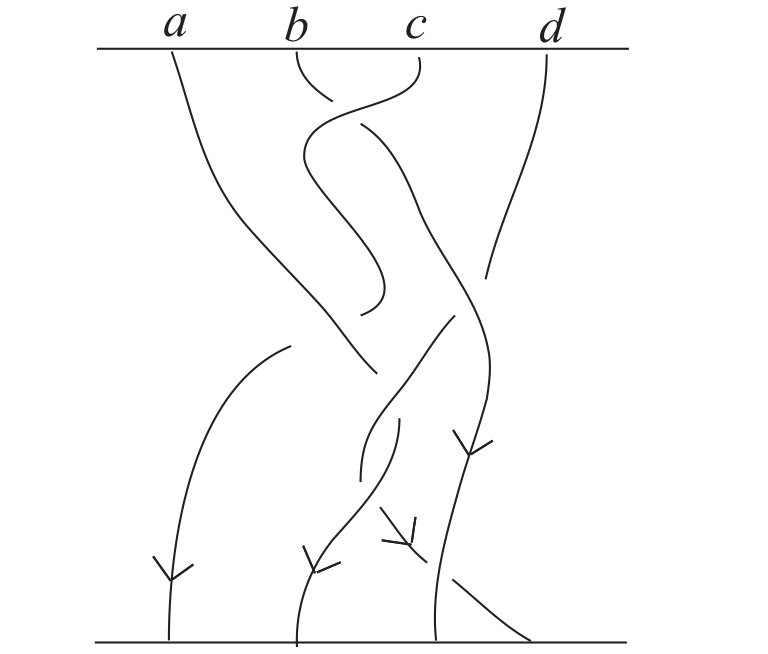 Figure 20
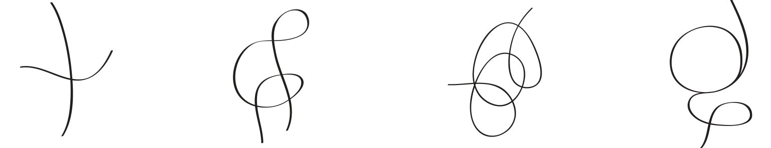 Figure 21
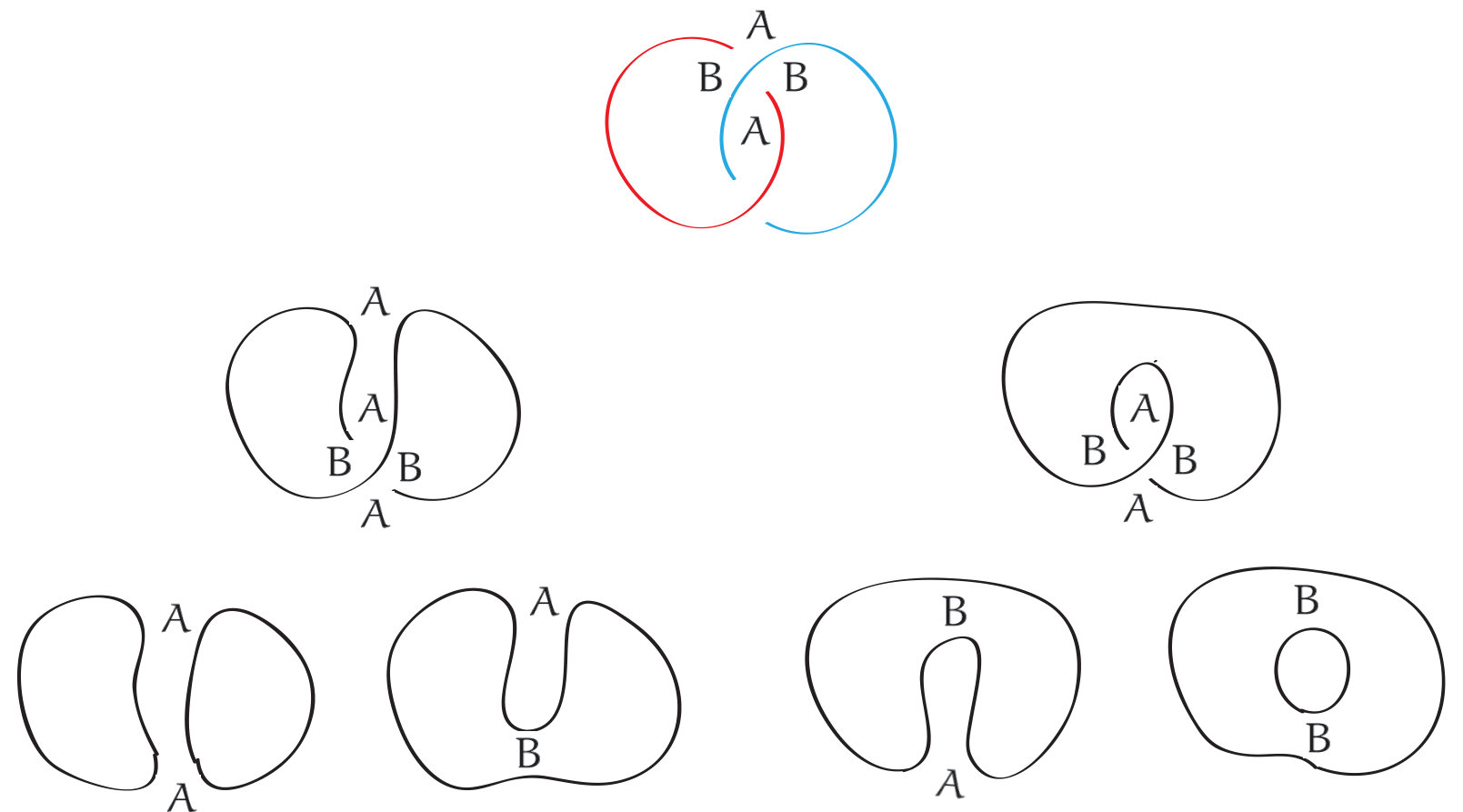 Figure 22
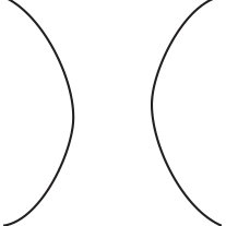 Figure 23
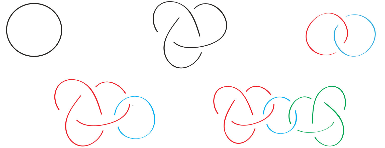 Figure 24
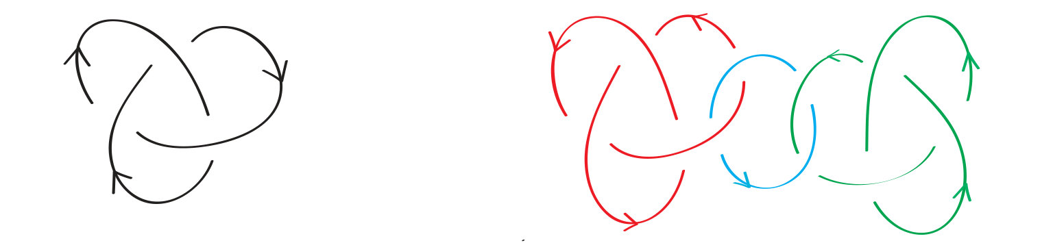 Figure 25
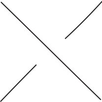 Figure 26
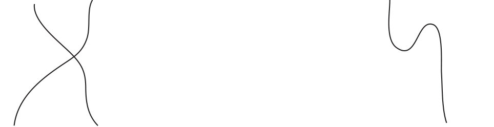 Figure 27
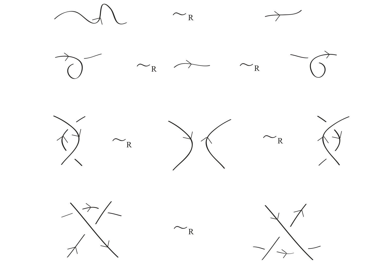 Figure 28
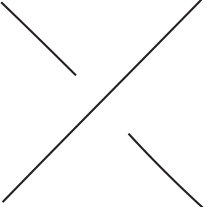 Figure 29
 Figure 30
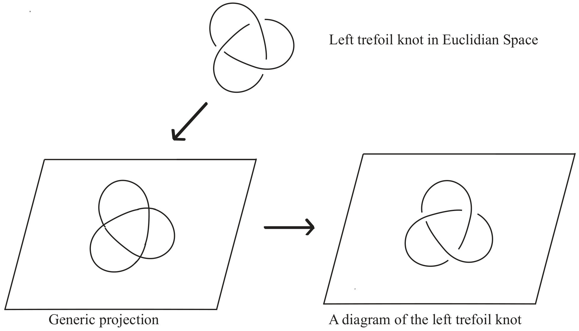 Figure 31
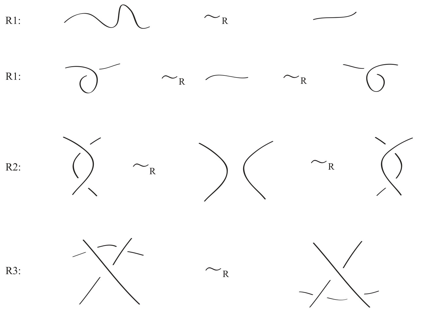 Figure 32
 Figure 33
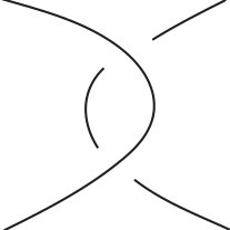 Figure 34
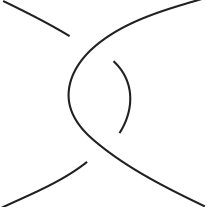 Figure 35
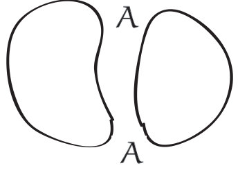 Figure 36
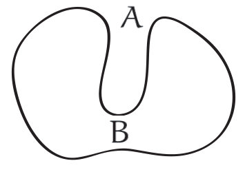 Figure 37
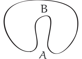 Figure 38
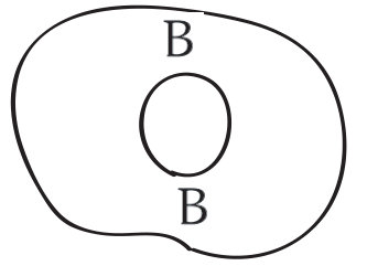 Figure 39
 Figure 40
Peer Reviews
No public reviews on file for this paper yet. If you reviewed it on a platform where reviews are public (OpenReview, ICLR, NeurIPS, ICML), you can paste yours below so the community can read it here.
Videos
No videos yet. Explain this paper in a talk, walkthrough, or lecture? Add one.
Taxonomy
TopicsGeometric and Algebraic Topology · Advanced Combinatorial Mathematics · Advanced Operator Algebra Research
Polynomial invariants for links and tied links
Jesús Juyumaya
IMUV, Universidad de Valparaíso, Gran Bretaña 1111, Valparaíso 2340000, Chile.
Key words and phrases:
Links, diagrams of links, braid group, Hecke algebras
1991 Mathematics Subject Classification:
57M25, 20C08, 20F36
Notes based on lessons given at Escuela ‘Fico González Acuña’ de Nudos y 3-variedades, Mérida Yucatán, México, 7–10 (2015) and Encuentro de nudos, trenzas y álgebras, Oaxaca–México, 3–10 October (2018).
I would like to thank for the invitation and hospitality received from Mario Eudave at Merida and Bruno Cisneros at Oaxaca. Also, I would like to thank Francesca Aicardi and Nicoletta Zar for their contribution in the writing of these notes.
Contents
- 1 Background
- 2 Planar diagrams of links
- 3 Bracket polynomial
- 4 Links via braids
- 5 Hecke algebra
- 6 The Homflypt polynomial
- 7 Hecke algebras in representation theory
- 8 Yokonuma–Hecke algebra
- 9 The –system
- 10 The invariants and
- 11 The bt–algebra
- 12 Tied links
- 13 The invariant
1. Background
Definition 1**.**
A knot is a subset of homeomorphic to . A link is a disjoint union of knots, is called the number of components of the link.
In Fig. 1: the first knot is called the unknot, the second is the left trefoil knot, the third is the Hopf link, the fourth is a link with two components and the fifth is a link with three components.
Since a knot is a simple closed curve we can provide it with an orientation, in such case we say that the knot is oriented. If each component of a link is oriented, we say that the link is oriented.
Definition 2**.**
Two links and (both oriented or not) are called ambient isotopic (or equivalent) if there exists an ambient isotopy of that carries in , that is, there is a continue map such that:
- (1)
* and ,* 2. (2)
For every , the maps ’s are continues and injective, where denotes to restricted to .
The fact that and are ambient isotopic is denoted by .
From now on we denote, respectively, by and the set of all oriented links and unoriented links in .
Proposition 1**.**
The relation is an equivalence relation on .
The main problem in knot theory is to find a subset of representatives of equivalence class of under the relations , or equivalently, given two links to decide if they are ambient isotopic or not. This problem is far from solution; however, we have a tool that helps to decide when two links are not ambient isotopic: the invariant of links.
Definition 3**.**
Let be a set, an invariant of link is a function such that:
[TABLE]
In the case that is a polynomial ring or a field of rational functions, we say that is a polynomial invariant of links.
To have an invariant when is well understood allows to compare easily the images of the links by ; therefore, is useful in the sense that if the images of the links are different then the links are not equivalent. Some famous classical invariants are: the linking number, the 3–coloration, the fundamental group of a link and the following polynomial invariants:
- (1)
The Alexander polynomial, 2. (2)
The Jones polynomial, 3. (3)
The Homflypt polynomial, 4. (4)
The Kauffman polynomial.
The Alexander and Jones invariants are polynomials in one variable. The Homflypt and Kauffman polynomial are in two variables. The Jones polynomial can be obtained as a specialization both of the Kauffman and Homflypt polynomials; the Alexander polynomial can be obtained also as a specialization of the Homflypt polynomial, but not as a specialization of the normalized Kauffman polynomial . We note that all these polynomial invariants are defined for oriented links.
2. Planar diagrams of links
The links can be studied through diagrams in : we associate to each link a generic projection on a plane, this projection is provided with codes to indicate, at every double point, what portion of the projected curve (shadows) is coming from an over or under crossing. Thanks to a theorem of Kurt Reidemeister, the study of links can be translated to the study of diagrams of links, allowing thus a combinatoric treating of the study of links.
Definition 4**.**
A generic projection of a curve of on a plane is one that only admits simple crossings.
In Fig. 3, the first figure is a simple crossing, the second figure is a generic projection of a curve and the third and fourth figures are not generic projections of a curve.
Definition 5**.**
A diagram of a link is a generic projection (or shadow) of it on a plane, where each further simple crossing is codified, depending if it is originated from an over or under crossing in the link, by one of the two crossing codifications below.
More precisely, in Fig. 4, the first picture is a simple crossing in the diagram produced by the projection of the curves and of the link, the second picture shows the code used to indicate that the curve is under the curve in the link and the last picture is to indicate that the curve is over the curve in the link.
Example 1**.**
Fig. 5 shows the procedure to obtain a projection of a left trefoil knot.
Oriented links yields oriented diagrams; thus a diagram is oriented if every crossing codification is in one of the following situations:
The first codification is called (by convention) positive crossing and the other one negative crossing. The sign of the crossing is if it is a positive crossing, otherwise is .
Definition 6**.**
Let be an oriented diagram, the writhe of , denoted by , is the sum over the sign of all crossings of :
[TABLE]
where running on the crossing of and is the sign of the crossing .
Definition 7**.**
*Two diagrams of unoriented links are R–isotopic if one of them can be transformed in the other, by so–called Reidemeister moves *R0, R1, R2 and/or R3, where in the case unoriented links are:
We have the analogous definition for diagrams of oriented links but by adding now all possible orientations to the moves R1–R3 above. For instance, some of these oriented Reidemeister are shown in Fig. 8.
Proposition 2**.**
The relation of R–isotopic, denoted by , defines an equivalence relation on the set of planar diagrams.
Notation 1**.**
- (1)
If is an oriented diagram, we denote by the unoriented diagram obtained by forgetting the orientation in . 2. (2)
We denote, respectively, by and the set of diagrams of, respectively, oriented and unoriented links in .
Theorem 1** (Reidemeister, 1932).**
Let and be two links (oriented or not) and set and diagrams, respectively, of and , we have:
[TABLE]
So, is in bijection with .
Example 2**.**
The Reidemeister theorem says that constructing an invariant of links is equivalent to defining a function , such that it takes the same values on diagrams that differ in R1, R2 and/or R3.
Definition 8**.**
We say that is an invariant of regular isotopy if the values of does not change on unoriented links that are equal, up to the moves and .
Proposition 3**.**
* is an invariant of regular isotopy.*
Proof.
To check that agrees with the oriented move R2, it is enough to observe that introducing any orientation to , it turns out that the sum of the crossing signs is [math]; the same happens with . Also, it is easy to see that by introducing any orientation to one of the crossing configurations of R3, the sum of the signs of the three crossings in it doesn’t change after applying the move R3. ∎
The following lemma gives a recipe, due to L. Kauffman, to produce invariants of oriented links. This recipe was applied to define the Kauffman and Dubrovnik polynomials.
Lemma 1** ([18, Lemma 2.1]).**
Let be a ring and an invertible element of . Suppose that is a regular isotopy invariant of unoriented diagram links taking values in , such that:
[TABLE]
Then, the function defined as
[TABLE]
is an invariant for oriented links, where is a diagram for the oriented link .
3. Bracket polynomial
Let be the diagram of a link. We will attach to a polynomial in the variables , and by using the following inductive process:
- (1)
We consider a crossing of to assign the variables and :
That is, we assign the variable to the region obtained by sweeping the continuous arc in counterclockwise and the variable to the remaining regions. 2. (2)
We smooth the crossing (1) by replacing it with the following two configurations:
We obtain thus two links, say and , to which we assign the marks and respectively. and have both a crossing number less than . 3. (3)
We choose now a crossing in and and we apply again the process (2); then we obtain 4 diagrams with marks and . We apply again this process until we have only links without crossing.
Observe that if the original diagram has –crossings, by applying (1)–(3) we obtain finally diagrams, without crossings, having marks and . We call these diagrams (with their marks) the states of , the set of states of is denoted by .
Example 3**.**
Below the procedure (1)–(3) described above for the Hopf link of Fig. 1.
Given , we denote by the number of components of and by the product (commutative) of the marks appearing in .
Definition 9**.**
The Bracket polynomial of an unoriented diagram , denoted by , is the polynomial in defined by
[TABLE]
Example 4**.**
For the Hopf link, denoted by , we have
[TABLE]
Thus, in this example it seems that in the number of components , then
[TABLE]
Proposition 4**.**
- (1)
, 2. (2)
\left\langle\,\includegraphics[scale={0.12},trim=0.0pt 22.76228pt 0.0pt 0.0pt]{PositiveCrossing.pdf}\,\right\rangle=B\left\langle\,\includegraphics[scale={0.12},trim=0.0pt 22.76228pt 0.0pt 0.0pt]{TanlgeSmothingCrossing.pdf}\,\right\rangle+A\left\langle\,\includegraphics[scale={0.12},trim=0.0pt 22.76228pt 0.0pt 0.0pt]{IdentitySmothingCrossing.pdf}\,\right\rangle, 3. (3)
\left\langle\,\includegraphics[scale={0.12},trim=0.0pt 22.76228pt 0.0pt 0.0pt]{NegativeCrossing.pdf}\,\right\rangle=A\left\langle\,\includegraphics[scale={0.12},trim=0.0pt 22.76228pt 0.0pt 0.0pt]{TanlgeSmothingCrossing.pdf}\,\right\rangle+B\left\langle\,\includegraphics[scale={0.12},trim=0.0pt 22.76228pt 0.0pt 0.0pt]{IdentitySmothingCrossing.pdf}\,\right\rangle.
Proof.
See [19, Proposition 3.2]. ∎
We are going now to study the behaviour of the Bracket polynomial under the Reidemeister moves.
Lemma 2**.**
- (1)
\left\langle\,\includegraphics[scale={0.12},trim=0.0pt 22.76228pt 0.0pt 0.0pt]{SmothingR2.pdf}\,\right\rangle=AB\left\langle\,\includegraphics[scale={0.12},trim=0.0pt 22.76228pt 0.0pt 0.0pt]{IdentitySmothingCrossing.pdf}\,\right\rangle+(A^{2}+B^{2}+ABz)\left\langle\,\includegraphics[scale={0.12},trim=0.0pt 22.76228pt 0.0pt 0.0pt]{TanlgeSmothingCrossing.pdf}\,\right\rangle, 2. (2)
\left\langle\includegraphics[scale={0.2},trim=0.0pt 11.38092pt 0.0pt 0.0pt]{Curler1.pdf}\right\rangle=(Az+B)\left\langle\includegraphics[scale={0.2},trim=0.0pt 11.38092pt 0.0pt 0.0pt]{Curler0.pdf}\right\rangle, 3. (3)
\left\langle\includegraphics[scale={0.2},trim=0.0pt 11.38092pt 0.0pt 0.0pt]{Curler2.pdf}\right\rangle=(Az+B)\left\langle\includegraphics[scale={0.2},trim=0.0pt 11.38092pt 0.0pt 0.0pt]{Curler0.pdf}\right\rangle.
Proof.
See [19, Proposition 3.3]. ∎
According to (1) Lemma 2, in order to obtain that the Bracket polynomial respects the move R2 we must have: and , or equivalently:
[TABLE]
Proposition 5**.**
Under the conditions of (1), the Bracket polynomial agrees with the Reidemeister move R3.
Proof.
See [19, Corollary 3.4]. ∎
Proposition 6**.**
Under the conditions of (1), we have:
- (1)
\left\langle\includegraphics[scale={0.2},trim=0.0pt 11.38092pt 0.0pt 0.0pt]{Curler1.pdf}\right\rangle=-A^{3}\left\langle\includegraphics[scale={0.2},trim=0.0pt 11.38092pt 0.0pt 0.0pt]{Curler0.pdf}\right\rangle, 2. (2)
\left\langle\includegraphics[scale={0.2},trim=0.0pt 11.38092pt 0.0pt 0.0pt]{Curler2.pdf}\right\rangle=-A^{-3}\left\langle\includegraphics[scale={0.2},trim=0.0pt 11.38092pt 0.0pt 0.0pt]{Curler0.pdf}\right\rangle.
Proof.
See [19, Corollary 3.4]. ∎
Denote by the function
[TABLE]
This function is called function Bracket polynomial and is characterized in the following theorem.
Theorem 2**.**
The function Bracket polynomial is the unique function that satisfies:
- (1)
, 2. (2)
, 3. (3)
\left\langle\,\includegraphics[scale={0.12},trim=0.0pt 22.76228pt 0.0pt 0.0pt]{PositiveCrossing.pdf}\,\right\rangle=A\langle\,\includegraphics[scale={0.12},trim=0.0pt 22.76228pt 0.0pt 0.0pt]{IdentitySmothingCrossing.pdf}\,\rangle+A^{-1}\langle\,\includegraphics[scale={0.12},trim=0.0pt 22.76228pt 0.0pt 0.0pt]{TangleSmothingCrossing.pdf}\,\rangle.
3.1.
Let be a diagram of the oriented link , we define as follows:
[TABLE]
Then, thanks to the Lemma 1, we have the following theorem.
Theorem 3** ([18, Proposition 2.5 ]).**
The map is an invariant of oriented links.
Remark 1**.**
By making , we have that becomes the seminal Jones polynomial of oriented links. It is a very interesting point, that such an important modern mathematical object can be constructed in such a simple way.
The invariant is useful to detect if a link is equivalent to that obtained by reflection, also called mirror image. Given a link , its mirror image is the link obtained by reflection of in a plane. Notice that the diagrams of are in bijection with the diagrams of : a diagram of determines the diagram of obtained by exchanging the positive with the negative crossing in .
Definition 10**.**
If and are ambient isotopic we say that the links are amphicheiral, otherwise we say that the links are cheiral.
Example 5**.**
In the first row of the figure below we have, respectively, the Hopf link, the trefoil and the figure–eight. In the second row their respective reflected. The Hopf link and the figure–eight are amphicheiral and the trefoil is cheiral.
Proposition 7**.**
Let an oriented link and a diagram of , we have:
- (1)
, 2. (2)
.
4. Links via braids
Another way to study knot theory is through braids. Braids were introduced by E. Artin and the equivalence between braids and knots is due to two theorems: the Alexander and the Markov theorems. This section is a necessary compilation, for this exposition, on the equivalence between knot theory and braid theory.
Throughout these notes we denote by the symmetric group on symbols and we denote by the elementary transposition . Recall that the Coxeter presentation of , for , is that with generators and the following relations:
[TABLE]
4.1.
Let be points in a plane and points in another plane parallel to the first. A –geometrical braid is a collection of arcs connecting the initial points ’s with the ending points , where , such that:
- (1)
for every different and the arcs and are disjoint, 2. (2)
every plane parallel to the plane containing the points ’s meets each arc in only one point.
Geometrically, the arcs cannot be in the following situations:
Define as the set formed by the –geometrical braids. We define on the equivalence relation, denoted by , given by continues deformation. That is, two geometrical braids and are equivalents if there exists a family of geometrical braids such that and .
As in knot theory we can translate, equivalently, the geometrical braids to diagrams of them. More precisely, a diagram of a geometrical braid is the image of a generic projection of the braid in a plane. Thus, we have the analogous of Reidemeister theorem for braids.
Theorem 4**.**
Two geometrical braids are equivalent by if and only if their diagrams are equivalents, that is, every diagram of one of them can be transformed in a diagram of the other, by using a finite number of times the following replacement:
Notation 2**.**
We shall use also to denote the set of diagrams of –geometrical braids and to denote the equivalence of diagrams of braids.
Now, we can define the ‘product by concatenation’ between –geometrical braids; more precisely, given and in we define by as that one defined by rescaling the result of the –geometrical braid obtained by identifying the ending points of with the initial points of .
Lemma 3**.**
For , , and in such that and , we have .
Proof.
We have and also , then . ∎
Denote by the set of equivalence class of relative to ; thus the elements of are the equivalence classes of . The Lemma 3 allows to pass the product by concatenation of to :
[TABLE]
Theorem 5**.**
* is a group with the product by concatenation.*
From now on we denote simply by . Thus, observe that the identity can be pictured by:
and the inverse of is obtained by a reflection of :
Remark 2**.**
Observe that is the trivial group and is the group of .
For , denote by ’s the following elementary braid:
Theorem 6** (Artin).**
For , can be presented by generators and the following relations:
[TABLE]
An immediate consequence of the above is that we have the following epimorphism:
[TABLE]
Notice that for every we have a natural monomorphism from in , where for every braid , is the braid of coinciding with up to strand and having one more strand with no crossing with the preceding strand.
Notation 3**.**
We denote by the group obtained as the inductive limit of .
4.2.
Given , the identification of the initial points with the end points of determines a diagram of oriented links, which is denoted by ; this process of identification is known as the closure of a braid. Thus we have the ‘function closure’
[TABLE]
The proof that the function closure is epijective is due to Alexander; we will outline this proof, since it gives an efficient method to compute the preimage, by , of a given link.
Theorem 7** (Alexander, 1923).**
Every oriented link is the closure of a braid.
Proof.
The sketch of the proof is as follows. Suppose we have a diagram of an oriented link .
- (1)
We fix a point in the plane not lying on any arc of , such that a point moving along each component of the link is always seen from going counterclockwise (or clockwise). Alexander proved that such a point always exists in the isotopy class of the link diagram of . 2. (2)
We divide the diagram in sectors, by rays starting from , with the condition that each sector contains only one crossing. 3. (3)
Finally, we open the diagram along one of the rays obtaining a braid whose closure is the diagram .
∎
Example 6**.**
Fig. 12 shows that the left trefoil is the closure of the braid .
In order to describe the links through braids we need to know when the closure of two braids yields the same link. In fact the map closure is not injective; for instance the braids and yield the same link. The answer to which braids in yield the same link is due to Markov.
Denote by the equivalence relation on generated by the following replacements (also called moves):
- (1)
M1: can be replaced by (commutation), 2. (2)
M2: can be replaced by or by (stabilization),
where and are in .
The relation defines in fact an equivalence relation in . Two elements in the same –class are called Markov equivalent.
Theorem 8** (Markov).**
For and in , we have: and are ambient isotopic links if and only if and are Markov equivalent.
From the Theorems 7 and 8, it follows that:
Corollary 1**.**
There is a bijection between and defined through the mapping .
Remark 3**.**
The Markov theorem says that constructing an invariant for links is equivalent to defining a map , such that for all and in , agrees with the replacements of Markov M1 and M2, that is, satisfies:
- (1)
, 2. (2)
.
5. Hecke algebra
Let be a field, from now on the denomination –algebra mean an associative unital, with unity 1, algebra over the field ; thus we can regard as a subalgebra of the center of the algebra.
Given a group , we denote by the –algebra known as the group algebra of over . Recall that the set is a linear basis for , regarded as a –vector space. Also recall that if has a presentation , then the –algebra can be presented by generators and the relations in .
5.1.
Let be an indeterminate in and set the field of the rational functions . For , the Hecke algebra, denoted by or simply , is defined by and for as the –algebra presented by generators and the relations:
[TABLE]
The ’s are invertible, indeed we have
[TABLE]
Remark 4**.**
- (1)
Taking as power of a prime number, the Hecke algebra above appears in representation theory as a centralizer of a natural representation associated to the action of the finite general linear group on the variety of flags. This feature of the Hecke algebra will be the key point to construct here certain new invariants of links by using other Hecke algebra or other algebras of type Hecke. Consequently, the next subsection will be devoted to present the Hecke algebras in the context of representation theory capturing in particular the Hecke algebra defined above. 2. (2)
The natural map defines an algebra epimorphism from to . Then, we have that the Hecke algebra is the quotient of by the two sided ideal generator by
[TABLE] 3. (3)
By taking the specialization , the Hecke algebra becomes the group algebra of the symmetric group. For this reason the Hecke algebra is known also as a deformation of the symmetric group.
We construct now a basis of the Hecke algebra; this basis is constructed in an inductive way and is used to prove that the algebra supports a Markov trace. We start with the following lemma.
Lemma 4**.**
In every word in can be written as a linear combination of words in the and the ’s such that each of them contains at most one . Hence, is finite dimensional.
Proof.
The proof is by induction on . For the lemma holds since is the algebra generated by and . Suppose now that the lemma is valid for every , with . We prove the lemma for ; let be a word in containing two times , then we can write
[TABLE]
where ’s are words in . But now, using the induction hypothesis we have to consider two situations according to contains none or only one . If does not contain , we have .; hence , thus is reduced as the lemma claims. On the other hand, if contains only one , we can write it as , where and are words in ; so ; by applying now (5) and (6) we obtain , then is as the lemma claims.
In the case that contains more than two generators , we reduce two of them using the argument above; so arguing inductively we deduce that can be written as the lemma is claiming. ∎
In , define: and , for
Definition 11**.**
The elements , with , are called normal words. This set formed by the normal words will be denoted by .
Observe that:
[TABLE]
Theorem 9**.**
The set is a linear basis of . In particular, the dimension of is .
Proof.
We will prove, by induction on , that is a spanning set of . For the theorem is clear. Suppose now that the theorem is true for every . From Lemma 4 it follows that is linearly spanned by the elements of the form (i) and (ii):
[TABLE]
where ’s are words in . By the induction hypothesis, follows that ’s are linear combination of elements of , so we can suppose that ’s belong to . Thus, it is enough to prove that the elements of (ii) are a linear combination of the elements of (notice that ). Set , where ; we have
[TABLE]
From the induction hypothesis is a linear combination of elements of and notice that . So, having in mind the second observation of (9) we deduce that the elements in (ii) belong to the linear span of .
Linear independency (LATER)
∎
The above theorem and (9) imply that we have a natural tower of algebras
[TABLE]
We will denote by the inductive limit associated to this tower.
Notice that the inclusion of algebras allows to obtain a structure of –bimodule for ; further, we can consider the –bimodule since is a –bimodule and also –bimodule.
Proposition 8**.**
The dimension of the –vector space is at most .
Proof.
Theorem 9 implies that every element in is a –linear combination of elements of the form , where . Now, we have two possibilities: is in or , with (see (9)). Now, if , we have and in the other case we can write . Therefore, every element of is a linear combination of elements of the form and , where and . Hence the proof follows. ∎
The following lemma will be used in the next section.
Lemma 5**.**
The map , defined by
[TABLE]
is an isomorphism of –bimodules.
Proof.
∎
5.2.
From now on denotes a new variable commuting with .
Theorem 10** (Ocneanu).**
There exists a unique family of linear maps , where is defined inductively by the following rules:
- (1)
, 2. (2)
, 3. (3)
,
where .
Proof.
The definition of is based on the homomorphism of Lemma 5. For , is defined as the identity on . Now, given , the Lemma 5 says that, we can write uniquely, , then we define by
[TABLE]
For instance , since .
For every , we have , then the rule (3) is satisfied.
We are going to check now the rule (2) BLABLA… ∎
6. The Homflypt polynomial
We show now the construction of the Homflypt polynomial due to V. Jones. This Jones construction gives a method (or Jones recipe) which is our main tool to construct invariants.
6.1.
We have a natural representation from in , defined by mapping in , however we need to consider a slightly more general representation, denoted by and defined by mapping in , where is a scalar factor; the reason for taking this factor will be clear soon. Now, composing with the Markov trace , we have the maps
[TABLE]
This family of maps yields a unique map from to . Now, according to Remark 3, the function defines an invariant of links, if it agrees with the replacements of Markov M1 and M2, or equivalently, for every the function agrees with M1 and M2. The fact that is a homomorphism and the rule (2) of the Ocneanu trace implies that, for every and the maps agree with the Markov replacement M1. For the replacement M2 we note that, in particular, the maps must satisfy:
[TABLE]
We have and from (8), we get:
[TABLE]
Then we derive that , from where the factor satisfies:
[TABLE]
So, extending the ground field to , the family of maps agrees with the Markov replacements M1 and M2. However, it is desirable that the invariant takes the values 1 on the unknot, that is, we want , for every and every whose closure is the unknot; notice that the unknot is the closure of the braid , for all . So, we have:
[TABLE]
Then, we need to normalize by .
Theorem 11**.**
Let be an oriented link obtained as the closure of the braid . We define , by
[TABLE]
Then is an invariant of ambient isotopy for oriented links.
Proof.
Thanks to Corollary 1, we need only to check that:
[TABLE]
where . Clearly (i) holds. We are going to check now only the second equality of (ii), the checking of first equality is left to the reader. We have:
[TABLE]
Then, by using now the rule (3) of the Ocneanu trace, we get ; hence . ∎
Example 7**.**
Trefoil
6.2.
The Homflypt polynomial has a definition by skein rules. This definition is useful to calculate it and also to study its relations with other invariants such as the Jones polynomial and the Alexander polynomial.
Denote by and three oriented links with, respectively, diagrams and , which are different only inside a disk, where they are respectively placed, as shows Fig 13.
The links and are called a Conway triple; notice that in terms of braids, they can be written as:
[TABLE]
for some braid in .
Keeping the notation above, we are going to compute the Homflypt polynomial on a Conway triple. First, we have,
[TABLE]
by considering now (8), we obtain:
[TABLE]
Also a direct computation yields:
[TABLE]
[TABLE]
From these last three equations we obtain the following proposition.
Proposition 9**.**
The invariant satisfies the following skein relation.
[TABLE]
Theorem 12**.**
There exists a unique function
[TABLE]
such that:
- (1)
, 2. (2)
.
Proof.
After a suitable change of variables, satisfies the defining properties of , so it remains to prove the uniqueness of . ∎
Remark 5**.**
Making the polynomial becomes the Jones polynomial and making the polynomial becomes the Alexander polynomial.
7. Hecke algebras in representation theory
7.1.
Let be a finite group. A complex representation of is a pair , where is a finite dimensional space over and is a homomorphism group from to . A subspace of is called –stable if ; the representation is called irreducible if the unique –stable subspaces are trivial. It is well known that every complex representation can be decomposed as a direct sum of stable subspaces, see [23]. A fundamental problem in representation theory is: given a representation of , write out such a decomposition. A powerful tool that helps the understanding of the decomposition of a representation is its centralizer, that is, the algebra formed by the endomorphisms of commuting with , for all . The centralizer of the representation is denoted by .
Now, given a subgroup of we can construct the so called natural or induced representation, of relative a . More precisely, this representation can be made explicit as , where:
[TABLE]
and
[TABLE]
The centralizer of this representation is known as the Hecke algebra of with respect to and is usually denoted by .
A fundamental piece in the theory of finite group of Lie type is the representation theory of the finite general linear group , where denotes the finite field with elements; and an important family of irreducible representation of appears in the decomposition of , where is the subgroup of formed by the upper triangular matrices. The centralizer of this representation was studied by N. Iwahori in the sixties, in a more general context for : the finite Chevalley groups. In the case is as above, that is, the finite general group, the algebra corresponds to those of type in the classification of Chevalley groups and the Iwahori theorem for is the following.
Theorem 13** (N. Iwahori, [12]).**
The Hecke algebra can be presented, as –algebra, by generators and the following relations:
- (1)
, for all , 2. (2)
, for , 3. (3)
, for .
Now, we want to explain a little bit how the ’s look and work. To better explain we shall work in a more general setting. Let be a finite group and set a finite –space. Define the –vector space of all complex valued functions on . Then, we have the representation of , where . Consider now the –space with action and the vector space , this vector space results to be an algebra with the convolution product:
[TABLE]
Theorem 14**.**
The function from to is an algebra isomorphism, where , is defined by
[TABLE]
Proof.
∎
Recall that denote the centralizer of the representation and denote now by the subalgebra of all , that are –invariant, that is, , for and .
Theorem 15**.**
The algebras and are isomorphic.
Proof.
∎
Let be the orbits of the –space , hence the canonical basis of is , where the ’s are the function delta of Dirac,
[TABLE]
Corollary 2**.**
A basis of is the set , where
[TABLE]
Hence, the dimension of is the number of –orbits of .
Proof.
Notice that , so the proof is clear. ∎
We shall finish the section by showing the basis in the case and the variety of flags in .
Remark 6**.**
In [14, p. 336 ] Jones raised the question whether his method of construction of the Homflypt polynomial can be used for Hecke algebras of other type. In this light it is natural to ask also whether the Jones method can be used still keeping but changing for other notable subgroups of . This is what we did to define new invariants for links. More precisely, we change by his unipotent part, that is, the subgroup formed by the upper unitriangular matrices.
8. Yokonuma–Hecke algebra
In this section we introduce the Yokonuma–Hecke whose origin is in representation theory of finite Chevalley groups; indeed, it appears as a centralizer of a natural representation of a Chevalley group. With the aim to applying this algebra to knot theory, we noted that it is linked, not only to the braid group, but also to the framed braid group. We show an inductive basis, the existence of a Markov trace and the E–system, all that fundamental ingredients to construct our invariants.
8.1.
The Yokonuma–Hecke algebra comes from a centralizer of the permutation representation associated to the finite general linear group with respect to the subgroup consisting of the upper unitriangular matrix, cf. Remark 6. This centralizer was studied by T. Yokonuma who obtained a presentation of it, analogous to that found by N. Iwahori for the Hecke algebra, see Theorem 13. However, the presentation of Yokonuma was slightly modified in order to be applied to knot theory; a little modification of this presentation defines the so called Yokounuma–Hecke algebra.
Definition 12**.**
The Yokonuma–Hecke algebra, in short called Y–H algebra and denoted by , is defined as follows: , and for as the algebra presented by braid generators and framing generators , subject to the following relations:
[TABLE]
where and
[TABLE]
Whenever the variable is irrelevant, we shall denote simply by .
Remark 7**.**
- (1)
The elements ’s result to be idempotents, i.e. and the ’s are invertible,
[TABLE]
These facts will be frequently used in what follows. 2. (2)
Notice that for , the algebra becomes , while for , becomes the group algebra of the cyclic group with elements. 3. (3)
The mapping and , define an homomorphism algebra from onto .
8.2.
We have a natural representation of the braid group in the Y–H algebra since relations (i) and (ii) correspond to the defining relations of the braid group. Moreover, the relations (i)–(iv) correspond to the defining relations of the framing group. To be more precise, the framed braid group, denoted by , is the semi–direct product , where the action that defines the semidirect product is through the homomorphism from onto (see (4)), that is:
[TABLE]
In multiplicative notation the group has the presentation and the direct product has the presentation \langle t_{1},\ldots,t_{n}\;;\;t_{i}t_{j}=t_{j}t_{i}\quad\text{for all i,j}\rangle. Consequently, can be presented by (braids) generators together with the (framing) generators subject to the relations (2), ( 3), , for all and the relations:
[TABLE]
Now, because is a semidirect product, we have that every element in it can be written in the form , where and the ’s are integers called the framing. Further, observe that:
[TABLE]
In diagrams, the element can be represented by the usual diagram braid for together with written at the top of the braid: is placed where the strand starts. For instance, Fig. 14 represents the framed braid .
In terms of diagrams, the formula (21) is translated as follows: we place the diagram of the braid under the diagram of the braid and the framing travels along the strand up to the top of the diagram of , so that the framings of the product are ’s. For instance, for and , the product in terms of diagrams is showed in Fig. 15.
Finally, relations (i)–(v) correspond to the defining relations of the framing module . The –modular framed braid group is the semidirect product ; in other terms, it is the group obtained by imposing the relation to the above presentation of .
8.3.
As for the Hecke algebra, we can construct an inductive basis for the Y–H algebra. To do that, we define in , the following sets:
[TABLE]
and
[TABLE]
Definition 13**.**
Every element in of the form , with , is called normal word. We denote by the set of normal words.
Theorem 16**.**
The set is linear basis for ; hence has dimension .
Observe that every element of has one of the following forms:
[TABLE]
where and .
Example 8**.**
For , we have:
[TABLE]
and
[TABLE]
Thus, of is . The basis of is formed by the elements in the form:
[TABLE]
The elements of the basis of , are of the form:
[TABLE]
We used the underline to indicate the form of (22) for the elements of .
Now, in particular, (22) said that , for all . Then, for every we have the following tower of algebras:
[TABLE]
Notation 4**.**
We denote by the algebra associated to the tower of algebras above.
8.4.
Set and let be independent parameters commuting among them and with the parameters .
Theorem 17**.**
The algebra supports a unique Markov trace, that is, a family of linear maps
[TABLE]
defined uniquely by the following rules:
- (1)
, 2. (2)
, 3. (3)
, 4. (4)
,
where , .
Notice that for the trace becomes the Ocneanu trace.
From now on we fix a positive integer , thus we shall write instead of . Moreover, whenever it is not necessary to explicit , we write simply instead of .
We compute some values of that will be used later. First, we compute , for every .
Notice that by using the rule of commutation . Then, for every , we have:
[TABLE]
Thus . Then,
[TABLE]
Now, we compute .
[TABLE]
Hence for all the trace takes the same values on ; we denote these values by . More generally, we define the elements as follows,
[TABLE]
where the subindices are regarded as module . Then, denoting by , we have
[TABLE]
Notice that .
The following lemmas will be useful in the next section and their proofs are a good example to see how works.
Lemma 6**.**
Set , with . We have
[TABLE]
Proof.
A direct computation shows:
[TABLE]
Then
[TABLE]
so, . Now, . Therefore, the proof follows. ∎
Lemma 7**.**
Set , with . We have
[TABLE]
where .
Proof.
We have to compute firstly the trace of ,
[TABLE]
We have
[TABLE]
where the second equality is obtained by moving to the left. Using first the trace rule (4) and later the trace rule (2), we get
[TABLE]
By using again the trace rule (4), we obtain
[TABLE]
Then,
[TABLE]
∎
9. The –system
The –system is the following non–linear system equation of equation in the variable .
[TABLE]
Example 9**.**
For , the –system is:
[TABLE]
For , the –system is:
[TABLE]
The –system plays a key role to define the invariants in the next section. The –system was solved by P. Gerardin, see [16, Appendix].
Theorem 18** (P. Gerardin, 2013).**
The solutions of the –system are parametrized by the non–empty subset of the group . Moreover, given a such subset , the solutions are:
[TABLE]
Remark 8**.**
Let be a non–empty subset of . We have:
- (1)
For , the solutions of the –system are the –roots of the unity. 2. (2)
If consists of the coprimes with , the solution of the –system are Ramanujan sums. 3. (3)
By taking the parameters trace as a solution of the system, then
[TABLE]
Proposition 10**.**
If the parameters trace ’s are taken as solution of the –system, then for every , we have:
[TABLE]
Proof.
From the linearity of , it is enough to consider in the basis . The proof will be done by induction on . For , the claim is clear since ; suppose now the proposition be true for every and let . Because (22), we have two cases according to the form of : (i) or (ii) , where and .
For the case (i), from Lemma 6 we have: since the ’s are solution of the –system.
For the case (ii), we use the Lemma 7, so: , where . From the inductive hyphotesis we have ; but . Then, .
∎
10. The invariants and
In this section we define the invariants and which are constructed using the method due to V. Jones to construct the Homflypt polynomial, see Section 6. Essentially, in the Jones method we use now the Y–H algebra instead of the Hecke algebra and instead of the Ocneanu trace we use the trace . Observe that the construction below follows what has been done in Section 6.
10.1.
For , we denote by the homomorphism from to , such that . Since is an homomorphism and the trace rule (2) of , it follows that agrees with the Markov replacement M1; thus, it remains to see if agrees with the Markov replacements M2, that is, we need
[TABLE]
Put , then we have and . So, the equation (28) is equivalent to:
[TABLE]
Now, applying the formula (19) to and the linearity of , we get:
[TABLE]
Therefore, in order to get the condition on in (29), we need to factorize by in the second member of the equality of (30). Now, observe that and from (24) we get . Unfortunately, we cannot take out the factor in . However, resorting to Proposition 10, we can do it whenever the ’s are the solution of the E–system. Thus, if is the solution of the –system determined by the set , the equation (30) can be written as
[TABLE]
Then, (29) yields
[TABLE]
So, by (27) we get:
[TABLE]
Because is depending only on the cardinal of , we can define for every , as the above, i.e.
[TABLE]
Recapitulating, by extending the field to , we can consider the following homomorphism ,
[TABLE]
Thus, we have a family of functions agreeing with the replacements M1 and M2. Proceeding as in (11) we get that, now, the factor of normalization for is .
Definition 14**.**
Let . For , we define
[TABLE]
Theorem 19**.**
Let be a link s.t. , where , then the map is an invariant of ambient isotopy for oriented links,
[TABLE]
Remark 9**.**
Regarding (10) and (31) it results clear that is the Homflypt polynomial.
For the benefit of the writing, the main results on the invariant will be established after we define a cousin of , denoted denoted by . These invariants are not equivalents but share several properties.
10.2.
The Yokonuma–Hecke algebra has another presentation due to M. Chlouveraki and L. Poulain d’Andecy [8], cf. [9, 11]. This presentation is constructed as follows. Firstly, the field is extended to with ; secondly, new generators are defined by
[TABLE]
It is a routine to check that the ’s and the ’s satisfy the relations (13)–(17) if one substitutes with and the relation,
[TABLE]
Notice that ’s are invertibles, and
[TABLE]
Thus one obtains a presentation of the Yokonuma–Hecke algebra by the generators ’s and ’s and the same relations of those given for the defining generators ’s and ’s except for the relation (18) which is replaced by the relation (33). We shall use the notation , or simply , whenever the Yokonuma–Hecke algebra is considered with the presentation by the ’s and ’s.
Remark 10**.**
Notice that coincides with the presentation of the Hecke through the generators ’s of Exercise X.
By using now, in the Jones recipe, instead of , one obtains an invariant instead . To be precise, notice firstly that for every , according to properties of , (32) and (24), we have:
[TABLE]
Secondly, given a non–empty subset of and the solutions determined by , for every the Proposition 10 together with (32) and (34,) imply:
[TABLE]
Therefore, the rescaling factor is:
[TABLE]
the last equality is due to (27). Again the rescaling factor depends only on the cardinal , so, by using the procedure used to get the definition of , we get firstly the rescaling factor, denoted by , namely
[TABLE]
and secondly as follows.
Definition 15**.**
For , we define
[TABLE]
Keeping the notations above, we have the following theorem.
Theorem 20**.**
The function , defined by , where is the closure of the braid , is an invariant of ambient isotopy of oriented links.
Remark 11**.**
Exactly as in Remark 9, we have that coincide with the Homflypt polynomial.
Theorem 21**.**
The invariants and coincide with the Homflypt polynomial whenever they are evaluated on knots.
To prove that the invariants and were not equivalents to the Hompflypt polynomial was a not trivial matter. Firstly, in [9] were found six pairs of links with equivalents Homflypt polynomial but different , see [9, Table1]; a such pair is shown in Fig. 16.
Hence.
Theorem 22**.**
For every , the invariants are not equivalent to the Homflypt polynomial.
The people working on theses invariants thought that the invariants and were equivalents111This is due to the fact that in the definitions of and the unique difference is the change of presentations for the Y–H algebra, apparently unimportant thing. but surprisingly F. Aicardi shows that it is not the case.
Theorem 23** (Aicardi).**
For every , the invariants and are not topologically equivalent to the Homflypt polynomial: indeed, there exists pairs of non isotopic links distinguished by and/or but not by the Homflypt polynomial.
Proof.
In [6] we can find several pairs proving this theorem. In Fig. 17, we have a pair of non isotopic links distinguished by , , but neither by Homflypt nor .
∎
The next theorems establish the main properties of the invariants and .
Proposition 11**.**
The invariants and share several properties with the Homflypt polynomial, e.g.: the behavior under connected sums and mirror image.
In the next section we generalize, respectively, the invariants and to, respectively, certain invariants in three parameters, and for classical links. We will do this, by using the Jones recipe applied to the bt–algebra. Also we will see, that can be defined through skein relations, while cannot.
11. The bt–algebra
In this section we introduce the so–called bt–algebra (or algebra of braids and ties) which is constructed by abstracting the braid generators ’s of the Yokonuma–Hecke algebra and the idempotents ’s appearing in the square of the braid generators, see (18). This algebra is used to generalize the invariants and to invariants with three parameters as well as its understanding by skein relations. Before introducing the bt–algebra we shall recall the main facts on set partitions since these facts will be useful in the rest of these notes.
11.1.
For , we denote by the set and by the set formed by the set partitions of , that is, an element of is a collection of pairwise–disjoint non–empty sets whose union is ; the sets are called the blocks of ; the cardinal of , denoted , is called the Bell number.
We can regard as subset of through the natural injective map , where for , the image is defined by adding to the block .
Typically, the set partitions are represented by scheme of arcs, see [20, Subsection 3.2.4.3], that is: the point is connected by an arc to the point , if is the minimum in the same block of satisfying . Figure 18 shows the set partition as represented by arcs.
The representation by arcs of a set partition induces a natural indexation of its blocks. More precisely, we say that the blocks ’s of the set partition of are standard indexed if , for all . For instance, in the set partition of Figure 18 the blocks are indexed as: , and .
The natural action of on induces, in the obvious way, an action of on that is, for we have
[TABLE]
Notice that this action preserves the cardinal of each block of the set partition.
Now, we shall say that two set partitions and in are conjugate, denoted by , if there exists such that, ; if it is necessary to precise such , we write . Further, observe that if and are standard indexed with blocks, then the permutation induces a permutation of of the indices of the blocks, which we denote by
Example 10**.**
Let and
[TABLE]
so and . We have , where:
[TABLE]
Given a permutation and writing as product of disjoint cycles, we denote by the set partition whose blocks are the cycles ’s, regarded now as subsets of . Reciprocally, given a set partition of we denote by an element of whose cycles are the blocks ’s. Moreover, we shall say that the cycles of are standard indexed, if they are indexed according to the standard indexation of .
Notation 5**.**
When there is no risk of confusion, we will omit in the partitions the blocks with a single element.
is a poset with structure of commutative monoid. Indeed, the partial order on is defined as follows: if and only if each block of is a union of blocks of . The product , between and is defined as the minimal set partition, containing and , according to ; the identity of this monoid is . Observe that:
[TABLE]
[TABLE]
Further, the injective maps ’s result to be a monoid homomorphisms and respect , that is, for every , we have:
[TABLE]
Notation 6**.**
The inductive limit associated to the family of monoids is denoted by ,
We are going to give an abstract description of , that is, via a presentation which will be used in the next section. For every with , define as the set partition whose blocks are and where and . We shall write instead of .
Proposition 12**.**
The monoid can be presented by the set partitions ’s subject to the following relations:
[TABLE]
11.2.
The original definition of the bt–algebra is the following.
Definition 16** (See [1, 22, 3]).**
The bt–algebra , denoted by , is defined by and for as the unital associative –algebra, with unity , defined by braid generators and ties generators subjected to the following relations:
[TABLE]
The ’s are invertible, with given by:
[TABLE]
Remark 12**.**
- (1)
The bt–algebra can be seen as a generalization of the Hecke algebra since by making , the definition of the bt–algebra becomes the Hecke algebra. Further, observe that the mapping and defines an epimorphism from the bt–algebra to the Hecke algebra. 2. (2)
The mapping and defines an algebra homomorphism from the bt–algebra to the YH–algebra, which is injective if and only if , see [11], cf. [3, Remark 3].
Diagrammatically the generators ’s can be regarded as usual braids and the generator as a tie between the and strands, this tie doesn’t have a topological meaning: it is an auxiliary artefact to reflect the monomial–homogeneous defining relation of the bt–algebra. Thus, the tie is pictured as a spring or a dashed line between the strands. More precisely, the diagrams for, respectively, and , are:
Here comment!
11.3.
The bt–algebra is a finite dimensional algebra. Moreover, there is a basis due to S. Ryom–Hansen [22]. Before expliciting the Ryom–Hansen basis we need to introduce the tools below.
For , we define by
[TABLE]
For any nonempty subset of we define for and otherwise by
[TABLE]
Note that . For , we define by
[TABLE]
Now, if is a reduced expression of , then the element is well defined. The action of on is inherited from the ’s and we have:
[TABLE]
Theorem 24** ([22, Corollary 3]).**
The set is a –linear basis of . Hence the dimension of is .
Example 11**.**
Having in mind (39), the natural inclusion , for every , together with Theorem 24, we deduce the tower of algebras:
[TABLE]
Notation 7**.**
Denote by the inductive limit associated the bt–algebras above.
Remark 13** (Cf. Subsection 10.2).**
Extending the field to with , we can define (cf. [21, Subsection 2.3]):
[TABLE]
Then the ’s and the ’s satisfy the relations (43)–(48) and the quadratic relation (49) is transformed in
[TABLE]
So,
[TABLE]
In [9, 11, 13] this quadratic relation is used to define the bt–algebra. Although at algebraic level these algebras are the same, we will see that they lead to different invariants. Thus, in order to distinguish these two presentations of the bt–algebra, we will write when the bt–algebra is defined by using the quadratic relation (55).
11.4.
In [3] it was proved that the bt–algebra supports a Markov trace, this was proved using the method of relative trace and the Ryom–Hansen basis.
Let and be two variables commutative independent commuting with .
Theorem 25** ([3, Theorem 3]).**
There exists a unique Markov trace on , i.e., a family , where ’s are linear maps, defined inductively, from in such that and satisfying, for all , the following rules:
- (1)
, 2. (2)
, 3. (3)
.
With this theorem and because the braid group is represented (naturally) in the bt–algebra we are ready to define an invariant for links. More precisely, denote by the (natural) representation of in , namely . With the same procedure used to get (10) and (31), we define
[TABLE]
Definition 17**.**
For , we define
[TABLE]
Theorem 26**.**
Let be a link obtained by closing the braid . Then the map defines an ambient isotopy invariant for oriented links, taking values in .
Proof.
We need only to prove that agrees with the Markov replacements. Because is an homomorphism and the properties of imply that agrees with M1. On the second replacement, we note that it is a routine to check . Thus it remains only to check , for every . Now, put , then:
[TABLE]
Therefore, , for all . ∎
Now, in the way we define we can define , that is, taking out its definition by using now the presentation of the bt–algebra in the Jones recipe. Having in mind what we did above, (35) and Definition 15, we define and as follows:
[TABLE]
[TABLE]
Theorem 27**.**
Let be a link obtained by closing the braid . Then the map defines an invariant of ambient isotopy for oriented links, which take values in .
Proof.
Same proof as Theorem 26. ∎
Remark 14**.**
The invariant contains the invariant , for every ; that is specializing the variable to we get . With the same specialization, the invariant contains the invariants , for every .
12. Tied links
In this section we introduce the tied links. This class of knotted-like objects contains the classical link, so invariants of tied links yield invariants of classical links. We start the section recalling the definition of tied links and the monoid of braid tied links. Also, the respective Alexander and Markov theorems are exhibited.
12.1.
Tied links were introduced in [2] and roughly correspond to links whose components may be connected by ties; thus ties are connecting pairs of points of two components or of the same component.
The ties in the picture of the tied links are drawn as springs or dashed lines, to outline that they can be contracted and extended, letting their extremes to slide along the components.
Notation 8**.**
We will use the notation to indicate that either there is a tie between the components and of a link, or and are the extremes of a chain of components , such that there is a tie between and , for .
Definition 18** ([2, Definition 1.1]).**
Every 1–link is by definition a tied 1–link. For , a tied –link is a link whose set of components is partitioned into parts according to: two components and belong to the same part if .
Notation 9**.**
We denote by the set of oriented tied links.
In Fig. 21 two tied links with four components; moreover, if is the blue component, the red component, the yellow components and the green component, then the partition associated to the first tied link is and the partitions associated to the second tied link is .
Notice that a tied –link , with components’ set , determines a pair in , where and belong to the same block of , if .
Example 12**.**
For instance in Fig. 21, the set partition determined by the first tied link is and the set partition determined by the second tied link is . The set partition determined by the tied link of Fig. 20 is .
Definition 19** (Cf. [2, Definition 1.6]).**
A tie of a tied link is said essential if it cannot be removed without modifying the partition , otherwise the tie is said unessential.
Notice that between the components indexed by the same block of the set partition, the number of essential ties is ; for instance, in the tied link of Fig. 21, left, among the three ties connecting the first three components, only two are essential. The number of unessential ties is arbitrary. Ties connecting one component with itself are unessential.
Definition 20**.**
The –tied link and the –tied link with, respectively, components and , are t–isotopic if:
- (1)
The links and are ambient isotopic (hence . 2. (2)
The set partitions and satisfy , where is the bijection from to induced by the isotopy.
Example 13**.**
In the Fig. 22, we have that and are not t–isotopic. Indeed, the set partition, respectively, of and are and and , but .
Now, has associated the set partition and has associated the set partition and ; thus, . Then, and are t–isotopic
Remark 15**.**
The Definitions 18 and 20 not only say that classical links are included in tied links but also that the classical links can be identified to the set of tied links which components are all tied. Both ways to see the classical links allows to study the isotopy of links through the t–istopy of tied links. Observe that for –tied links with set of components , we have is if it has all components tied and is if does not have ties or has only ties that are unessential.
Remark 16**.**
Everything established for tied links can be translated in terms of diagrams in the obvious way. Informally, it is enough to change ‘links’ by ‘diagrams of a link’ and so on.
12.2.
The classical theorems of Alexander and Markov in knot theory have their analogous in the world of tied links. The starting point to establish these theorems for tied links is the so–called tied braid monoid.
Definition 21**.**
[2, Definition 3.1]* The tied braid monoid is the monoid generated by usual braids and the tied generators , such the ’s satisfy braid relations among them together with the following relations:*
[TABLE]
We denote the inductive limit determined by the natural monomorphism monoid from into .
Diagrammatically, as usual, is represented as the usual braid and the tied generator , as the diagram of , that is, a tie connecting the with –strands, see Fig. 19.
The tied braid monoid is to the bt–algebra as the braid group is to the Hecke algebra. In particular, we have the following proposition and its corollary.
Proposition 13**.**
The mapping , defines an homomorphism, denoted by , from to .
Proof.
∎
Corollary 3**.**
* The bt–algebra is a quotient of . More precisely,*
[TABLE]
where is the two–sided ideal generated by , for .
has a decomposition like semidirect product of groups, this decomposition allows a study purely algebraic–combinatorics of the tied link, see [5], and will be used below. To establish this decomposition, we start by noting that the action of on , see (36), together with the natural projection of (4), define an action of on . We denote by , the action of the braid on , that is, is the result of the application of the permutation to the set partition . Define now the following product in :
[TABLE]
with this product is a monoid, which is denoted by . We shall denote instead .
Theorem 28** ([5, Theorem 9]).**
The monoid and are isomorphic.
Now, as for braid, we can define the closure of a tied braid in the same way of the closure of the braids. Evidently, the closure of a tied braid is a tied link. Moreover, in [2, Theorem 3.5] we have proved the Alexander theorem for tied links; namely.
Theorem 29** ([2, Theorem 3.5]).**
Every oriented tied link can be obtained as closure of a tied braid.
Before establishing the Markov theorem for tied links, notice that according to Theorem 28, every element in can be written uniquely in the form , where and . We use this fact in the definition of Markov moves for tied links and also we use the notation of the ’s as in (40).
Definition 22**.**
We say that are t–Markov equivalents, denoted , if can be obtained from by using a finite sequence of the following replacements:
- tM1.
t–Stabilization: for all , we can replace by , if belong to the same cycle of . 2. tM2.
Commuting in . For all , we can replace by , 3. tM3.
Stabilizations: for all , we can replace by or
The relation is an equivalence relation on and in [2, Theorem 3.7], cf. [5, Theorem 5], the following theorem was proved.
Theorem 30**.**
Two tied links define t–isotopic tied links if and only if they are t–Markov equivalents.
Remark 17**.**
The Markov replacements and are the classical Markov moves but including now the ties, so their geometrical meaning is clear. The replacement tM1 says that the ties provided by in the closure of become unessential ties, so the closure of and defines the same set partition.
13. The invariant
We will define the invariant for tied links. This invariant is of type Homflypt since evaluated on classical links coincide with the Homflypt polynomial. We start by defining it by skein relations and later their definition by the Jones recipe.
13.1.
To define by skein relations we need, as in (13), to introduce the following notation: and denote oriented tied links which have, respectively, oriented diagrams of tied links and , that are identical outside a small disk into which enter two strands, whereas inside the disk the strands look, respectively, as Fig. 23 shows.
We shall call and a tied Conway triple.
Set a variable with unique condition that commutes with and .
Theorem 31** ([2, Theorem 2.1]).**
There is a unique function , defined by the rules:
- (1)
, 2. (2)
For all tied link ,
[TABLE] 3. (3)
The Skein rule:
[TABLE]
Proposition 14**.**
The defining skein relation of is equivalent to the following skein rules:
- (1)
[TABLE] 2. (2)
[TABLE] 3. (3)
[TABLE]
Proof.
∎
Define the set of tied links with all components tied.
Proposition 15**.**
The restriction of to , is determined uniquely by the rules:
- (1)
, 2. (2)
Skein relation on tied Conway triple , and ,
[TABLE]
where and .
Proof.
The computation of on a such tied link can be realized by rules (1) Theorem 31 and the skein relation (1) Proposition 14. Multiplying this skein relations by , we get the values of and . Hence the proof is concluded. ∎
Remark 18**.**
According to Remark 15, is identified to classical links, so, the above proposition and Theorem(12)) say that and Homflypt polynomial coincide on classical links. For this reason we say that is invariant of type Homflypt.
Proposition 16**.**
The restriction of to classical links is more powerful than the Homflypt polynomial.
Proof.
∎
13.2.
In order to define through the Jones recipe, we extend first the domain to ; we denote this extension by . Secondly, we define by
[TABLE]
Theorem 32**.**
Let be a tied link obtained as the closure of the tied braid , then
[TABLE]
The relation among, , and parameters trace and of , is given by the equation:
[TABLE]
The reference list from the paper itself. Each links out to its DOI / PubMed record.
- 1[1] F. Aicardi, J. Juyumaya, An algebra involving braids and ties , ICTP Preprint IC/2000/179. See https://arxiv.org/pdf/1709.03740.pdf.
- 2[2] F. Aicardi and J. Juyumaya, Tied Links , J. Knot Theory Ramifications, 25 (2016), no. 9, 1641001, 28 pp.
- 3[3] F. Aicardi and J. Juyumaya, Markov trace on the algebra of braid and ties , Moscow Math. J. 16 (2016), no. 3, 397–431.
- 4[4] F. Aicardi and J. Juyumaya, Kauffman type invariants for tied links , Math. Z. (2018) 289:567–591.
- 5[5] F. Aicardi and J. Juyumaya, Ties links and invariants for singular links . See ar Xiv:1807.10071.
- 6[6] F. Aicardi, New invariants of links from a skein invariant of colored links , ar Xiv:1512.00686.
- 7[7] J.C. Cha, C. Livingston, Link Info: Table of Knot Invariants , http://www.indiana.edu/linkinfo, April 16, 2015.
- 8[8] M. Chlouveraki, L. Poulain d’Andecy, Representation theory of the Yokonuma–Hecke algebra , Advances in Mathematics 259 (2014), 134–172.