Filaments of galaxies and Voronoi diagrams
Lorenzo Zaninetti

TL;DR
This paper explores the distribution of galaxy clusters by analyzing intersections of Voronoi polyhedrons with spherical shells, linking geometric structures to cosmological models and galaxy clustering.
Contribution
It introduces a method to identify galaxy cluster nodes via Voronoi diagram intersections within a cosmological context.
Findings
Nodes correspond to potential galaxy clusters.
Method aligns with LCDM cosmology predictions.
Provides a geometric approach to galaxy distribution analysis.
Abstract
The intersections between a spherical shell and the faces of Voronoi's polyhedrons are numerically evaluated. The nodes of these intersections are the points that share the same distances from three nuclei. The nodes are assumed to be the places where we will find clusters of galaxies. The cosmological environment is given by the coupling between the number of galaxies as function of the redshift and the LCDM cosmology.
Click any figure to enlarge with its caption.
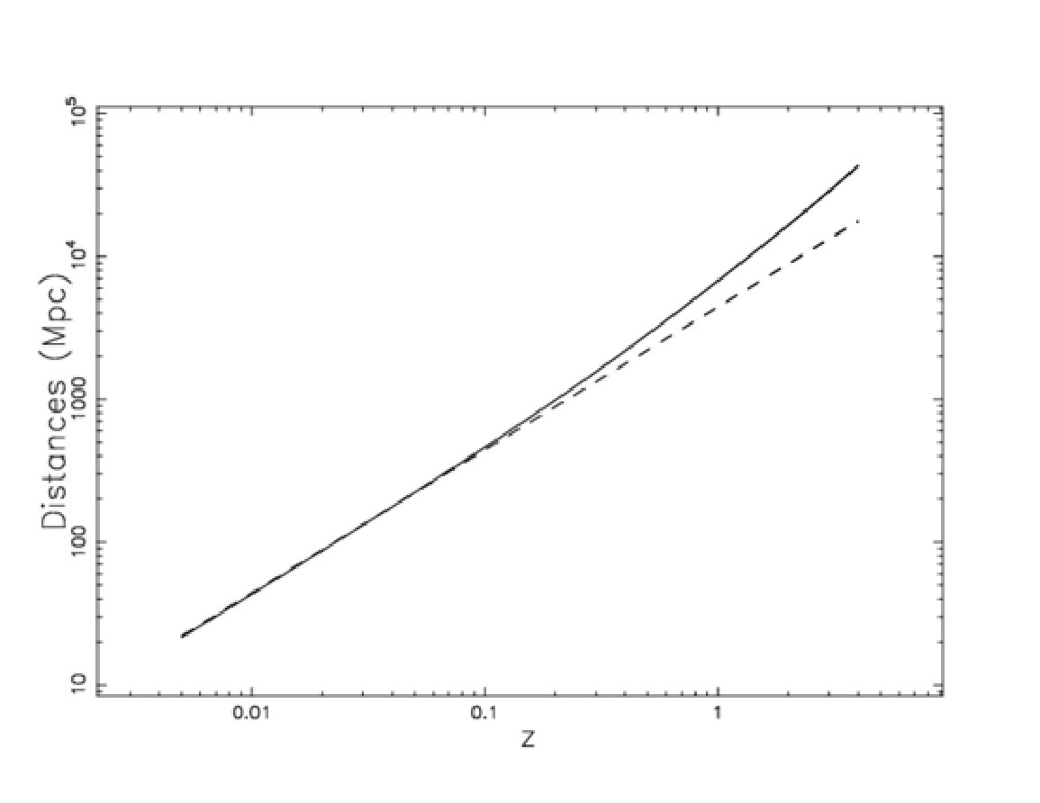 Figure 1
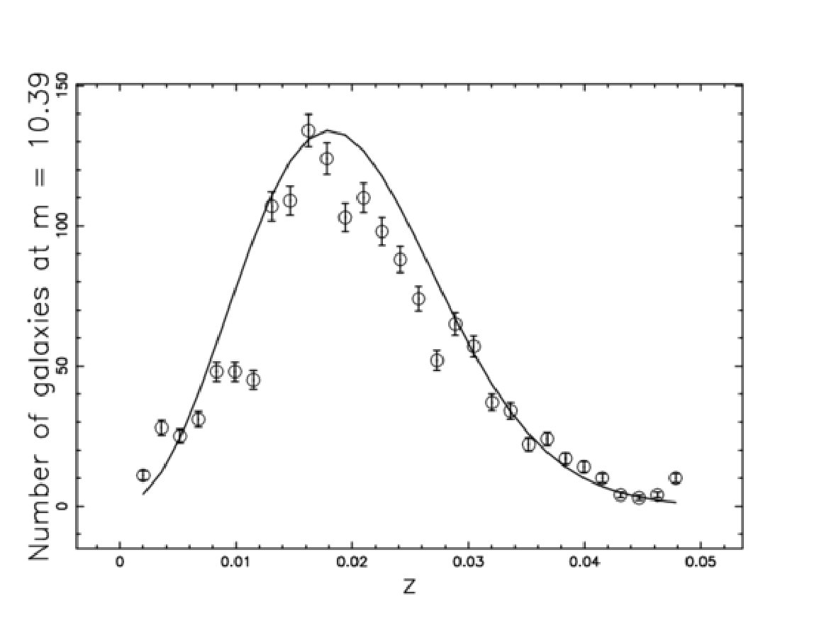 Figure 2
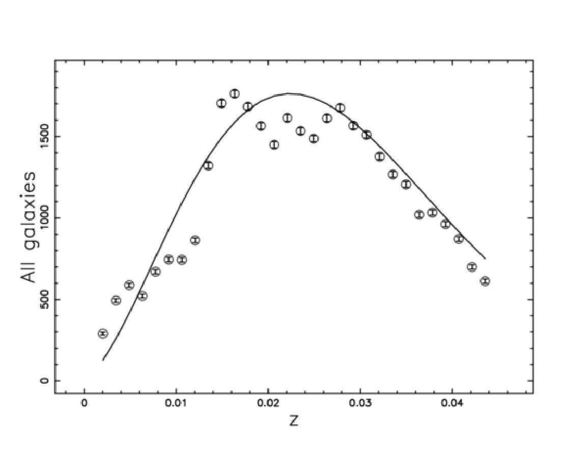 Figure 3
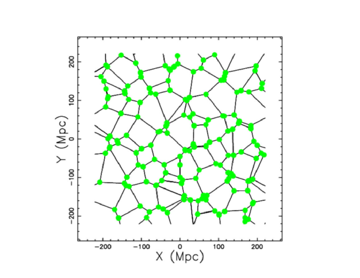 Figure 4
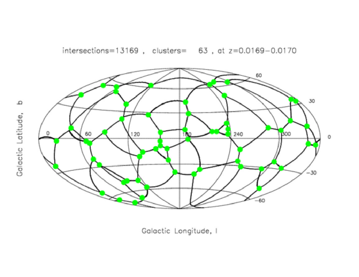 Figure 5
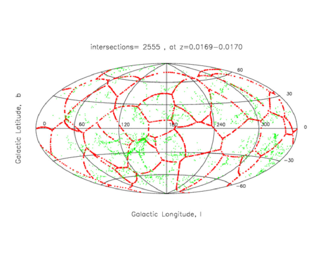 Figure 6
 Figure 7
 Figure 8
 Figure 9
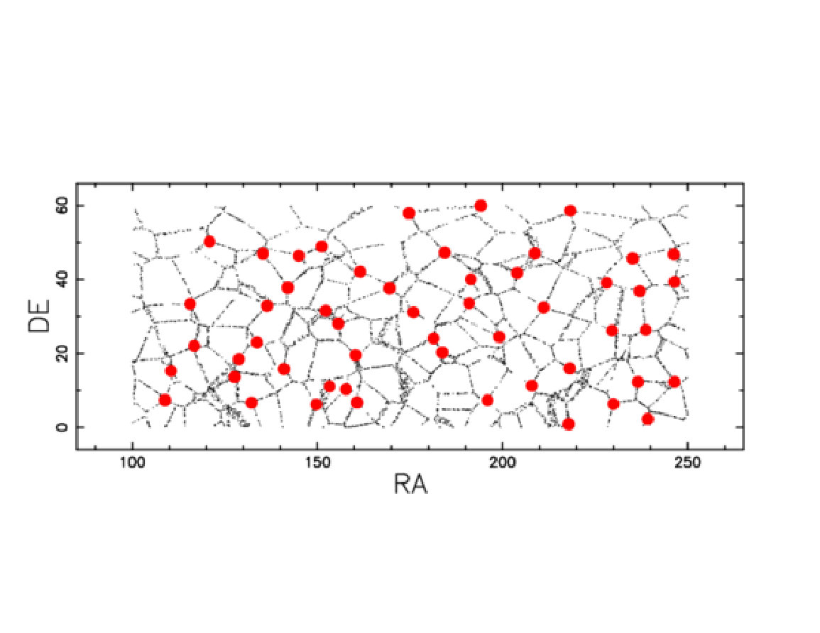 Figure 10
Peer Reviews
No public reviews on file for this paper yet. If you reviewed it on a platform where reviews are public (OpenReview, ICLR, NeurIPS, ICML), you can paste yours below so the community can read it here.
Videos
No videos yet. Explain this paper in a talk, walkthrough, or lecture? Add one.
plus1sp
[1]Lorenzo Zaninetti
L. Zaninetti 11affiliationtext: Physics Department, via P.Giuria 1,
I-10125 Turin,Italy
Filaments of galaxies and Voronoi diagrams
Abstract
The intersections between a spherical shell and the faces of Voronoi's polyhedrons are numerically evaluated. The nodes of these intersections are the points that share the same distances from three nuclei. The nodes are assumed to be the places where we will find clusters of galaxies. The cosmological environment is given by the coupling between the number of galaxies as function of the redshift and the LCDM cosmology.
1 Introduction
The first catalog of clusters of galaxies contained 2712 clusters Abell1958. The updated version brought the number of rich clusters to 4073, each having at least 30 members Abell1989. The second catalog of galaxies contained 29418 galaxies and 9134 clusters and was organized in six books Zwicky1; Zwicky2; Zwicky3; Zwicky4; Zwicky5; Zwicky6. The online version of the Zwicky catalog of galaxies contains 19369 galaxies Falco1999. Another line of research organized the observations of galaxies in slices; the first being the second CFA2 redshift Survey Huchra1999. Other catalogs made by slices or which can be organized in slices are: the 2dfGRS Norberg2002; the 6dF Galaxy Survey 6dFGS Jones2004); and the SDSS DR12 with 208,478,448 galaxies Alam2015. All these slices present filaments of galaxies, which points toward a cellular structure for the 3D spatial distribution of galaxies. A model for the cellular structure of the local universe can be represented in Voronoi Diagrams icke1987; Weygaert1989. In this model the galaxies can be inserted on the faces of irregular polyhedrons Zaninetti1991; zaninetti95. Recently, the analysis of filaments of galaxies with the Cosmic Web Reconstruction (CWR) has made enormous progress Chen2015a; Chen2015b; Chen2016; Chen2017.
The rest of this paper is structured as follows. Section LABEL:section_cosmology introduces the adopted cosmological framework. Section LABEL:section_voronoi models the intersection between a sphere and the network of the Voronoi's faces. Finally, Section LABEL:section_astro reports on the theoretical filaments and clusters of galaxies at low and high values of redshift.
2 Adopted Cosmology
section_cosmology This section introduces two catalogs of galaxies (the CDM and the pseudo-Euclidean cosmology), the statistics of the cosmic voids and the standard luminosity function (LF) for galaxies.
2.1 The adopted catalogs
The 2MASS Redshift Survey (2MRS) has 44599 galaxies between and covers of the sky, see Huchra2012. The redMaPPer catalog has 25000 clusters of galaxies between and covers of the sky, see Rykoff2014.
2.2 Luminosity distance
We review the existing knowledge on the luminosity distance, , which in the CDM cosmology can be expressed in terms of a Padé approximant. We should provide: the Hubble constant, , as expressed in ; the velocity of light, , as expressed in ; and the three numbers , , and , (see Zaninetti2016a for more details). A numerical analysis of the distance modulus for the Union 2.1 compilation, see Suzuki2012, gives , and . We now apply the minimax rational approximation, which is characterized by two parameters and , and we find a simplified expression for the luminosity distance, , when and
[TABLE]
This equation can be inverted to give a "new" expression for the redshift as a function of the luminosity distance in Mpc
[TABLE]
The most simple model for the distance, , in the local universe is that of the pseudo-Euclidean cosmology:
[TABLE]
where we used , see Zaninetti2016c.
The differences between the two distances are the luminosity distance and the and the pseudo-Euclidean distance, which can be outlined in terms of a percentage difference: . For example, for ,
[TABLE]
Figure LABEL:distances reports the two distances. For , the percentage difference is lower than .
Therefore the boundary between low and high can be fixed at .
2.3 Cosmic voids
A first catalog of cosmic voids can be found in Vogeley2012, where the effective radius of the voids, , has been derived
[TABLE]
The second catalog is that of radii up to redshift in (SDSS-DR7), see Varela2012,
[TABLE]
The third catalog is that of the Baryon Oscillation Spectroscopic Survey, see Mao2017,
[TABLE]
In the following, we will calibrate our code on the average value of the three previous values: .
2.4 The LF for galaxies
We now review the actual knowledge on the Schechter function, see schechter which provides a useful standard for the LF of galaxies
[TABLE]
where sets the slope for low values of luminosity, , is the characteristic luminosity and is the normalisation. The equivalent distribution in absolute magnitude is
[TABLE]
where is the characteristic magnitude as derived from the data. The scaling with is and . According to formula(1.104) in pad or formula(1.117) in Padmanabhan_III_2002 , the joint distribution in redshift, z, and flux, f, for galaxies in the pseudo-Euclidean cosmology, is
[TABLE]
where , and represent the differential of the solid angle, the redshift and the flux, respectively, and is the Schechter LF. The critical value of , , is
[TABLE]
The number of galaxies in and as given by formula(LABEL:nfunctionzschechter) has a maximum at , where
[TABLE]
which can be re-expressed as
[TABLE]
where M_{\hbox{\odot}} is the reference magnitude of the sun at the considered bandpass. On replacing the flux with the apparent magnitude
[TABLE]
Figure LABEL:maximum_2mrs reports the number of observed galaxies of the 2MRS catalog for a given apparent magnitude and for the theoretical curve. Table LABEL:parameterslf reports the parameters that were adopted in this model.