Displaying trees across two phylogenetic networks
Janosch D\"ocker, Simone Linz, and Charles Semple

TL;DR
This paper investigates the computational complexity of comparing the display sets of two phylogenetic networks, revealing NP-completeness and $ ext{P}^{ ext{NP}}_{||}$-completeness results for key problems in phylogenetics.
Contribution
It establishes the hardness of determining common trees and equality of display sets for two phylogenetic networks, including the first proof of $ ext{P}^{ ext{NP}}_{||}$-completeness for these problems.
Findings
Deciding if two networks share a common displayed tree is NP-complete.
Checking if two networks have identical display sets is $ ext{P}^{ ext{NP}}_{||}$-complete in general.
Some special cases allow polynomial-time solutions, but the general problems are computationally hard.
Abstract
Phylogenetic networks are a generalization of phylogenetic trees to leaf-labeled directed acyclic graphs that represent ancestral relationships between species whose past includes non-tree-like events such as hybridization and horizontal gene transfer. Indeed, each phylogenetic network embeds a collection of phylogenetic trees. Referring to the collection of trees that a given phylogenetic network embeds as the display set of , several questions in the context of the display set of have recently been analyzed. For example, the widely studied Tree-Containment problem asks if a given phylogenetic tree is contained in the display set of a given network. The focus of this paper are two questions that naturally arise in comparing the display sets of two phylogenetic networks. First, we analyze the problem of deciding if the display sets of two phylogenetic networks have a tree in…
Click any figure to enlarge with its caption.
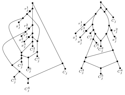 Figure 1
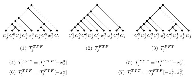 Figure 2
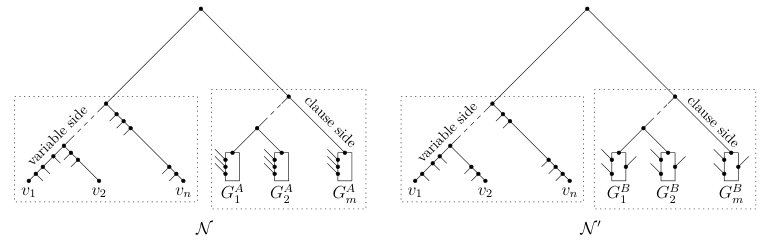 Figure 3
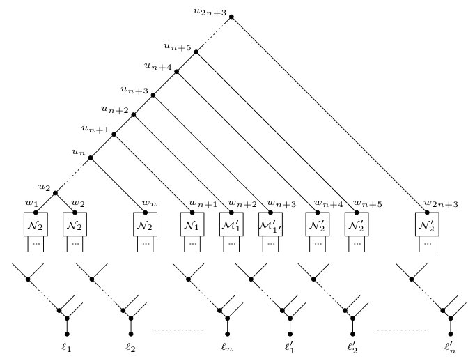 Figure 4
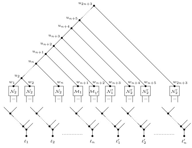 Figure 5
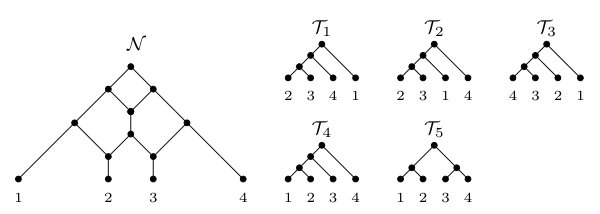 Figure 6
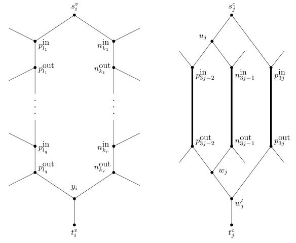 Figure 7
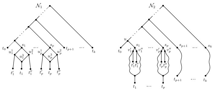 Figure 8
Peer Reviews
No public reviews on file for this paper yet. If you reviewed it on a platform where reviews are public (OpenReview, ICLR, NeurIPS, ICML), you can paste yours below so the community can read it here.
Videos
No videos yet. Explain this paper in a talk, walkthrough, or lecture? Add one.
Displaying trees across two phylogenetic networks
Janosch Döcker, Simone Linz, and Charles Semple
Department of Computer Science, University of Tübingen, Tübingen, Germany
School of Computer Science, University of Auckland, Auckland, New Zealand
School of Mathematics and Statistics, University of Canterbury, Christchurch, New Zealand
Abstract.
Phylogenetic networks are a generalization of phylogenetic trees to leaf-labeled directed acyclic graphs that represent ancestral relationships between species whose past includes non-tree-like events such as hybridization and horizontal gene transfer. Indeed, each phylogenetic network embeds a collection of phylogenetic trees. Referring to the collection of trees that a given phylogenetic network embeds as the display set of , several questions in the context of the display set of have recently been analyzed. For example, the widely studied Tree-Containment problem asks if a given phylogenetic tree is contained in the display set of a given network. The focus of this paper are two questions that naturally arise in comparing the display sets of two phylogenetic networks. First, we analyze the problem of deciding if the display sets of two phylogenetic networks have a tree in common. Surprisingly, this problem turns out to be NP-complete even for two temporal normal networks. Second, we investigate the question of whether or not the display sets of two phylogenetic networks are equal. While we recently showed that this problem is polynomial-time solvable for a normal and a tree-child network, it is computationally hard in the general case. In establishing hardness, we show that the problem is contained in the second level of the polynomial-time hierarchy. Specifically, it is -complete. Along the way, we show that two other problems are also -complete, one of which being a generalization of Tree-Containment.
Key words and phrases:
display set, normal networks, phylogenetic networks, polynomial-time hierarchy, temporal networks, tree containment
We thank Britta Dorn for insightful discussions. The second and third author thank the New Zealand Marsden Fund for their financial support.
1. Introduction
In trying to disentangle the evolutionary history of species, phylogenetic networks, which are leaf-labeled directed acyclic graphs, are becoming increasingly important. From a biological as well as from a mathematical viewpoint, phylogenetic networks are often regarded as a tool to summarize a collection of conflicting phylogenetic trees. Due to processes such as hybridization and lateral gene transfer, the evolution at the species-level is not necessarily tree-like. Nevertheless, individual genes or parts thereof are usually assumed to evolve in a tree-like way. It is consequently of interest to construct phylogenetic networks that embed a collection of phylogenetic trees or, reversely, summarize the phylogenetic trees that are embedded in a given phylogenetic network. These and related types of problems have recently attracted considerable attention from the mathematical community as they lead to a number of challenging questions. One of the most studied questions in this context is called Tree-Containment. Given a phylogenetic network and a phylogenetic tree , this problem asks whether or not embeds . While Tree-Containment is NP-complete in general [7], it has been shown to be polynomial-time solvable for several popular classes of phylogenetic networks, e.g. so-called tree-child and reticulation-visible networks [1, 6, 15]. Currently, the fastest algorithm that solves Tree-Containment for these latter types of networks has a running time that is linear in the size of and, hence, linear in the number of leaves of [16].
Pushing Tree-Containment into a novel direction, Gunawan et al. [6] have recently posed the question of how one can check if two reticulation-visible networks embed the same set of phylogenetic trees. Since the number of trees that a phylogenetic network embeds grows exponentially with the number of vertices in whose in-degree is at least two, there is no immediate check that can be performed in polynomial time. In particular, the number of phylogenetic trees that embeds is bounded above by , and it was shown independently in [15, Theorem 1] and [18, Corollary 3.4] that this upper bound is sharp for the class of normal networks.
Referring to the collection of phylogenetic trees that a given phylogenetic network embeds as its display set (formally defined in Section 2), we investigate two questions that naturally arise in comparing the display sets of two phylogenetic networks. The first question asks if the display sets of two phylogenetic networks have a common element. We call this problem Common-Tree-Containment and show in Section 3 that it is NP-complete even when the two input networks are both temporal and normal. Strikingly, the class of temporal and normal networks is a strict subclass of the class of tree-child and, hence, reticulation-visible networks for which Tree-Containment is polynomial-time solvable. The second problem, which we refer to as Display-Set-Equivalence, is the problem of Gunawan et al. [6] mentioned above that asks, without restricting to a particular class of phylogenetic networks, if the display sets of two networks are equal. While we recently showed that this problem has a polynomial-time algorithm for when the input consists of a normal and a tree-child network [3], we show in Section 4 that the problem is computationally hard for two arbitrary phylogenetic networks. Specifically, we show that Display-Set-Equivalence is -complete or, in other words, complete for the second level of the polynomial-time hierarchy[14]. Intuitively, this problem is therefore much harder to solve than any NP-complete or co-NP-complete problem. In establishing the result, we also show that deciding if the display set of one phylogenetic network is contained in the display set of another network is -complete.
The paper is organized as follows. The next section contains preliminaries that are used throughout the paper, formal statements of the decision problems that are mentioned in the previous paragraph, and some relevant details about the polynomial-time hierarchy. Section 3 establishes NP-completeness of Common-Tree-Containment and Section 4 establishes -completeness of Display-Set-Equivalence. Lastly, Section 5 contains some concluding remarks and highlights three corollaries that follow from the results in Sections 3.
2. Preliminaries
This section provides notation and terminology that is used in the remaining sections. Throughout this paper, denotes a non-empty finite set. Let be a directed acyclic graph. For two distinct vertices and in , we say that is an ancestor of and is a descendant of , if there is a directed path from to in . If is an edge in , then is a parent of and is a child of . Moreover, a vertex of with in-degree one and out-degree zero is a leaf of .
Phylogenetic networks and trees. A rooted binary phylogenetic network on is a (simple) rooted acyclic digraph that satisfies the following properties:
- (i)
the (unique) root has out-degree two, 2. (ii)
the set is the set of vertices of out-degree zero, each of which has in-degree one, and 3. (iii)
all other vertices have either in-degree one and out-degree two, or in-degree two and out-degree one.
The set is the leaf set of . Furthermore, the vertices of in-degree one and out-degree two are tree vertices, while the vertices of in-degree two and out-degree one are reticulations. An edge directed into a reticulation is called a reticulation edge while each non-reticulation edge is called a tree edge.
Let be a rooted binary phylogenetic network on . If has no reticulations, then is said to be a rooted binary phylogenetic -tree. To ease reading and since all phylogenetic networks considered in this paper are rooted and binary, we refer to a rooted binary phylogenetic network (resp. a rooted binary phylogenetic tree) simply as a phylogenetic network (resp. a phylogenetic tree).
Now let be a phylogenetic -tree. If is a subset of , then and, equivalently, denote the phylogenetic tree with leaf set that is obtained from the minimal rooted subtree of that connects all leaves in by suppressing all vertices of in-degree one and out-degree one.
Remark. Throughout the paper, we frequently detail constructions of phylogenetic networks. To this end, we sometimes need labels of internal vertices. Their only purpose is to make references. Indeed, they should not be regarded as genuine labels as those used for the leaves of a phylogenetic network.
Classes of phylogenetic networks. Let be a phylogenetic network on with vertex set . An edge is a shortcut if there is a directed path from to whose set of edges does not contain . A vertex of is called visible if there exists a leaf such that each directed path from the root of to passes through . Now is reticulation-visible if each reticulation in is visible, and is tree-child if each non-leaf vertex in has a child that is a leaf or a tree vertex. Lastly, is normal if it is tree-child and does not contain any shortcuts. Clearly, by definition, each normal network is also tree-child. Furthermore, it follows from the next well-known equivalence result [2] that each tree-child network is also reticulation-visible.
Lemma 2.1**.**
Let be a phylogenetic network. Then is tree-child if and only if each vertex of is visible.
Thus, the class of normal networks is a subclass of tree-child networks. Furthermore, if there exists a map that assigns a time stamp to each vertex of and satisfies the following two properties:
- (i)
whenever is a reticulation edge and 2. (ii)
whenever is a tree edge,
then we say that is temporal, in which case we call a temporal labeling of . Note that, although normal networks have no shortcuts, a normal network need not be temporal. Tree-child, normal, and temporal networks were first introduced by Cardona et al. [2], Willson [17], and Moret et al. [11], respectively.
Caterpillars. Let be a phylogenetic tree with leaf set . Furthermore, for each let denote the parent of . Then is called a caterpillar if and the elements in the leaf set of can be ordered, say , so that and, for all , we have as an edge in . In this case, we denote by . Additionally, we say that a phylogenetic -tree contains a caterpillar if has a subtree that is a subdivision of .
Displaying. Let be a phylogenetic network on and let be a phylogenetic -tree such that . Then displays if, up to suppressing vertices of in-degree one and out-degree one, can be obtained from by deleting edges and vertices, in which case, the edge set, denoted by , of the resulting acyclic directed graph is called an embedding of in . If displays , note that the root of an embedding of in does not necessarily coincide with the root of . In fact, throughout this paper, we impose that the root of an embedding has in-degree zero and out-degree two. Moreover, the display set of , denoted by , consists of all phylogenetic -trees that are displayed by . As mentioned in the introduction, the size of is bounded above by , where is the number of reticulations in . To illustrate, Figure 1 shows a phylogenetic network with , where the five trees in are shown on the right-hand side of the same figure. In this as well as in all other figures throughout the paper, edges are directed downwards.
Again, let be a phylogenetic network on , and let be a subset of the edges of . Then is a switching of if, for each reticulation of , contains precisely one of the two reticulation edges that are directed into . Now, let be a switching of . If we delete each reticulation edge in that is not in and, repeatedly, suppress each resulting vertex with in-degree one and out-degree one, delete each vertex with in-degree one and out-degree zero that is not in , and delete each vertex with in-degree zero and out-degree one, we obtain a phylogenetic -tree , in which case, we say that yields . Note that is displayed by . Conversely, observe that, if is a phylogenetic -tree that is displayed by , then there exists a switching of that yields . We summarize this in the following observation.
Observation 2.2**.**
A phylogenetic network on displays a phylogenetic -tree if and only if there exists a switching of that yields .
Problem statements. Tree-Containment is a well known problem in the study of phylogenetic networks and its computational complexity has extensively been analyzed for various network classes. In the language of this paper, it can be stated as follows.
Tree-Containment
Input. A phylogenetic -tree and phylogenetic network on .
Question. Is ?
While Tree-Containment is concerned with a single display set, it is natural to compare display sets across phylogenetic networks, e.g. in the context of comparing networks. To make a first step in this direction, the focus of this paper are the following three decision problems that compare the display sets of two phylogenetic networks.
Common-Tree-Containment
Input. Two phylogenetic networks and on .
Question. Is ?
Display-Set-Containment
Input. Two phylogenetic networks and on .
Question. Is ?
Display-Set-Equivalence
Input. Two phylogenetic networks and on .
Question. Is ?
We note that Tree-Containment is a special case of both Display-Set-Containment and Common-Tree-Containment. Hence, NP-hardness of the two latter problems follows immediately for when and are two arbitrary phylogenetic networks. Nevertheless, as we will see in Sections 3 and 4, we pinpoint the complexity of Common-Tree-Containment and Display-Set-Containment exactly. In particular, we will show that (i) Common-Tree-Containment is NP-complete even for when and are both temporal and normal and (ii) Display-Set-Containment is complete for the second level of the polynomial-time hierarchy. This last result turns out to be a key ingredient in showing that Display-Set-Equivalence is also complete for the second level of the polynomial-time hierarchy.
The polynomial hierarchy. The polynomial-time hierarchy (or short, polynomial hierarchy) [5, 14] consists of a system of complexity classes that are defined recursively and generalize the classes P, NP, and co-NP. In particular, for any integer , referred to as level, we have
[TABLE]
[TABLE]
Level-0 of the hierarchy coincides with the class P (i.e. ) while level-1 coincides with the class NP (i.e. ) and co-NP (i.e. ), respectively. For all , it is an open problem whether or not . Specifically, for , this is the fundamental P versus NP problem. If or for some , then this would result in a collapse of the polynomial hierarchy to the -th level.
In Section 4, we show that Display-Set-Containment and Display-Set-Equivalence are both -complete. Intuitively, problems that are complete for the second level of the polynomial hierarchy are more difficult than problems that are complete for the first level. Recall that a decision problem is in co-NP if a no-instance can be verified in polynomial time given an appropriate certificate. Now, similar to showing that a problem is co-NP-complete, a proof that establishes -completeness consists of two steps: (i) show that a problem is in , and (ii) establish a polynomial-time reduction from a problem that is known to be -complete to the problem at hand. With regards to (i), a decision problem is in if a no-instance can be verified in polynomial time when one is given an appropriate certificate and has access to an NP-oracle, that is, an oracle that can solve NP-complete problems in constant time.
3. Hardness of Common-Tree-Containment
As noted in the introduction, Tree-Containment is NP-complete in general, but polynomial-time solvable for several popular classes of phylogenetic networks such as tree-child and reticulation-visible networks. In this section, we show that no such dichotomy holds for Common-Tree-Containment. In particular, we will show that this problem is NP-complete even if the input consists of two temporal normal networks. To establish the result, we use a reduction from the classical computational problem 3-SAT.
3-SAT
Input. A set of variables, and a set of clauses such that each clause is a disjunction of exactly three literals and each literal is an element in .
Question. Does there exist a truth assignment for that satisfies each clause with ?
Let be an instance of 3-SAT, and let be a clause of for . Then, for some indices , , and in , we have , , and . Without loss of generality, we impose the following two restrictions on :
- (R1)
for each with , at most one element in is a literal of and 2. (R2)
.
Now, for each clause , we construct the two clause gadgets and that are shown in Figure 2. We next establish a simple lemma.
Lemma 3.1**.**
Let and be the two clause gadgets that are shown in Figure 2. Obtain two phylogenetic networks and from and , respectively, by suppressing the three vertices , , and of in-degree one and out-degree one. Then .
Proof.
To see that , observe that each tree in contains the caterpillar , whereas each tree in contains the caterpillar . ∎
Let be an arbitrary tuple, and let be an element that is not contained in . We write to denote the tuple obtained by concatenating and . With this definition in hand, we are now in a position to establish the main result of this section.
Theorem 3.2**.**
Common-Tree-Containment* is NP-complete when the input consists of two temporal normal networks.*
Proof.
For two normal networks, van Iersel et al. [15] showed that the running time of Tree-Containment is polynomial in the size of this leaf set. Hence, it follows that Common-Tree-Containment is in NP for two normal networks.
Let be an instance of 3-SAT with variables and clauses. Using the same notation as in the formal statement of 3-SAT, we construct two phylogenetic networks and on
[TABLE]
as follows. Let be the phylogenetic tree obtained by creating a vertex , adding an edge that joins with the root of the caterpillar , and adding an edge that joins with the root of the caterpillar . Now, setting , let and be the two phylogenetic networks obtained from and , respectively, by applying the following four-step process.
- (1)
For all , replace with in and replace with in . 2. (2)
For all , subdivide the edge directed into with a new vertex in and . 3. (3)
For each in increasing order, consider . Let be the unique element in such that for each . If , subdivide the edge directed into with a new vertex in and subdivide the edge directed into with a new vertex in . Otherwise, subdivide the edge directed into with a new vertex in and subdivide the edge directed into with a new vertex in . Add a new edge in and .
- (4)
For each , suppress the vertex of in-degree one and out-degree one in and .
To illustrate, Figure 3 gives a high-level overview of the construction of and . Observe that, for each , the three vertices , , and in and are reticulations.
We next show that and are both temporal and normal.
3.2.1**.**
Both and are temporal and normal.
Proof.
We first show that is temporal and normal. Let
[TABLE]
Furthermore, for each , let consist of all vertices that lie on the unique directed path from the root of to , and let
[TABLE]
We begin by assigning a positive real-valued labeling to each vertex in as follows. First, under , each vertex in is assigned a labeling such that the following two properties are satisfied.
- (i)
If and is an ancestor of , then . 2. (ii)
For all , the temporal labeling of each vertex in that is not contained in is smaller than the minimum temporal labeling over all vertices that are contained in and not in .
By construction of , note that such a labeling always exists. Second, under , each vertex in is assigned the same labeling as its unique parent that is contained in . Because of restrictions (R1) and (R2) that we have imposed on and the way we have assigned temporal labelings to the vertices in , we have
[TABLE]
for each . A routine check now shows that can be extended to a temporal labeling of and, thus, is temporal.
Now, since is temporal, it follows that has no shortcuts. Hence, to show that is normal, it suffices to show that is tree-child. It is straightforward to check that has no edge such that and are both reticulations. Hence, each reticulation in has a child that is a tree vertex or a leaf. Furthermore, by construction, each tree vertex of that is a vertex of some with has a child that is a tree vertex or a leaf. Lastly, for each non-leaf vertex of that is neither a reticulation nor a vertex of some , consider a directed path from to an element in . By construction, exists. It is now easily seen that the second vertex of is a child of that is either a tree vertex or a leaf. This establishes that is normal. An analogous argument that uses instead of can be used to show that is temporal and normal, thereby completing the proof of (3.2.1). ∎
Since the number of vertices of a normal network is polynomial in the size of [10] and , it follows that and can be constructed in time polynomial in the size of .
3.2.2**.**
The instance is a yes-instance if and only if .
Proof.
First, suppose that is a yes-instance. We construct a variable tree and a clause tree that, joined together, result in a phylogenetic -tree that is displayed by and . Let be a truth assignment that satisfies each clause, and let
[TABLE]
Furthermore, for each , let (resp. ) be the tuple consisting of the elements in that equal (resp. ) such that, for any two elements and in (resp. ), precedes precisely if . By construction, note that the two caterpillars and are displayed by and . Now, obtain from the caterpillar by doing the following for each . If , replace with the caterpillar ; otherwise, replace with the caterpillar . Again, by construction, it is easily checked that is displayed by and . We next construct . Consider a clause . For each , set if is satisfied by and, otherwise, set . Depending on which elements in equal and , respectively, and noting that there exists some for which , we define the clause tree relative to to be one of the seven trees that are listed in Figure 4. Intuitively, is a leaf in precisely if . Now, obtain from the caterpillar by replacing, for each , the leaf with the clause tree relative to . As is displayed by the two phylogenetic networks obtained from and by suppressing the three vertices , , and of in-degree one and out-degree one, it follows that is also displayed by and . In turn, this implies that, by construction, is displayed by and . Lastly, we construct a phylogenetic tree on by creating a vertex , adding a new edge that joins with the root of , and a new edge that joins with the root of . As and are displayed by and , it is easily checked that is displayed by and , and so .
Second, suppose that . Let be a phylogenetic -tree that is displayed by and . Furthermore, let , and let . For each reticulation in (resp. ), we say that * picks from the clause side* of (resp. ) if has a vertex whose set of descendants contains and but does not contain any element in ; otherwise, we say that * picks from the variable side* of (resp. ). Intuitively, is picked from the clause side of (resp. ) precisely if the embedding of in (resp. ) contains the reticulation edge directed into whose two end vertices are vertices of (resp. ). Note that, as is displayed by and , we have that picks from the variable side of if and only if picks from the variable side of . We next make two observations:
- (O1)
For each clause , it follows from Lemma 3.1 that picks at most two of , , and from the clause side of and . 2. (O2)
It follows from Step (3) in the construction of and , and the fact that is displayed by and that, if picks from the variable side of and , and for some , then each with is picked from the clause side of and . Similarly, if picks from the variable side of and , and for some , then each with is picked from the clause side of and .
Now, let be the truth assignment that is defined as follows. For each , we set if there exists an element with that is picked from the variable side of and . On the other hand, we set if either there exists an element with that is picked from the variable side of and or there is no with that is picked from the variable side of and . Because of (O2), is well defined. Moreover, by (O1) it follows that satisfies at least one literal of each clause and, hence, is a yes-instance. ∎
This completes the proof of Theorem 3.2. ∎
The next corollary is an immediate consequence of Theorem 3.2.
Corollary 3.3**.**
Let and be two temporal normal networks on . It is co-NP-complete to decide if .
4. Hardness of Display-Set-Equivalence
In this section, we show that Display-Set-Equivalence is -complete, that is, the problem is complete for the second level of the polynomial hierarchy. To establish this result, we use a chain of three polynomial-time reductions that are described in Subsections 4.1, 4.2, and 4.3. Before detailing the reductions, we introduce two more decision problems that play an important role in this section.
Recall the (ordinary) 3-SAT problem as introduced in Section 3. The input to an instance of 3-SAT consists of a boolean formula over a set of variables. Importantly, each variable is existentially quantified since we are asking whether or not there exists a truth assignment to each variable that satisfies each clause of the formula. In contrast, the following quantified version of 3-SAT has two different types of variables, i.e each variable is either existentially or universally quantified.
3-SAT
Input. A quantified boolean formula
[TABLE]
over a set of variables such that each clause is a disjunction of exactly three literals and each literal is an element in .
Question. For each truth assignment , does there exist a truth assignment such that, collectively, and satisfy each clause in ?
It was shown in [14] that 3-SAT is -complete. Let be an instance of 3-SAT. Note that each clause of has at least one literal that is an element in since, otherwise, is a no-instance. Furthermore, if all variables are existentially quantified, then is an instance of the (ordinary) 3-SAT problem. Hence, we may assume throughout this section that .
We next formally state a quantified version of the well-known NP-complete decision problem Directed-Disjoint-Connecting-Paths [5, 12]. Let be a directed graph with vertex set , and let be a collection of pairs of vertices in . In what follows, we write to denote a directed path in from to with .
Directed-Disjoint-Connecting-Paths
Input. A directed graph and two collections
[TABLE]
of pairs of vertices in such that and, for each , there exists a directed path from to in .
Question. For each set of directed paths, does there exist a set of mutually vertex-disjoint directed paths in ?
4.1. Directed-Disjoint-Connecting-Paths is -complete
To show that Directed-Disjoint-Connecting-Paths is complete for the second level of the polynomial hierarchy, we use a polynomial-time reduction from 3-SAT. This reduction constructs a special instance of Directed-Disjoint-Connecting-Paths for which the input graph is a particular type of phylogenetic network.
Let be a phylogenetic network on , let and be two disjoint subsets of the vertices of such that , and let . We call a caterpillar-inducing network with respect to if the network obtained from by deleting each vertex that lies on a directed path from a child of a vertex in to a leaf of is a caterpillar up to deleting all leaf labels. Moreover, we say that has the two-path property relative to if, for each , there are two directed paths, say and , from to such that the following three properties are satisfied:
- (i)
and are the only directed paths from to in , 2. (ii)
and only have the three vertices , , and the (unique) parent of as well as the edge directed into in common, and 3. (iii)
no path in intersects with any path in .
Using the same notation as in the statement of Directed-Disjoint-Connecting-Paths, we now introduce a similar problem whose input graph is a phylogenetic network.
Phylo-Directed-Disjoint-Connecting-Paths
Input. A phylogenetic network on , two sets and of vertices of , and an integer with such that is caterpillar-inducing with respect to and has the two-path property relative to . Furthermore, the two collections
[TABLE]
of pairs of elements in and .
Question. For each set of directed paths, does there exist a set of mutually vertex-disjoint directed paths in ?
The next theorem establishes the -completeness of Phylo-Directed-Disjoint-Connecting-Paths. The reduction that we use for the proof has a flavor that is similar to that in [8, page 86].
Theorem 4.1**.**
The decision problem Phylo-Directed-Disjoint-Connecting-Paths is -complete.
Proof.
We first show that Phylo-Directed-Disjoint-Connecting-Paths is in . Using the same notation as in the formal statement of this problem, guess a set of directed paths in . Since has the two-path property relative to , the paths in are mutually vertex disjoint. Next obtain the directed graph from by deleting all vertices that lie on a path in . Lastly, use an NP-oracle for the unquantified version of Directed-Disjoint-Connecting-Paths to decide if there exists a set of mutually vertex-disjoint directed paths in . Since a given instance of Phylo-Directed-Disjoint-Connecting-Paths is a no-instance precisely if there exists some set for which no choice of results in a set of mutually vertex-disjoint directed paths in , it follows that this problem is in co-NP.
We now establish a polynomial-time reduction from the quantified 3-SAT problem. Let be an instance of 3-SAT with boolean formula
[TABLE]
over a set of variables. Throughout the proof, we use to refer to the three literals in for each . Now, for each , let be the set that consists of the indices of the literals that are equal to and, similarly, let be the set that consists of the indices of the literals that are equal to . Without loss of generality, we may assume that or since, otherwise, can be deleted from .
For each variable , we construct a variable gadget as follows:
- (1)
Create three vertices , , and . 2. (2)
Create the (possibly empty) set of vertices and construct the directed path
[TABLE]
with . 3. (3)
Create the (possibly empty) set of vertices and construct the directed path
[TABLE]
with .
Note that, since we do not allow for parallel edges, the last edge of and only appears once in . Intuitively, the two paths and correspond to the two possible truth assignments for the variable . To illustrate, a generic variable gadget for is shown on the left-hand side of Figure 5. The additional edges in this figure that are directed into vertices of the variable gadget and directed out of vertices of this gadget will be defined as part of the clause gadget construction which we describe next.
For a clause , let , , and be the elements in such that , , and . Now, for each , add the following vertices and edges to the variable gadgets.
- (1)
Create the vertices . 2. (2)
Add the edges in , , . 3. (3)
If , add the edges and . Otherwise, add the edges and . 4. (4)
If , add the edges and . Otherwise, add the edges and . 5. (5)
If , add the edges and . Otherwise, add the edges and .
In what follows, we refer to the edges and vertices that get added in the aforementioned 5-step construction relative to a given as the clause gadget for . For each clause , there are three directed paths from to each of which corresponds to one of the three literals in . For example, for the first literal , there is a directed path from to that intersects with the edge on if and that intersects with the edge on if . To illustrate, assume that , , and . For this specific case, the clause gadget for is shown on the right-hand side of Figure 5.
Now, let be the directed graph that results from the construction of all variable and all clause gadgets. Observe that is acyclic. We next set up an instance of Phylo-Directed-Disjoint-Connecting-Paths. Let be the caterpillar . We obtain a directed acyclic graph from and by identifying with for each and identifying with for each . Clearly, is connected and has no parallel edges. Moreover, except for the root, since each vertex of has in-degree one and out-degree two, in-degree two and out-degree one, or in-degree one and out-degree zero, it follows that is a phylogenetic network on . Let . Since every vertex of that is not contained in lies on a directed path from a child of a vertex in to a leaf in , it follows that is caterpillar-inducing with respect to . Moreover, for each , there are exactly two directed paths from to in and, hence, in that only intersect in the vertices , , and , and the edge . Recalling that , it follows from the construction that has the two-path property relative to , and that both and are non-empty. We now set
[TABLE]
This completes the description of .
Since the number of vertices of is , the number of vertices of is , and and have vertices in common, it follows that has size and can be constructed in polynomial time.
We complete the proof by establishing the following sublemma.
4.1.1**.**
The instance is a yes-instance if and only if the instance is a yes-instance.
Proof.
First, suppose that is a yes-instance. Let be a set of directed paths in such that each begins at and ends at . As , we have . Moreover, since has the two-path property relative to , the paths in are mutually vertex disjoint in . Now, let be a truth assignment that satisfies each clause of such that, if , then and, otherwise, for each . Since is a yes-instance, exists. We next construct a directed path for each pair of vertices in such that, collectively, these paths together with the elements in form a solution to . For each , set if and set if . Furthermore, for each , let , with , be a literal in that is satisfied by , and let be the element in such that . By construction of the clause gadget, there is a directed path, say , from to in such that one of the following properties applies.
- (i)
If , then contains the edge . 2. (ii)
If , then contains the edge .
In Case (i), as , we have , and it follows that does not intersect . Similar in Case (ii), as , we have , and it again follows that does not intersect . By construction of , it is now straightforward to check that
[TABLE]
is a collection of mutually vertex-disjoint directed-paths in that connect each pair of vertices in . In particular, since the argument presented in this paragraph applies to all choices of directed paths in , we conclude that is a yes-instance.
Second, suppose that is a yes-instance. Let be a truth assignment. Furthermore, let
[TABLE]
be a collection of mutually vertex-disjoint directed paths in such that if and if for each . Since is a yes-instance, exists. Now, let such that
- (i)
for each , we have and, 2. (ii)
for each , we have if and, if .
We next show that satisfies each clause of . Let be a clause of with . Consider the directed path from to in . Let be the unique element in such that contains either the edge or the edge , and let be the element in such that . First, assume that contains . Then, as and the paths in are mutually vertex disjoint in , it follows that . Hence . Second, assume that contains . Then, as and the paths in are mutually vertex disjoint, it follows that . Hence . Under both assumptions, satisfies because . It now follows that satisfies and, as the argument applies to all choices of truth assignments for the elements in , we conclude that is a yes-instance. ∎
This completes the proof of Theorem 4.1. ∎
While the next corollary is not needed for the remainder of the paper, it may be of independent interest in the theoretical computer science community.
Corollary 4.2**.**
The decision problem Directed-Disjoint-Connecting-Paths is -complete.
Proof.
Since every instance of Phylo-Directed-Disjoint-Connecting-Paths is also an instance of Directed-Disjoint-Connecting-Paths, it follows from Theorem 4.1 that the latter problem is -hard. To establish that Directed-Disjoint-Connecting-Paths is in , we use the same argument as in the first paragraph of the proof of Theorem 4.1 and, additionally, check in polynomial time if the paths in are vertex disjoint. ∎
4.2. Display-Set-Containment is -complete
In this section, we show that Display-Set-Containment is complete for the second level of the polynomial hierarchy. This problem is a generalization of the well-known NP-complete Tree-Containment problem [7].
Theorem 4.3**.**
Display-Set-Containment* is -complete.*
Proof.
We first show that Display-Set-Containment is in . Let and be two phylogenetic networks on . To decide if , guess a switching of . Let be the phylogenetic -tree that is yielded by . Then use an NP-oracle for Tree-Containment to decide if is displayed by . Since and form a no-instance precisely if there exists some switching for that yields a phylogenetic tree that is not displayed by , it follows that Display-Set-Containment is in co-NP.
To complete the proof, we establish a reduction from Phylo-Directed-Disjoint-Connecting-Paths. Using the same notation as in the formal statement of Phylo-Directed-Disjoint-Connecting-Paths, let be the following instance of this problem. Let be a phylogenetic network on , let and be two disjoint sets of vertices of , and let be an integer with such that is caterpillar-inducing with respect to and has the two-path property relative to . Furthermore, let
[TABLE]
be two collections of pairs of elements in and . This completes the description of .
Now, let be the phylogenetic network obtained from the caterpillar by adding the following edges and vertices for each . Create three vertices , , and and add the set
[TABLE]
of edges. Observe that the leaf set of is
[TABLE]
The construction of is shown on the left-hand side of Figure 6. We complete the reduction to an instance of Display-Set-Containment by describing a second phylogenetic network . For each , let and be the two children of in . As has the two-path property relative to , recall that there are exactly two directed paths from to in , and these two paths only have , , and the parent of in common. In the remainder of the proof, we denote the directed path from to that contains with and, similarly, we denote the directed path from to that contains with . Lastly, we denote the parent of with . Now, obtain from in the following way.
- (i)
Subdivide the edge with a new vertex and add the edge . 2. (ii)
For each , subdivide with a new vertex , subdivide with a new vertex , and add the two edges and .
Clearly, the leaf set of is . To illustrate, is shown on the right-hand side in Figure 6.
As the size of is polynomial in the size of , it follows that the size of and is polynomial in the size of . Furthermore, the construction of and takes polynomial time.
4.3.1**.**
The instance is a yes-instance if and only if .
Proof.
First, suppose that is a yes-instance. Let be a phylogenetic -tree that is displayed by . For each , note that contains one of the two caterpillars or . Let be the set that consists of each element for which contains and, similarly, let be the set that consists of each element for which contains . Furthermore, let be the set of directed paths in such that if and if . Since is a yes-instance, there exists a set of mutually vertex-disjoint directed paths in , where is a directed path from to for each . Moreover, as is caterpillar-inducing with respect to , it is straightforward to check that there exists a phylogenetic -tree such that the following three properties are satisfied:
- (i)
is displayed by , 2. (ii)
, and 3. (iii)
there exists an embedding of in that contains all edges of paths in .
Let be an embedding of in that satisfies (iii). By construction of from , there exists an embedding of in whose set of edges is
[TABLE]
For each , let be the subset of edges in if , and the subset of edges in if . Since is an embedding of in , it now follows that
[TABLE]
is an embedding of in . Hence, .
Second, suppose that is a no-instance. Throughout this part of the proof, we use to denote a directed path from to in for each . Then, as has the two-path property relative to , there is a set of mutually vertex-disjoint directed paths in for which every set of directed paths in contains two elements that are not vertex disjoint. For each , let be the set of edges of in . Furthermore, for each , let be the subset
[TABLE]
of edges in if , and the subset
[TABLE]
of edges in if , where or are as described in the construction of from . Clearly, there is a phylogenetic tree with leaf set for which there exists an embedding in that contains all edges in . Observe that can be obtained from the caterpillar by replacing each with the caterpillar if and with the caterpillar if . By construction, it now follows that displays . Let be the unique phylogenetic -tree that is displayed by such that . We complete the argument by showing that is not displayed by . Towards a contradiction, assume that is displayed by . Let be an embedding of in . Then, since contains or for each and satisfies the two-path property relative to , it follows from the construction of that contains all edges in . Furthermore, observe that there is a unique directed path from the root, say , of to , and so the edges on this path are elements of . For each pair and of distinct elements in , it therefore follows that the directed path from to in and the directed path from to in only intersect in vertices that are ancestors of in . Hence, as is caterpillar-inducing with respect to , there exist directed paths in such that the following three properties are fulfilled.
- (i)
For each , is the unique directed path from to in that contains if and that contains if . 2. (ii)
For each , is a directed path from to in . 3. (iii)
The elements in are mutually vertex disjoint.
Now, by construction, observe that is also a directed path from to in for each . As is a set of mutually vertex-disjoint directed paths in , it now follows that, is a set of mutually vertex-disjoint directed paths in . In turn, this implies that is a yes-instance; a contradiction. Hence, , and so . ∎
This establishes Theorem 4.3. ∎
We end this section with a brief discussion of the structural properties of the phylogenetic network that is constructed in the proof of Theorem 4.3. These properties will play an important role in the next section when we establish -completeness of Display-Set-Equivalence. Let be a phylogenetic network on . We say that is a caterpillar network if it can be obtained from a caterpillar with by replacing each with a phylogenetic network on such that the elements in are pairwise vertex disjoint and
[TABLE]
By construction, is a caterpillar network. Moreover, it is easily seen that is temporal and tree-child.
The next corollary now immediately follows from Theorem 4.3.
Corollary 4.4**.**
Let be a temporal tree-child caterpillar network on , and let be a phylogenetic network on . Then deciding whether is -complete.
4.3. Display-Set-Equivalence is -complete
With the result of Corollary 4.4 in hand, we are now in a position to establish the main result of Section 4 which is the following theorem.
Theorem 4.5**.**
Display-Set-Equivalence* is -complete.*
Proof.
Let and be two phylogenetic networks on . By Theorem 4.3, the problem of deciding whether or not is in . Similarly, the problem of deciding whether or not is in . Hence, Display-Set-Equivalence is in .
We next establish a polynomial-time reduction from Display-Set-Containment to Display-Set-Equivalence. Let and be two phylogenetic networks on that form the input to an instance of Display-Set-Containment that asks if . By Corollary 4.4, we may assume that is a caterpillar network. Then there exist two vertex-disjoint phylogenetic networks and with leaf sets and , respectively, such that , and can be obtained from the caterpillar by replacing with and with . To ease reading, let and be the two phylogenetic networks on that are obtained from and , respectively, by replacing with in both networks for each . Similarly, let and be the two phylogenetic networks obtained from and , respectively, by replacing with in exactly one of and for each . If (resp. ) denotes the leaf set of (resp. ), then .
Set as well as to be the caterpillar . Furthermore, let be the directed path in (and ) such that, for all , is the parent of . Now, let and be the two directed acyclic graphs that are obtained from and , respectively, by applying the following six-step process.
- (1)
For all , replace with in and by identifying with the root of . 2. (2)
Replace with the root of in by identifying with the root of , and replace with the root of in by identifying with the root of 3. (3)
Replace with in by identifying with the root of , and replace with in by identifying with the root of 4. (4)
Replace with in by identifying with the root of , and replace with in by identifying with the root of . 5. (5)
For all , replace with in and by identifying with the root of . 6. (6)
For each , identify all leaves labeled (resp. ) in with a new vertex (resp. ), add a new edge (resp. ). Do the same for all leaves labeled (resp. ) in .
To complete the construction, let and be two phylogenetic networks such that and can be obtained from and , respectively, by contracting edges. Clearly, the leaf set of and is . Moreover, the directed path of and is also a directed path of and . We refer to this path as the backbone of and . The phylogenetic networks and are shown in Figures 7 and 8, respectively. Lastly, observe that the size of both and is , where and is the edge set of and , respectively. Hence, the construction of and takes polynomial time.
4.5.1**.**
* if and only if .*
Proof.
Throughout this proof, let be the vertex set of the backbone of and , and let
[TABLE]
be the set of edges in and that are directed from a vertex in to a vertex not in . Furthermore, for a vertex and an embedding , we say that is in if there exists an edge in that is incident with . If is in , then we denote this by .
First, suppose that . Let be a phylogenetic -tree such that and . Let be the phylogenetic -tree obtained from by replacing with for each . Furthermore, let be the phylogenetic -tree obtained from and by creating a new vertex , adding an edge that joins with the root of , and adding an edge that joins with the root of . As displays and displays , it is easy to check that an embedding of in can be obtained from adding edges of to
[TABLE]
such that each element in is a descendant of , each element in is a descendant of . Hence, is displayed by .
We next show that is not displayed by . Towards a contradiction, assume that is displayed by . Let be an embedding of in . Furthermore, let be the maximum element in such that . By construction of , either each element in is a descendant of in or each element in is a descendant of in . Thus, as does not display and does not display , we have . In particular, each element in is a descendant of in . But no element in is a descendant of in ; a contradiction. Hence, is not displayed by , and so .
Second, suppose that . Let be a phylogenetic -tree that is displayed by , and let be an embedding of in . For each with , let be the set that consists of all leaves that are descendants of in , and let be the phylogenetic tree obtained from the minimal rooted subtree of that connects all leaves in by suppressing all vertices with in-degree one and out-degree one. If , then, by the pigeonhole principle, there exists an element such that . Similarly, if , then there exists an element such that . Without loss of generality, we may therefore assume by the construction of that satisfies the following property.
(P) If , then and, if , then .
Recall that each tree in is displayed by , each tree in is displayed by , and each tree in is displayed by . Hence, there exists a set of edges of such that the following conditions are satisfied.
- (i)
For each , if , then is the root of a subtree in that is a subdivision of . 2. (ii)
If , then is the root of a subtree in that is a subdivision of . 3. (iii)
If , then is the root of a subtree in that is a subdivision of . 4. (iv)
If , then is the root of a subtree in that is a subdivision of .
Since satisfies (P), is well defined. Moreover, as is displayed by , it now follows that there exists an embedding of in that contains all edges in . Thus .
Now, let be a phylogenetic -tree that is displayed by . To see that is displayed by , we can use the same argument as the one to show that even thought the assumption that is not symmetric. In particular, we interchange the roles of and (and, consequently, the roles of and ). Moreover, as each tree in is displayed by , each tree in is displayed by , and each tree in is displayed by , only Condition (iv) above needs to be rewritten as follows.
- (iv*)
If , then is the root of a subtree in that is a subdivision of .
It is now straightforward to check that is displayed by , and so . Combining both cases establishes that . ∎
This completes the proof of Theorem 4.5. ∎
5. Conclusion
We end this paper, with three corollaries that are implied by the results presented in Section 3 and an open problem.
For two temporal networks and on , the authors of [9] showed that counting the number of elements in is #P-complete. Since Common-Tree-Containment is the decision version of computing and computational hardness of a decision problem implies computational hardness of the associated counting problem, the next corollary follows from Theorem 3.2.
Corollary 5.1**.**
Let and be two temporal normal networks on . Then counting the number of elements in is #P-complete.
In 2015, Francis and Steel [4] introduced tree-based networks. A phylogenetic network on is tree-based if, up to suppressing vertices of in-degree one and out-degree one, displays a phylogenetic -tree that can be obtained by only deleting reticulation edges, in which case, is a base tree of . If is tree-based, it is well known that not every phylogenetic -tree displayed by is a base tree. However, noting that each tree-child network is also a tree-based network, it is shown in [13] that a phylogenetic tree is displayed by a tree-child network if and only if is a base tree of . Hence, for two tree-child networks and , the problem of deciding whether or not is equivalent to deciding whether or not and have a common base tree.
Corollary 5.2**.**
Let and be two tree-based networks on . Then deciding if and have a common base tree is NP-complete.
Proof.
Let be a switching of , and let be a phylogenetic -tree. We say that is a base-tree switching if, for each non-leaf vertex in that is the parent of only reticulations, there exists an edge in . By the definition of a tree-based network it follows that is a base tree of if and only if there exists a base-tree switching of that yields . Now, let be a switching of , and let be a switching of . If is a base-tree switching of and is a base-tree switching of , and and yield the same tree, then and have a common base tree. Since it can be checked in polynomial time if (resp. ) is a base-tree switching of (resp. ), and if and yield the same tree, it follows that deciding whether or not and have a common base tree is in NP. The corollary now follows from Theorem 3.2. ∎
Lastly, using (ordinary) switchings instead of base-tree switching, ideas analogous to the ones described in the proof of Corollary 5.2 can be used to show that Common-Tree-Containment is in NP for two arbitrary phylogenetic networks. The next corollary is now an immediate consequence of Theorem 3.2.
Corollary 5.3**.**
Common-Tree-Containment* is NP-complete for two arbitrary phylogenetic networks.*
Now, let be a class of phylogenetic networks for which Tree-Containment is solvable in polynomial time such as tree-child or, more generally, reticulation-visible networks [1, 6, 15]. Furthermore, let and be two networks in . Then deciding if is in co-NP because, given a tree that is displayed by or , it can be checked in polynomial time, if is also displayed by the other network. If this is not the case, then and form a no-instance of Display-Set-Equivalence. Whether Display-Set-Equivalence for and is co-NP-complete remains an open problem. Nevertheless, it is unlikely that Display-Set-Equivalence for and is -complete since a problem that is -complete and in co-NP would imply that co-NP= which, in turn, would result in a collapse of the polynomial hierarchy to the first level.
The reference list from the paper itself. Each links out to its DOI / PubMed record.
- 1[1] M. Bordewich and C. Semple , Reticulation-visible networks, Advances in Applied Mathematics, 76 (2016), pp. 114–141.
- 2[2] G. Cardona, F. Rosselló, and G. Valiente , Comparison of tree-child phylogenetic networks, IEEE/ACM Transactions on Computational Biology and Bioinformatics, 6 (2009), pp. 552–569.
- 3[3] J. Döcker, S. Linz, and C. Semple , Display sets of normal and tree-child networks, submitted.
- 4[4] A. Francis and M. Steel , Which phylogenetic networks are merely trees with additional arcs? Systematic Biology, 64 (2015), pp. 768–777.
- 5[5] M. R. Garey and D. S. Johnson , Computers and intractability: a guide to the theory of NP-completeness, W. H. Freeman and Company, 1979.
- 6[6] A. D. M. Gunawan, B. Das Gupta, and L. Zhang , A decomposition theorem and two algorithms for reticulation-visible networks, Information and Computation, 252 (2017), pp. 161–175.
- 7[7] I. A. Kanj, L. Nakhleh, C. Than, and G. Xia , Seeing the trees and their branches in the network is hard, Theoretical Computer Science, 401 (2008), pp. 153–164.
- 8[8] S. Khuller , Design and analysis of algorithms: course notes, Available at https://drum.lib.umd.edu/bitstream/handle/1903/592/CS-TR-3113.ps?sequence=1 , 1994