Exploring non-Abelian gauge theory with energy-momentum tensor; stress, thermodynamics and correlations
Masakiyo Kitazawa

TL;DR
This paper uses lattice simulations and the gradient flow method to analyze the energy-momentum tensor in non-Abelian gauge theories, focusing on stress distribution, thermodynamics, and correlations, with comparisons to Abelian-Higgs models.
Contribution
It introduces lattice analysis of the EMT via gradient flow to study stress, thermodynamics, and correlations in non-Abelian gauge theories, including comparisons with Abelian-Higgs models.
Findings
Stress tensor distribution in quark-antiquark systems characterized
Thermodynamic quantities at nonzero temperature analyzed
Correlation functions of EMT studied and compared
Abstract
We perform various lattice numerical analyses with the energy-momentum tensor (EMT) defined through the gradient flow. We explore the spatial distribution of the stress tensor in static quark-anti-quark systems and thermodynamic quantities at nonzero temperature, as well as the correlation functions of EMT. The stress tensor distribution is also studied in the Abelian-Higgs model, which is compared with the lattice result.
Click any figure to enlarge with its caption.
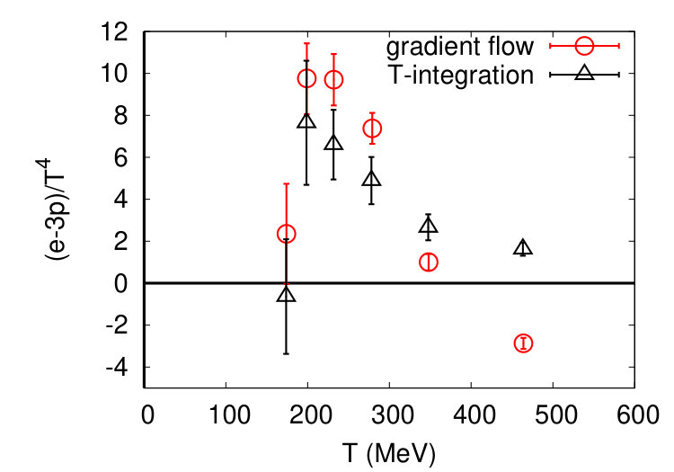 Figure 1
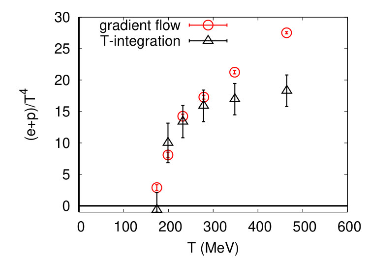 Figure 2
 Figure 3
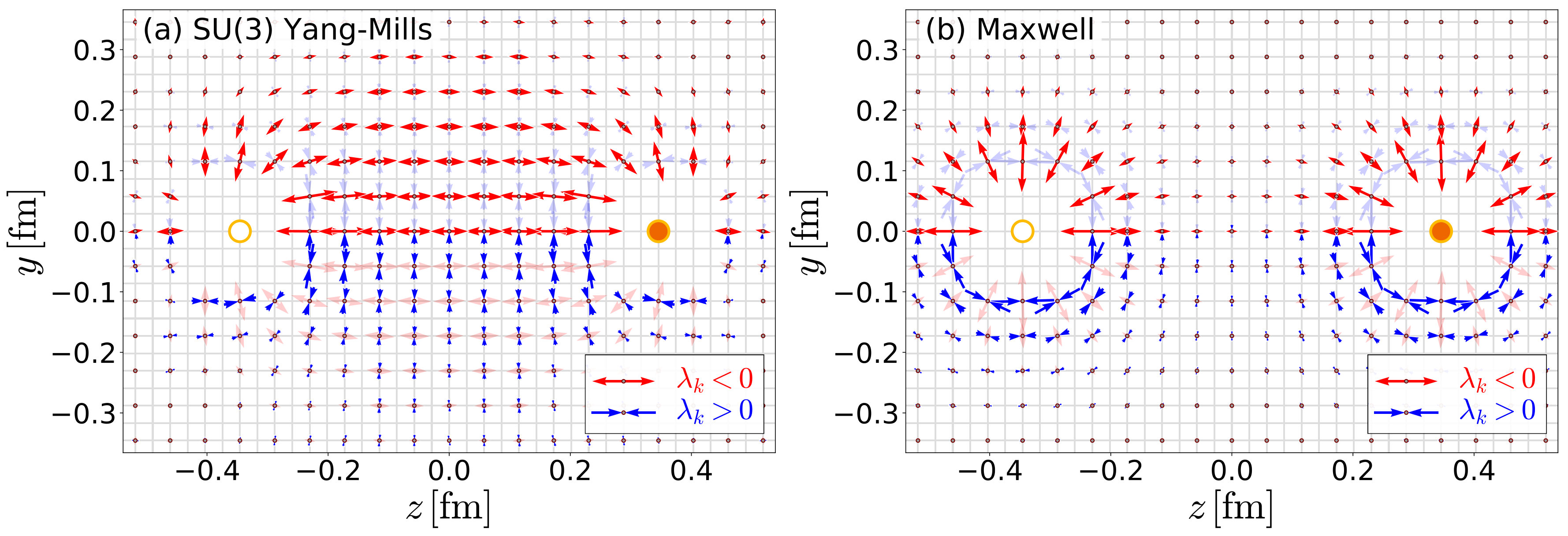 Figure 4
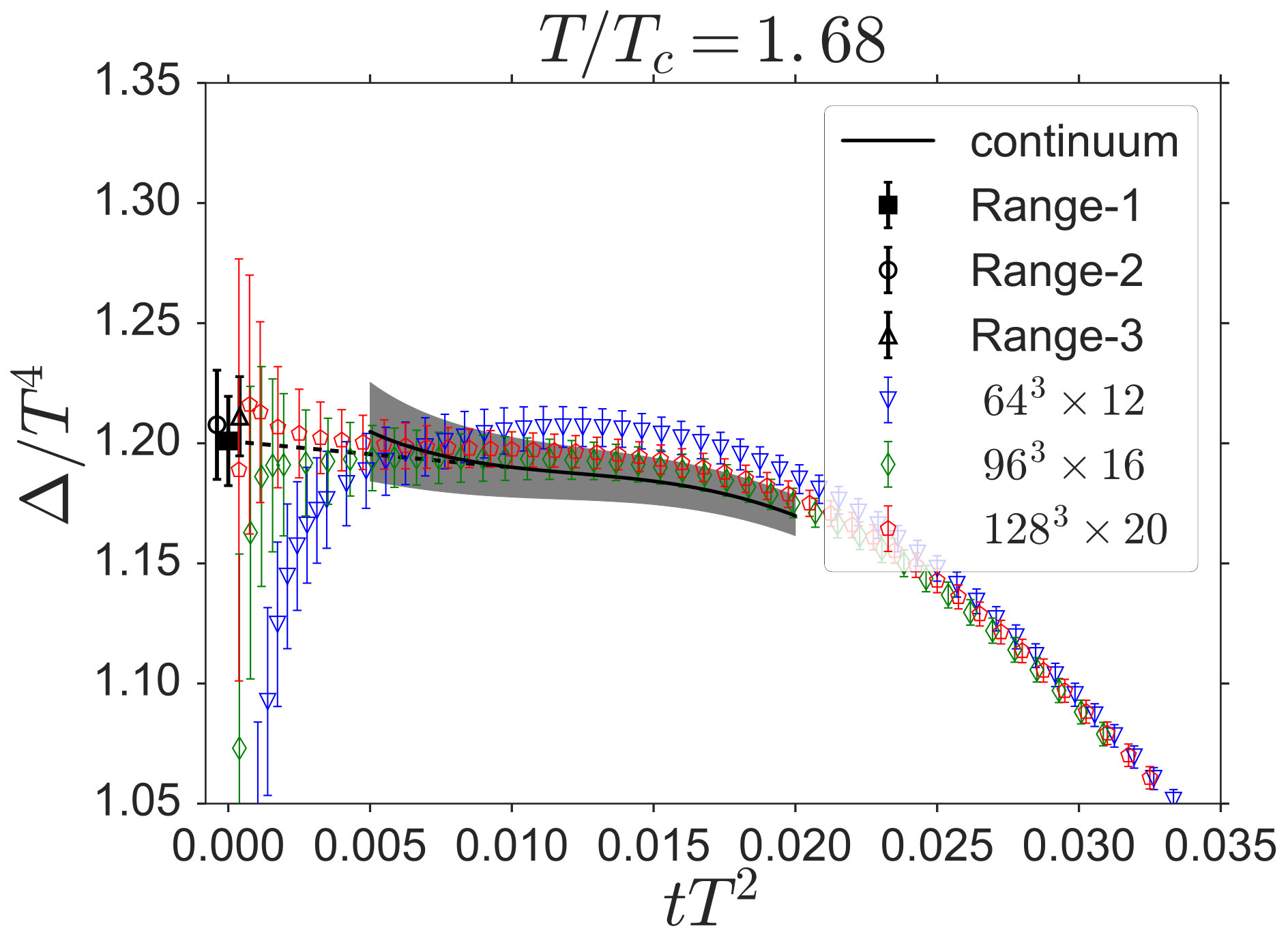 Figure 5
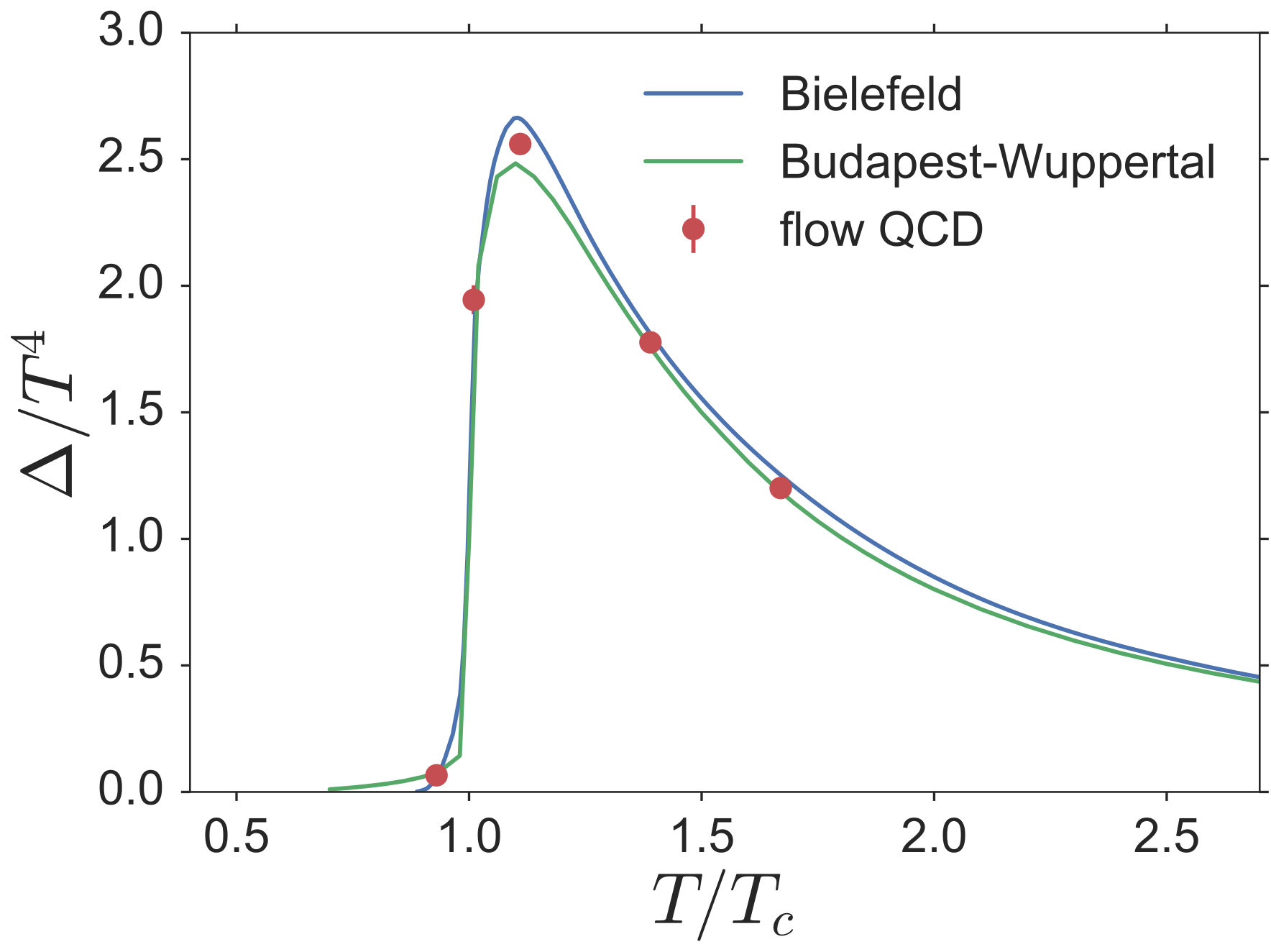 Figure 6
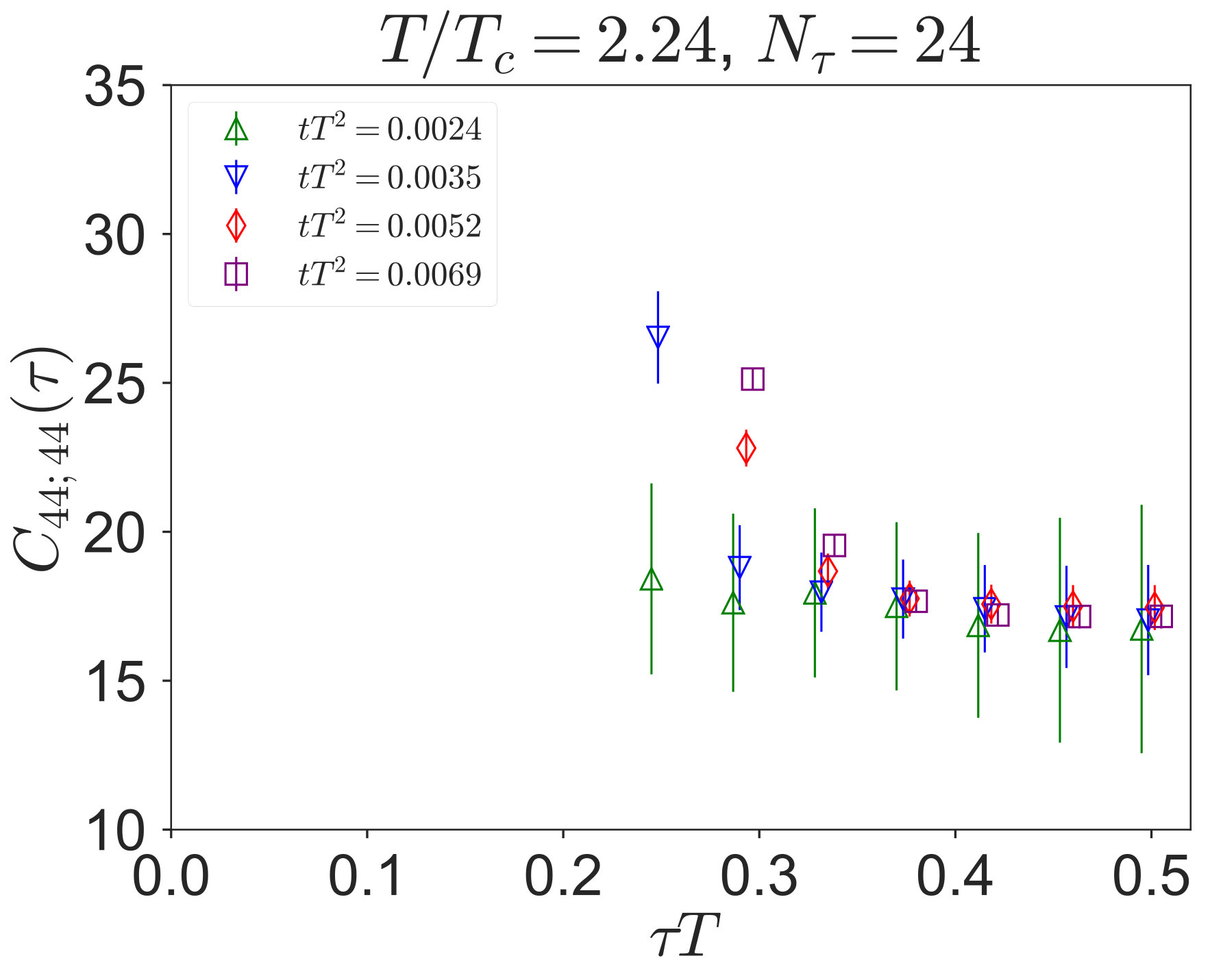 Figure 7
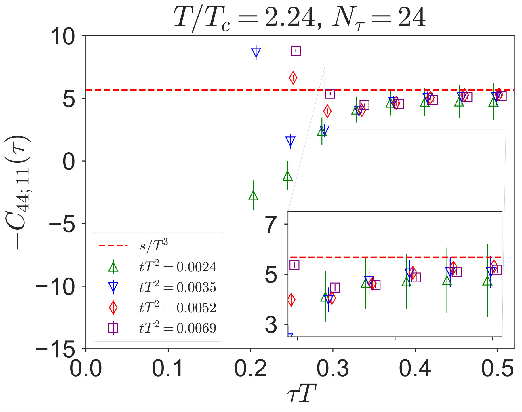 Figure 8
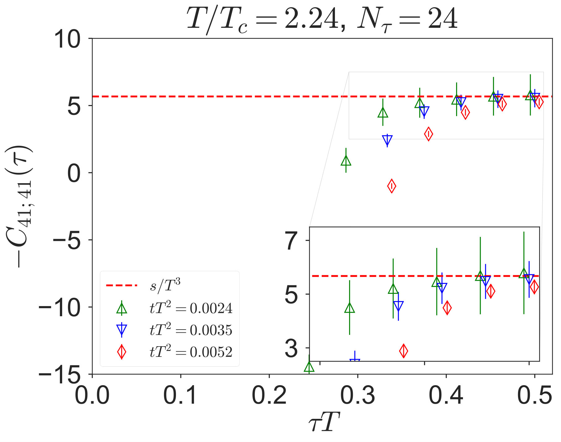 Figure 9
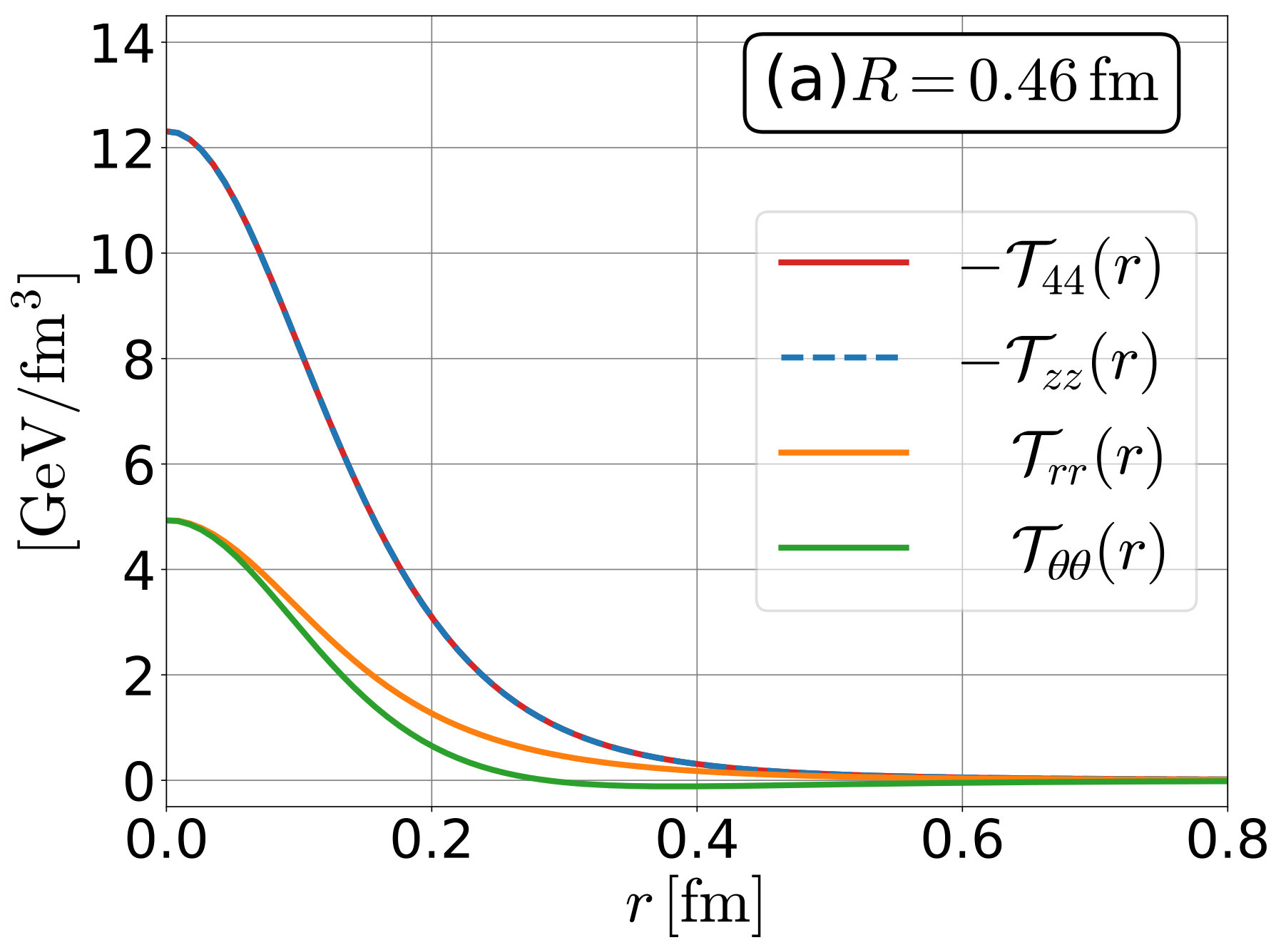 Figure 10
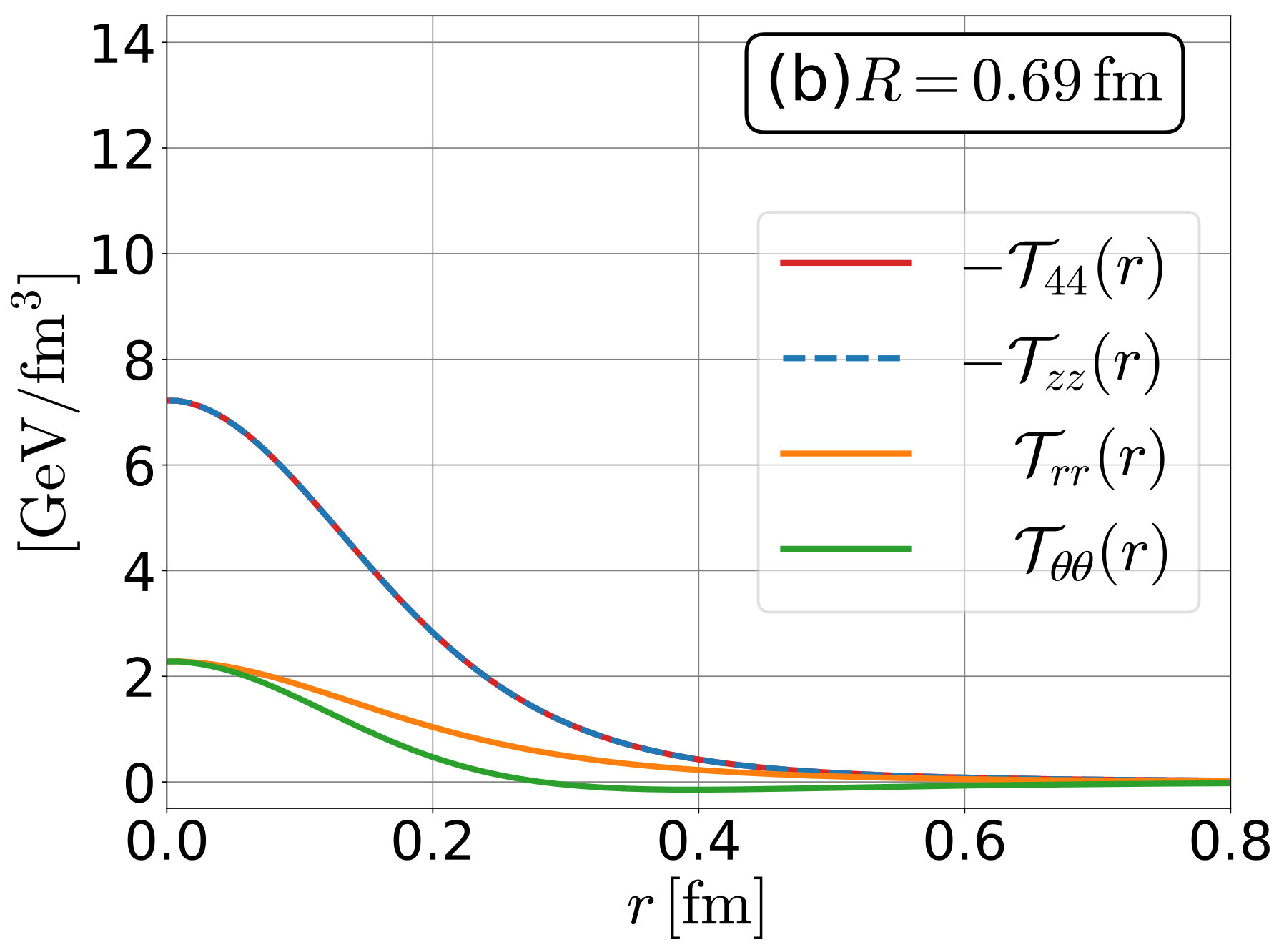 Figure 11
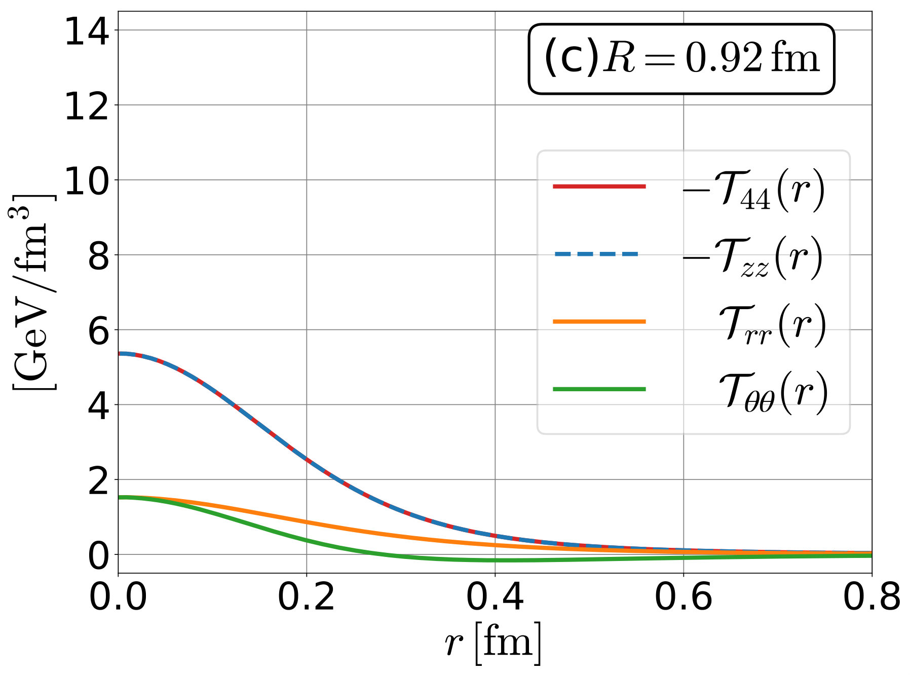 Figure 12
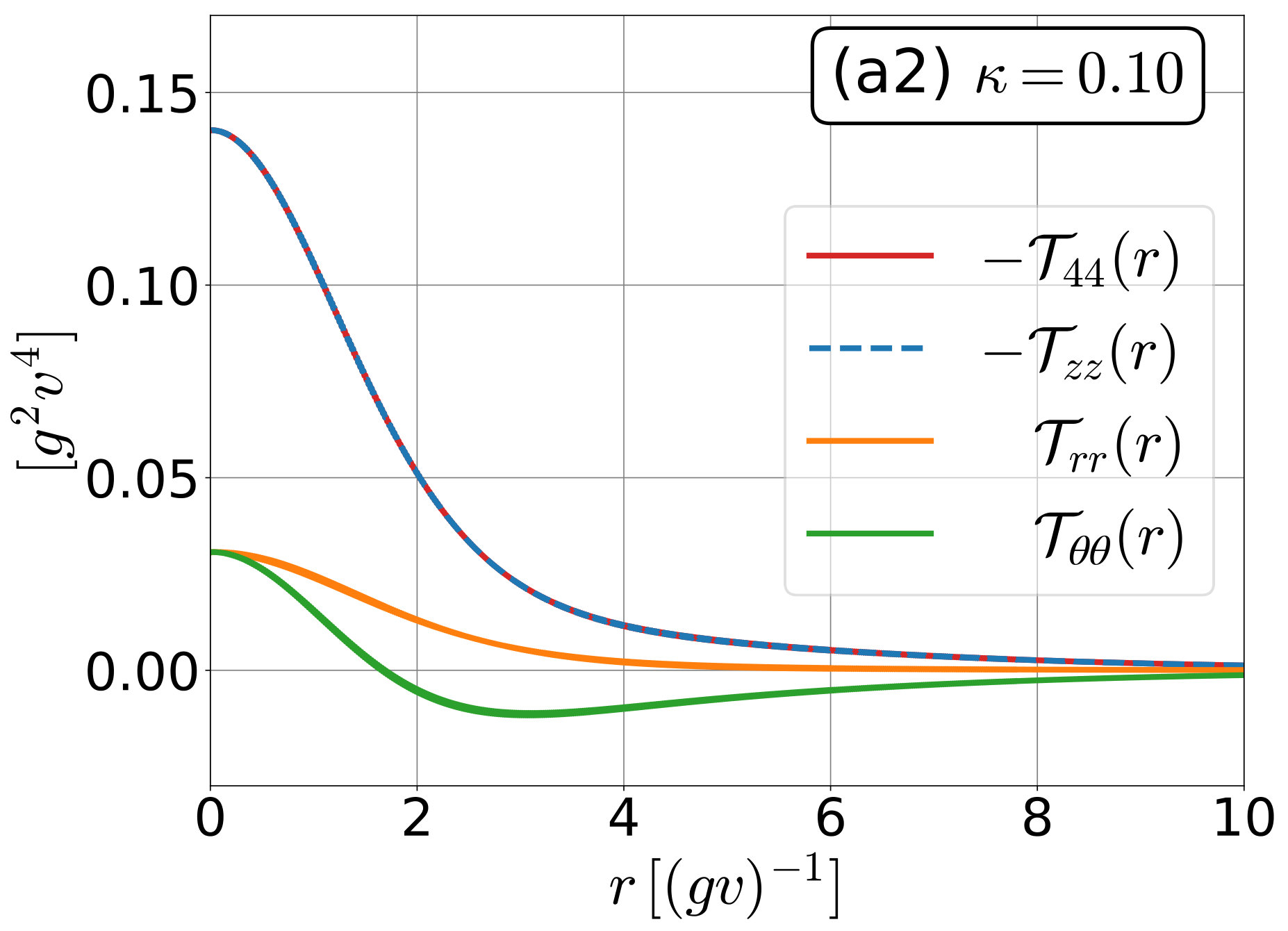 Figure 13
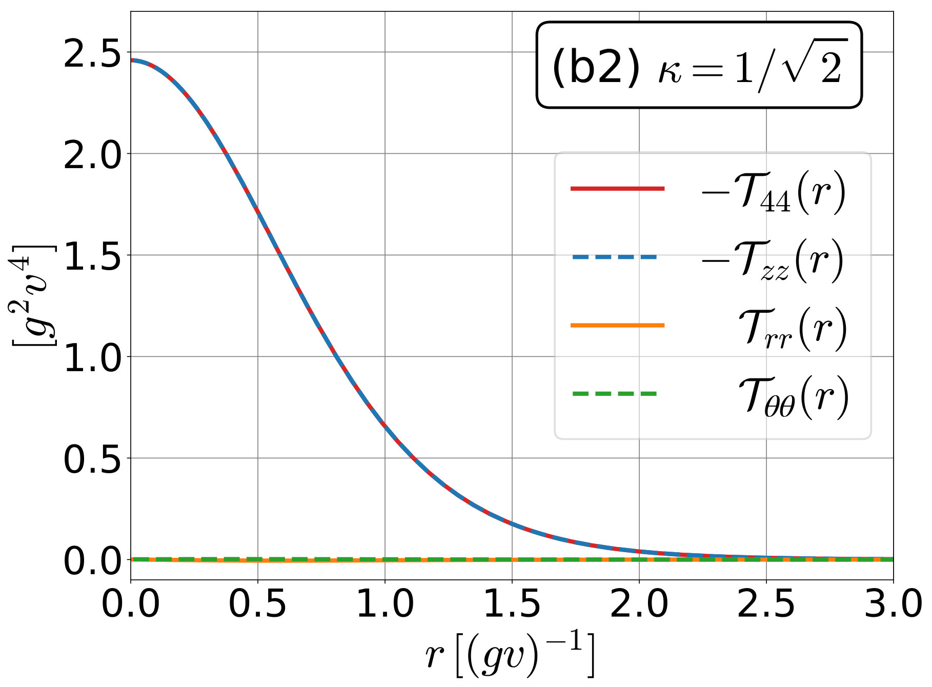 Figure 14
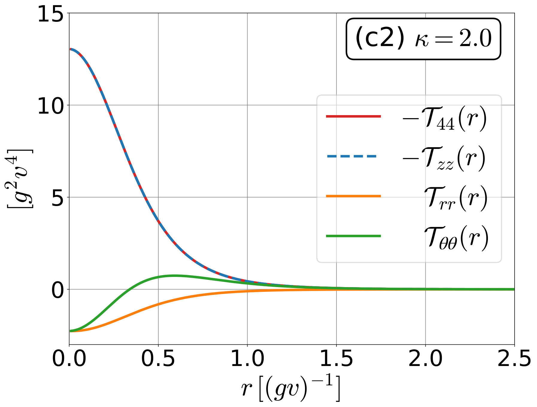 Figure 15
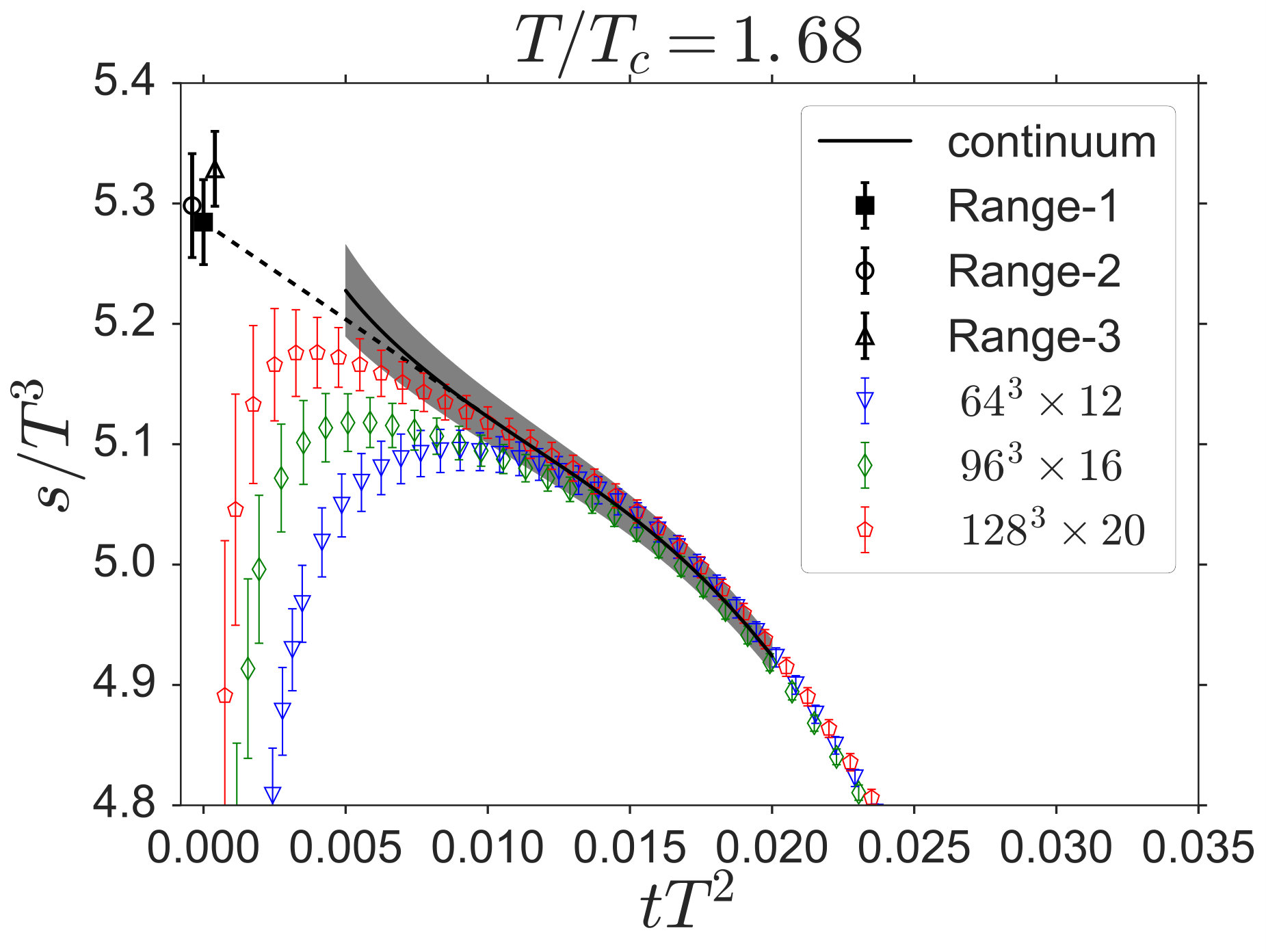 Figure 16
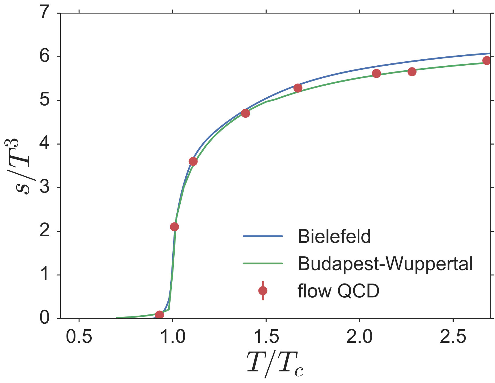 Figure 17
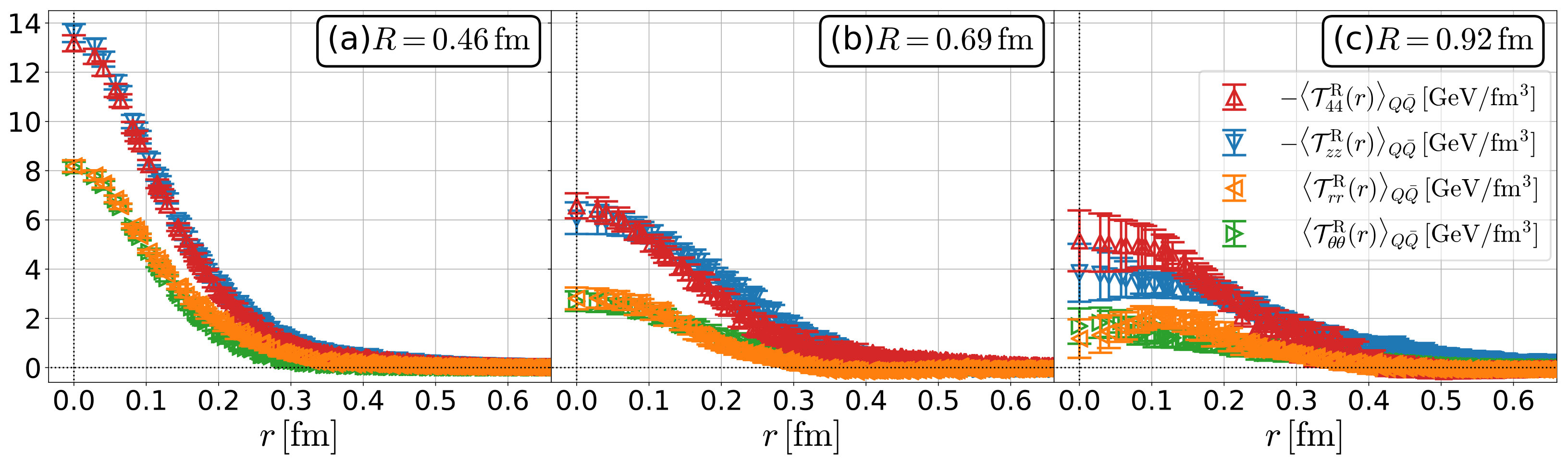 Figure 18
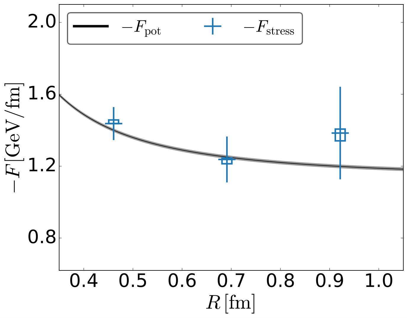 Figure 19
Peer Reviews
No public reviews on file for this paper yet. If you reviewed it on a platform where reviews are public (OpenReview, ICLR, NeurIPS, ICML), you can paste yours below so the community can read it here.
Videos
No videos yet. Explain this paper in a talk, walkthrough, or lecture? Add one.
J-PARC-TH-0157 Exploring non-abelian gauge theory with energy-momentum tensor; stress, thermodynamics and correlations
Department of Physics, Osaka University, Toyonaka, Osaka 560-0043, Japan
J-PARC Branch, KEK Theory Center, Institute of Particle and Nuclear Studies, KEK, 203-1, Shirakata, Tokai, Ibaraki 319-1106, Japan
Abstract:
We perform various lattice numerical analyses with the energy-momentum tensor (EMT) defined through the gradient flow. We explore the spatial distribution of the stress tensor in static quark-anti-quark systems and thermodynamic quantities at nonzero temperature, as well as the correlation functions of EMT. The stress tensor distribution is also studied in the Abelian-Higgs model, which is compared with the lattice result.
1 Introduction
The energy-momentum tensor (EMT)
[TABLE]
is one of the most fundamental observables in physics. It’s temporal and spatial components are related to important quantities in physics, i.e. energy density , momentum density , and the stress tensor , as
[TABLE]
Among these observables, the stress tensor is a particularly interesting quantity because it represents the distortion of the field which mediates the force between charges. The direct analysis of the stress tensor in various systems in QCD, such as static-quark systems and hadrons, will provide us with deeper understanding on these systems based on microscopic points of view in a gauge invariant manner. In a thermal system at nonzero temperature, is given by a diagonal matrix representing the pressure, which is a basic information on thermodynamics.
Recently, considerable developments have been made in numerical analyses of EMT in lattice gauge theory [1]. In particular, it was found [2] that the analysis of EMT on the lattice can be performed successfully with the use of the gradient flow [3, 4, 5]. Because EMT is a fundamental observable in physics, its analyses on the lattice will provide us with new insights into QCD and non-Abelian gauge theories.
In this proceeding, after introducing the EMT operator on the lattice constructed from the gradient flow in Sec. 2, we discuss recent applications of the EMT operator to the analysis of various quantities, thermodynamics (Sec. 3), EMT correlation functions (Sec. 4), and the stress distribution in the system (Sec. 5).
2 Energy-momentum tensor and gradient flow
Let us first see the construction of EMT using the gradient flow [2]. The gradient flow for the YM theory is a continuous transformation of the gauge field defined by the differential equation [3, 4, 5]
[TABLE]
with the Yang-Mills action composed of the field at nonzero flow time . The initial condition at is taken for the conventional gauge field; . The flow time , which controls the magnitude of transformation, has a dimension of inverse mass squared. At the tree level, Eq. (3) is written as
[TABLE]
Neglecting the gauge dependent term, Eq. (4) is the diffusion equation in four-dimensional space. Therefore, the gradient flow for positive acts as a cooling of the gauge field with smearing radius .
In the present study, we use the gradient flow to introduce the EMT operator using the small flow time expansion (SFTE) [5, 2]. The SFTE asserts that a composite operator composed of the field at is represented in terms of the operators in the original gauge theory as
[TABLE]
in the small limit, where on the right-hand side are renormalized operators in the original gauge theory at with the subscript denoting different operators.
In order to construct EMT using Eq. (5), we expand the following operators via the SFTE;
[TABLE]
The SFTEs of Eqs. (6) and (7) are given by
[TABLE]
where denotes vacuum expectation value and is the correctly renormalized EMT. Abbreviated are the contributions from the operators of dimension or higher, which are proportional to powers of because of dimensional reasons and suppressed for small .
Combining Eqs. (8) and (9), we obtain
[TABLE]
The coefficients and are calculated perturbatively up to one- and two-loop orders, respectively, in Ref. [2]111 The perturbative analyses of and are recently extended to one more higher order; see Refs. [10, 11]. . We use these coefficients in the following analysis.
The concept of the gradient flow and the construction of EMT via the SFTE can also be extended to full QCD with fermions [6, 7, 8, 9]. In this case, one needs five operators for the SFTE of EMT; in addition to Eqs. (6) and (7), there are three operators including fermions at dimension . The coefficients in the SFTE in this case is calculated in Ref. [7] (see also Ref. [10]).
From Eq. (10), one can obtain in the numerical simulation of lattice gauge theory by the following procedure:
Generate gauge configurations at with a standard algorithm. 2. 2.
Obtain the flowed gauge field for by numerically solving the flow equation (3). 3. 3.
Analyze and on the flowed field at each , and determine in Eq. (10). Then construct the expectation value or correlation functions of . 4. 4.
Carry out the double extrapolation to where is the lattice spacing.
In the last step for the double extrapolation, the analysis has to be performed in the parameter range satisfying , where is an infrared cutoff scale such as , or the shortest length relevant for the problem such as for temperature and distances between operators. The condition is necessary to suppress the finite correction which diverges for .
3 Thermodynamics
Now let us apply the EMT operator defined in the previous section to the analysis of thermodynamic quantities in SU(3) YM theory [12, 13]. In the following, we consider and the entropy density given by linear combinations of the energy density and pressure .
In Fig. 1, we plot
[TABLE]
as functions of at obtained on the lattices with three different lattice spacings [13]. To take the double extrapolation from these results, we first carry out the continuum extrapolation for each . The result of this extrapolation is plotted by the black line with errors shown by the shaded region. We then take the limit using this continuum extrapolated result with three different fitting ranges of ; Range-1: , Range-2: , Range-3: . The extrapolated values with these ranges are shown in the figure around . Their difference is taken into account in the systematic error in the final result.
The dependence of thermodynamic quantities and in SU(3) YM theory obtained by this step is shown in Fig. 2 by the red circles [13]. In the figure, the results obtained by the conventional integral method [14, 15] are also plotted. It is remarkable that the values of and obtained by the completely different methods agree well with each other. This agreement suggests that EMT is successfully analyzed in the lattice simulation with the gradient flow by the procedure introduced in the previous section.
Recently, novel methods to measure thermodynamics in lattice gauge theory have been proposed [16, 17, 18, 19] besides the integral and gradient flow methods, and they are applied to SU(3) YM theory. As summarized in Refs. [19, 11], all these results agree well with each other, but there exists small but statistically significant discrepancy above but near . Understanding the origin of this difference is an important future study in the accurate measurement of thermodynamics.
The analysis of thermodynamics by the gradient flow method can be applied to full QCD simulation with fermions [7, 8]. In Fig. 3, we show the dependences of and in (2+1)-flavor QCD obtained by the gradient flow method by the red circles, together with the results of the integral method obtained on the same gauge configurations [8]. The mass of quarks is slightly heavy in this simulation; . Since the numerical simulation in this study is performed only for a single lattice spacing, the extrapolation is taken without the continuum extrapolation to obtain the final result in Fig. 3. Various extrapolating functions are adopted to take the extrapolation from numerical results at . Fig. 3 shows that the two results agree well with each other except for the high temperature region at which the extrapolation is unstable.
4 EMT correlation functions
Next, we apply the EMT operator Eq. (10) to the analysis of the imaginary-time correlation function of EMT [20]
[TABLE]
The EMT correlation function at nonzero temperature contains various important information. For example, the spatial components are related to transport coefficient through Kubo formula [21]. However, is known to be extremely noisy in lattice simulations [21].
Here, as a first analysis of with the gradient flow method, we focus on the channels including conserved quantities, i.e. , , and . Because of the energy and momentum conservation, these correlators do not have a dependence for . Moreover, from thermodynamic relations they are given by
[TABLE]
for where is the specific heat per unit volume.
Shown in Fig. 4 are the correlation functions , , and in SU(3) YM theory calculated on the lattice with and [20]. The results are shown for several values of the flow time . The figure shows that there exists a independent plateau for which is consistent with the conservation of energy and momentum. The disappearance of the plateau at comes from the over-smearing due to the gradient flow. To check the second equation in Eq. (13), in the middle and right panels of Fig. 4 the value of is shown by the red-dashed line. The panels show that and satisfy Eq. (13). More detailed verification of Eq. (13) with the double extrapolation , as well as the analysis of with the use of the first equation in Eq. (12), is carried out in Ref. [20].
From these results, one finds that the EMT operator Eq. (10) is successfully applied to the analysis of the EMT correlator Eq. (12). Therefore, it is an interesting subject to apply this method to the analysis of the spatial channels of Eq. (12) which are relevant for the transport coefficient. Recently, the analysis of these channels with the conventional EMT operator in SU(3) YM theory has been updated in Refs. [22, 23]. Because these studies use multi-level algorithm, however, it is difficult to extend the analysis to full QCD. The analysis of Eq. (12) in full QCD with the gradient flow method is reported in Ref. [24].
5 Stress tensor distribution around
Now we consider the spatial component of EMT which is related to the stress tensor as in Eq. (2). In this section, we apply the EMT operator Eq. (10) to the analysis of the stress-tensor distribution in static quark–anti-quark () systems in SU(3) YM theory [25] in which the YM field strength is squeezed into a quasi-one-dimensional flux-tube structure [26]. In the previous studies, the spatial structure of the flux tube has been investigated using the action density and the color electric field. Compared with these observables, has clear physical meanings; the stress tensor represents the local interaction mediated by the distortion of the YM field. Moreover, the stress tensor enables us to study this system in a manifestly gauge invariant manner.
To prepare a static system on the lattice, we use the standard Wilson loop with static color charges at and in the temporal interval . Then the expectation value of around the is obtained by
[TABLE]
where is to pick up the ground state of . In actual numerical simulations, we use the APE smearing for each spatial link to enhance the coupling of to the ground state with fixed . We also adopt the standard multi-hit procedure by replacing each temporal link by its mean-field value to reduce the statistical noise. The measurements of for different values of are made at the mid temporal plane , while is defined at .
Before taking the double limit , we illustrate a qualitative feature of the distribution of around at fixed and with . In Fig. 5 (a) [25], we show the two eigenvectors of the stress tensor defined by
[TABLE]
along with the principal axes of the local stress. The eigenvector with negative (positive) eigenvalue is denoted by the red outward (blue inward) arrow with its length proportional to :
[TABLE]
Neighboring volume elements are pushing (pulling) with each other along the direction of blue (red) arrow. The spatial regions near and , which would suffer from over-smearing, are excluded in the figure. Spatial structure of the flux tube is clearly revealed through the stress tensor in Fig. 5 (a) in a gauge invariant way. This is in contrast to the same plot of the principal axes of for opposite charges in classical electrodynamics shown in Fig. 5 (b).
We note that the red arrows in Fig. 5 are naturally interpreted as the direction of the line of field. In this sense, Fig. 5 (a) is a first gauge invariant illustration of the line of the color electric field in YM theory.
Next, we focus on the mid-plane between the with and extract the stress-tensor distribution by taking the double extrapolation [25]. On the mid-plane, it is convenient to use the cylindrical coordinate system with and . One can show that the EMT on the mid-plane is diagonalized in this coordinate as
[TABLE]
Shown in Fig. 6 is the dependence of the resulting EMT, i.e. the stress tensor and the energy density with three distances fm [25]. From the figure, one finds several notable features. First, approximate degeneracy as well as is found for a wide range of and . Second, the nonzero value of the trace of EMT is observed, which suggests the partial restoration of the scale symmetry broken in the YM vacuum. Finally, the radius of the flux tube, typically about fm, seems to become wider with increasing .
Next, we consider a non-trivial consistency check for the uniqueness of the force [25]. The force acting on the charge located at can be obtained by two different manners; (i) through the potential as
[TABLE]
and (ii) from the surface integral of the stress-tensor surrounding the charge,
[TABLE]
For , we use the numerical data of obtained from the Wilson loop at fm. For , we take the mid-plane for the surface integral: . In Fig. 7, and thus obtained are shown by the solid line and the horizontal bars, respectively [25]. The figure shows the agreement between the two quantities within the errors, which is a first numerical evidence that the “action-at-a-distance” force can be described by the local properties of the stress tensor in YM theory.
6 Analysis of system in Abelian-Higgs model
Finally, let us investigate the behavior of in Fig. 6 in more detail especially focusing on the approximate degeneracy and separation of each channel, [27].
First, from the momentum conservation, , one can show that the EMT in the cylindrical coordinates Eq. (17) satisfies Then, by further assuming that the flux tube is sufficiently long so that it has a translational invariance along the direction, the derivative vanishes and one obtains,
[TABLE]
From this differential equation it is concluded that and do not degenerate except for the case . Moreover, by integrating out both sides of Eq. (20) by and using the boundary conditions for and , one obtains
[TABLE]
which means that must change the sign at least once. Such behaviors of and , however, are not observed in Fig. 6 even at the largest distance. It is therefore suggested that the finite-length effect of the flux tube is not negligible even at fm in SU(3) YM theory.
Next, in order to get ideas on physics behind the results in Fig. 6 we study the EMT distribution in a specific model. For this purpose, here we employ the Abelian-Higgs (AH) model
[TABLE]
which is the relativistic extension of the Ginzburg-Landau model, with the field strength and the covariant derivative . The AH model has classical solutions with a static magnetic vortex. When this model is viewed as an effective model of QCD according to the dual-superconductor picture [28], the vortex solution is considered as an analogue of the flux tube in YM theory. In the following, we thus study the EMT distribution around the classical vortex solution of Eq. (22) with the winding number . [27]
We first consider the EMT distribution around an infinitely-long and straight vortex. In Fig. 8, we show the EMT in cylindrical coordinates on the cross section of the vortex as a function of radius . Three panels show the results for different values of the Ginzburg-Landau parameter . From the figure, one finds that and have a clear separation except with at which . This separation is a model independent feature anticipated from the momentum conservation Eq. (20).
Next, we investigate the vortex with finite length . In AH model, the magnetic vortex with boundaries is obtained by putting two magnetic monopoles with a unit charge but opposite signs [29]. Shown in Fig. 9 are examples of the EMT distribution on the mid-plane between two monopoles [27]. The physical dimension in the figure is introduced by setting the energy density per unit length of the infinitely-long vortex to be the string tension obtained on the lattice. The model parameters are chosen so that the values of at are consistent with the lattice result in Fig. 6 after setting the length to be equivalent with the distance in the lattice simulations. The figure shows that the difference between and becomes small compared to Fig. 8. However, and still have a separation which would be inconsistent with Fig. 6. It is thus suggested that the degeneracy of these channels is a unique feature of the flux tube in SU(3) YM theory which cannot be reproduced by AH model.
7 Summary and outlook
In this proceeding, we reviewed recent attempts to perform the measurement of EMT on the lattice with the gradient flow and its applications to thermodynamics, correlations, and the stress-tensor distribution inside the flux tube. All these results show that EMT is successfully analyzed in lattice simulations with a reasonable statistics.
Now that the analysis of the EMT on the lattice is established, there are many further applications, as EMT is one of the most fundamental observables in physics. For example, it is quite interesting to extend the study of the flux tube to nonzero temperature, multi-quark systems, and excited states. It is also an interesting future study to analyze the EMT distribution inside hadrons [30, 31, 32] using the gradient flow method.
This work was supported by JSPS KAKENHI No. JP17K05442. Numerical simulation was carried out on IBM System Blue Gene Solution at KEK under its Large-Scale Simulation Program, Reedbush-U at the University of Tokyo, and OCTOPUS at Osaka University.
The reference list from the paper itself. Each links out to its DOI / PubMed record.
- 1[1] H. Suzuki, Po S LATTICE 2016 , 002 (2017) [ar Xiv:1612.00210 [hep-lat]], and references therein.
- 2[2] H. Suzuki, PTEP 2013 , no. 8, 083B 03 (2013) [Erratum: PTEP 2015 , no. 7, 079201 (2015)] [ar Xiv:1304.0533 [hep-lat]].
- 3[3] M. Lüscher, JHEP 1008 , 071 (2010) [ar Xiv:1006.4518 [hep-lat]].
- 4[4] R. Narayanan and H. Neuberger, JHEP 0603 , 064 (2006) [hep-th/0601210].
- 5[5] M. Lüscher and P. Weisz, JHEP 1102 , 051 (2011) [ar Xiv:1101.0963 [hep-th]].
- 6[6] M. Luscher, JHEP 1304 , 123 (2013) [ar Xiv:1302.5246 [hep-lat]].
- 7[7] H. Makino and H. Suzuki, PTEP 2014 , no. 6, 063B 02 (2014) [Erratum: PTEP 2015 , no. 7, 079202 (2015)] [ar Xiv:1403.4772 [hep-lat]].
- 8[8] Y. Taniguchi, S. Ejiri, R. Iwami, K. Kanaya, M. Kitazawa, H. Suzuki, T. Umeda, and N. Wakabayashi, Phys. Rev. D 96 , 014509 (2017) [ar Xiv:1609.01417 [hep-lat]].