Approximation Algorithms for the A Priori TravelingRepairman
Inge Li G{\o}rtz, Viswanath Nagarajan, Fatemeh Navidi

TL;DR
This paper introduces the first constant-factor approximation algorithm for the a priori traveling repairman problem with non-uniform probabilities, advancing the understanding of stochastic routing problems.
Contribution
It provides the first constant-factor approximation algorithm for the a priori TRP with non-uniform probabilities, extending previous results limited to uniform probabilities.
Findings
First constant-factor approximation for non-uniform probabilities in a priori TRP.
Algorithm effectively minimizes expected arrival times in stochastic routing.
Advances theoretical understanding of stochastic traveling repairman problems.
Abstract
We consider the a priori traveling repairman problem, which is a stochastic version of the classic traveling repairman problem (also called the traveling deliveryman or minimum latency problem). Given a metric with a root , the traveling repairman problem (TRP) involves finding a tour originating from that minimizes the sum of arrival-times at all vertices. In its a priori version, we are also given independent probabilities of each vertex being active. We want to find a master tour originating from and visiting all vertices. The objective is to minimize the expected sum of arrival-times at all active vertices, when is shortcut over the inactive vertices. We obtain the first constant-factor approximation algorithm for a priori TRP under non-uniform probabilities. Previously, such a result was only known for uniform probabilities.
Click any figure to enlarge with its caption.
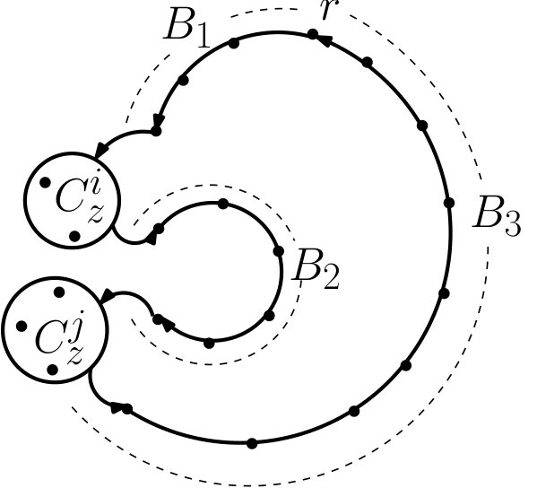 Figure 1
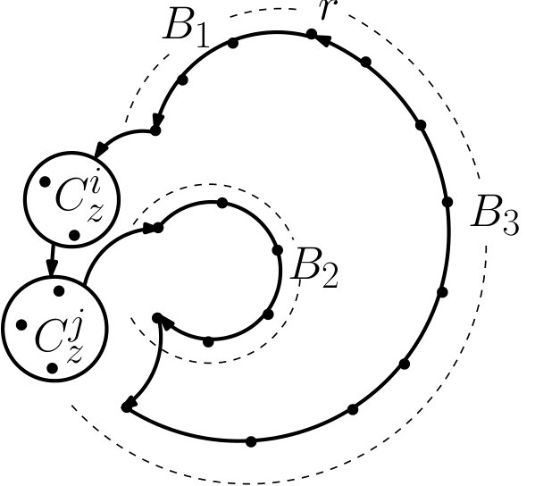 Figure 2
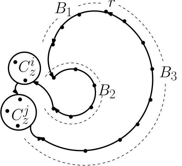 Figure 3
Peer Reviews
No public reviews on file for this paper yet. If you reviewed it on a platform where reviews are public (OpenReview, ICLR, NeurIPS, ICML), you can paste yours below so the community can read it here.
Videos
No videos yet. Explain this paper in a talk, walkthrough, or lecture? Add one.
Taxonomy
TopicsOptimization and Search Problems · Complexity and Algorithms in Graphs · Machine Learning and Algorithms
Approximation Algorithms for the A Priori Traveling Repairman
Inge Li Gørtz [email protected] Technical University of Denmark, DTU Compute, Denmark
Viswanath Nagarajan [email protected] University of Michigan, Ann Arbor, MI, USA
Fatemeh Navidi [email protected] University of Michigan, Ann Arbor, MI, USA
Abstract
We consider the a priori traveling repairman problem, which is a stochastic version of the classic traveling repairman problem (also called the traveling deliveryman or minimum latency problem). Given a metric with a root , the traveling repairman problem (TRP) involves finding a tour originating from that minimizes the sum of arrival-times at all vertices. In its a priori version, we are also given independent probabilities of each vertex being active. We want to find a master tour originating from and visiting all vertices. The objective is to minimize the expected sum of arrival-times at all active vertices, when is shortcut over the inactive vertices. We obtain the first constant-factor approximation algorithm for a priori TRP under non-uniform probabilities. Previously, such a result was only known for uniform probabilities.
Keywords Traveling Repairman Problem, A Priori Optimization, Approximation Algorithms
1 Introduction
Traditional optimization models assume full information on the instances being solved, which is unrealistic in many situations. In order to remedy this limitation, there has been significant work in the area of optimization under uncertainty, which deals with various ways to model uncertain input. Stochastic optimization is a widely used approach, where one models the input probabilistically.
A priori optimization ([5]) is an elegant model for stochastic combinatorial optimization, that is particularly useful when one needs to repeatedly solve instances of the same optimization problem. The basic idea here is to reduce the computational overhead of solving repeated problem instances by performing suitable pre-processing using distributional information. More specifically, in an a priori optimization problem, one is given a probability distribution over inputs and the goal is to find a “master solution” . Then, after observing the random input (drawn from the distribution ), the master solution is modified using a simple rule to obtain a solution for that particular input. The objective is to minimize the expected value of the master solution. For a problem with objective function , we are interested in:
[TABLE]
This paper studies the a priori traveling repairman problem. The traveling repairman problem (TRP) is a fundamental vehicle routing problem that involves computing a tour originating from a depot/root that minimizes the sum of latencies (i.e. the distance from the root on this tour) at all vertices. The TRP is also known as the traveling deliveryman or minimum latency problem, and has been studied extensively, see e.g. [16], [10], [11]. In the a priori TRP, the master solution is a tour visiting all vertices, and for any random input (i.e. subset of vertices), the solution is simply obtained by visiting the vertices of in the order given by .
An a priori solution is advantageous in settings when we repeatedly solve instances of the TRP that are drawn from a common distribution. For example, we may need to solve one TRP instance on each day of operations, where the distribution over instances is estimated from historical data. Using an a priori solution saves on computation time as we do not have to solve each instance from scratch. Moreover, for vehicle routing problems (VRPs) there are also practical advantages to have a pre-planned master tour, e.g. drivers have familiarity with the route followed each day. See [17], [7], and [9] for more discussion on the benefits of a pre-planned VRP solution.
1.1 Problem Definition.
The traveling repairman problem (TRP) is defined on a finite metric where is a vertex set and is a distance function. We assume that the distances are symmetric and satisfy triangle inequality. There is also a designated root vertex . The goal is to find a tour originating from that visits all vertices. The latency of any vertex in tour is the length of the path from to along . The objective in TRP is to minimize the sum of latencies of all vertices.
In the a priori TRP, in addition to the above input we are also given activation probabilities at all vertices; we use to denote this distribution. In this paper, as in most prior works on a priori optimization, we assume that the input distribution is independent accross vertices. So the active subset contains each vertex independently with probability . A solution to a priori TRP is a master tour originating from and visiting all vertices. Given an active subset , we restrict tour to vertices in (by shortcutting over ) to obtain tour , again originating from . For each , we use to denote the latency of in tour . We also use for the total latency under active subset . The objective is to minimize
[TABLE]
1.2 Results.
Our main result in this note is the first constant-factor approximation for the a priori TRP.
Theorem 1.1**.**
There is a constant-factor approximation algorithm for the a priori traveling repairman problem under independent probabilities.
Previously, [22] obtained such a result under the restriction that all activation probabilities are identical, and posed the general case of non-uniform probabilities as an open question– which we resolve. Our result adds to the small list of a priori VRPs with provable worst-case guarantees: traveling salesman, capacitated vehicle routing and traveling repairman.
In fact, we obtain Theorem 1.1 by a generic reduction of a priori TRP from non-uniform to uniform probabilities, formalized below.
Theorem 1.2**.**
There is a -factor approximation algorithm for the a priori traveling repairman problem under independent probabilities, where denotes the best approximation ratio for the problem under uniform probabilities.
Clearly, Theorem 1.1 follows by combining Theorem 1.2 with the -approximation algorithm for a priori TRP under uniform probabilities by [22]. As the constant factor in [22] for uniform probabilities is quite large, there is the possibility of improving it using a different algorithm: Theorem 1.2 would be applicable to any such future improvement and yield a corresponding improved result for non-uniform probabilities.
1.3 Related Work.
The a priori optimization model was introduced in [15] and [3], see also the survey by [5]. These papers considered the setting where the metric is itself random and carried out asymptotic analysis (as the number of vertices grows large). They obtained such results for the minimum spanning tree, traveling salesman, capacitated vehicle routing and traveling salesman facility location problems.
Approximation algorithms for a priori optimization are more recent: these can handle arbitrary problem instances. Such results are known for the traveling salesman problem (TSP), capacitated VRP and traveling repairman (TRP). We briefly discuss them below.
The a priori TSP has been extensively studied. In particular, there is a randomized -approximation algorithm for independent probabilities by [19]. The same paper also gave a deterministic -approximation algorithm; the constant was later improved to in [23]. These algorithms were based on a random-sampling approach ([13, 24]) that was previously used in other network design problems. For arbitrary (black-box) distributions, [18] gave a randomized -approximation algorithm which actually does not even need any knowledge on the distribution. Later, [12] proved an lower bound on the approximation ratio of any deterministic algorithm for a priori TSP under arbitrary distributions.
The capacitated VRP with stochastic demands ([4]) is another well-studied a priori optimization problem. Here, we have a vehicle with limited capacity at the root that needs to satisfy demands at various vertices. The demand at each vertex is an independent random variable with a known distribution. A master solution to this problem is a tour that visits every vertex; after demands are observed, the vehicle visits vertices in the same order as while performing additional refill-trips to the root whenever it runs out of items. The objective is to minimize the total length of the tour. A -approximation algorithm for this problem in the case of identical demand distributions was given in [4]. Later, [14] obtained a randomized -approximation algorithm for this problem under non-identical distributions.
The a priori TRP was recently studied in [22], where a constant-factor approximation algorithm was obtained for the case of uniform independent probabilities. They left open the problem under non-uniform probabilities: Theorem 1.2 resolves this positively. The algorithm in [22] was based on many ideas from the deterministic TRP, but it needed stochastic counterparts of various properties. As noted in [22], their proof relied heavily on the probabilities being uniform and it was unclear how to handle non-uniform probabilities.
We note that the deterministic traveling repairman problem (TRP) has been studied extensively, both in exact algorithms ([16, 10, 25]) and approximation algorithms ([6], [11], [2], [8]). It was shown to be NP-hard even on weighted trees by [20], and a polynomial time approximation scheme (PTAS) on such metrics was given by [21]. On general metrics, the best approximation ratio known is due to [8]; it is also known that one cannot obtain a PTAS.
2 A Priori TRP with Non-Uniform Distribution
Consider an instance of a priori TRP on metric with probabilities . We show how to “reduce” this instance to one with uniform probabilities, which would prove Theorem 1.2. Our approach is natural: we replace each vertex with a group of co-located vertices, where each new vertex is active with a uniform probability . Let denote the new instance and the new metric. Intuitively, when is chosen much smaller than the s and , the scaled uniform instance should behave similar to . However, proving such a result formally requires significant technical work. For example, the master tour found by an algorithm for the scaled (uniform) instance might not visit all the co-located copies consecutively. We define a consecutive master tour for as one that visits all co-located vertices consecutively. Then, we show an approximate equivalence between (i) master tours in and (ii) consecutive master tours in . This relies on the independence across vertices and the correspondence between the events “vertex is active in ” and “at least one vertex of is active in ”. This is formalized in Section 2.2. Then, we show in Section 2.4 that any master tour for instance can be modified to a “consecutive” master tour with the same or better overall expected latency. Finally, in order to maintain a polynomial-size instance (this is reflected in the choice of ), we need to take care of vertices with very small probability separately. In Section 2.3 we show that the overall effect of the small-probability vertices is tiny if they are visited in non-decreasing order of distances at the end of our master tour.
Algorithm 1 describes the reduction formally. In Step 6, Algorithm 1 relies on a procedure MakeConsecutive that modifies tour such that it visits all copies of the same node consecutively. We will prove Theorem 1.2 by analyzing this algorithm.
2.1 Overview of Analysis.
We first assume that the master tour on instance already visits copies of each vertex consecutively: so there is no need for Step 6. We split this proof into two parts corresponding to the -vertices (normal probabilities) and -vertices (low probabilities). The analysis for -vertices (Section 2.2) is the main part, where we show that the optimal values of and are within a constant factor of each other. In Lemma 2.3 we show that a constant-factor perturbation in probabilities of will only change the cost of any solution (including the optimal) by a constant factor. Then we prove (in Lemma 2.4) that the optimal value of instance is within a constant factor of the optimal value of : although has many more vertices than , the proof exploits the fact that the expected number of active vertices is roughly the same as . Lemma 2.5 proves the other direction for the cost of our algorithm, i.e. the cost of Algorithm 1 for is at most that of the consecutive master tour for . To handle the -vertices, we use a simple expected distance lower-bound to show (in Section 2.3) that visiting at the end of our tour only adds a small factor to the overall expected cost.
Note that we assumed above that the master tour visits copies of each vertex consecutively. It is possible that the algorithm for uniform a priori TRP in [22] already has this property, in which case the analysis outlined above suffices. However, by providing an explicit subroutine (MakeConsecutive) that ensures this consecutive property, our approach can be combined with any algorithm for uniform a priori TRP. The details of the MakeConsecutive procedure and its analysis appear in Section 2.4.
2.2 Analysis for vertices in X.
Here we analyze the steps of the algorithm that deal with vertices in , i.e. with probability at least . In order to reduce notation, we will assume here that which is the entire vertex set. Recall that . Also define , and for each . We will refer to the instances on metric with probabilities , and as , and respectively. Note that the original instance is . For simplicity we use and to refer to the vector of probabilities for each corresponding distribution.
Lemma 2.1**.**
For any , we have .
Proof.
Note that for every real number we have : using and raising both sides to the power of we obtain . Now we have:
[TABLE]
The second inequality uses and the last one uses for any with . Now, to prove the other inequality we consider the bionomial expansion of and cut it off for the powers greater than 1. So we have:
[TABLE]
Combined with the fact that , we obtain . ∎
Lemma 2.2**.**
Let be any master tour on . Consider two probability distributions given by and such that for each . Then the expected latency of under is at most that under .
Proof.
Let function denote the expected latency of as a function of vertex probabilities . We will show that all partial derivatives of are non-negative. This would imply the lemma.
We can express as a multilinear polynomial
[TABLE]
Recall that is the total latency of vertices in active set in the shortcut tour . So the partial derivative is:
[TABLE]
For any , it follows by triangle inequality that . This shows that each term in the above summation is non-negative and so . ∎
Lemma 2.3**.**
Let be any master tour on . Consider two probability distributions given by and and some constant such that for each . Then the expected latency of under is at least times that under .
Proof.
Let function denote the expected latency of under probabilities . For and as in the lemma, we will show . To this end, we now view as the expected sum of terms corresponding to all possible edges used in the shortcut tour (where is the active set). Renumber the vertices as in the order of appearance in ; so the root is numbered . For any let denote the indicator random variable for (ordered) edge being used in the shortcut tour . For any , let denote the number of active vertices among . Then, the total latency of tour is
[TABLE]
Under probabilities , for any we have which corresponds to the event that and are active but all vertices between and are inactive. Moreover, using the independence across vertices. So we can write:
[TABLE]
Note that for any , using the fact that we have:
[TABLE]
This implies as desired. ∎
Lemma 2.4**.**
Instances and in Algorithm 1 satisfy
[TABLE]
Proof.
Recall the three instances , and on the metric . Using (Lemma 2.1) and Lemma 2.2 we have . Further, using and Lemma 2.3 we have . So we obtain .
For , we will show that which would prove the lemma. Recall that instance is defined on the “scaled” vertex set . Let be an optimal master tour for instance and be its corresponding master tour for : i.e. visits each group consecutively at the point when visits . It suffices to show that the expected latency of tour for is at most , where is the expected latency of tour for .
Let and denote the random active subsets in the instances and respectively. For any , let denote the event that ; note that these events are independent. Moreover, for any , . Let denote the total expected latency of vertices of in tour . Fix any vertex : we will show that is at most , where is the expected latency of vertex in . Summing over , this would imply , and hence .
Consider now a fixed . Note that the probability distribution of the vertices in whose groups (in ) have at least one vertex in is identical to that of . In other words, the random subset has the same distribution as random subset . Below, we couple these two distributions: We condition on the events for all (for tour ) which corresponds to conditioning on being active (for tour ). Under this conditioning (denoted ), the latency of any active vertex in is deterministic and equal to the latency of (if it is active) in ; let denote this deterministic value. So the conditional expected latency of is where we used the independence of and the event . Similarly, the total conditional expected latency of in is
[TABLE]
The equality above uses the independence of and , and the inequality uses . Thus, the total conditional expected latency of in is at most times the conditional expected latency of in . Deconditioning, we obtain . Using Lemma 2.1, . So as needed.
∎
Lemma 2.5**.**
Consider any consecutive master tour on instance with expected latency . Then the expected latency of the resulting master tour on instance is
[TABLE]
Proof.
Let , and denote the expected latency of master tour under probabilities , and respectively. Below we use . Using and Lemma 2.2 we have . Using (Lemma 2.1) and Lemma 2.3, we have . Combining these bounds, we have . Finally, it is easy to see that as the probability of having at least one active vertex in group (for any ) in is exactly equal the probability () of visiting in . ∎
2.3 Overall analysis including vertices in .
Now we have the tools to finish the proof of Theorem 1.2 assuming the tour in is consecutive. Recall that is the tour corresponding to on vertices and is the extended tour that also visits the vertices .
First, the analysis for the vertices (Lemmas 2.4 and 2.5) yields:
Corollary 2.5.1**.**
The tour on vertices satisfies
[TABLE]
where is the approximation ratio for uniform a priori TRP and is the optimal value of the instance restricted to vertices .
After extending tour to , we can write the final expected latency as
[TABLE]
where is the active subset. The last equality uses the fact that visits all vertices of (along ) before . The first term above can be bounded by Corollary 2.5.1. We now focus on the second term involving vertices .
Let denote the length of tour before visiting the first -vertex; note that this is a random variable. Clearly is at most the expected total latency of the -vertices. Consider any : by the ordering of the -vertices in master tour ,
[TABLE]
where is the number of active -vertices appearing before . Taking expectations,
[TABLE]
The first inequality uses the fact that , and are independent. The second inequality uses that is the sum of at most Bernoulli random variables each with probability at most .
Summing over all , we obtain
[TABLE]
where the last inequality uses for all .
Let denote the expected latency of the -vertices: this is the first term in the right-hand-side of (1). Recall that . Using the above bound on the latency of -vertices,
[TABLE]
Above, inequality (2) uses Corollary 2.5.1. Inequality (3) uses the fact that the latency contribution of -vertices in any master tour is at least and the latency of -vertices is clearly at least . This completes the proof of Theorem 1.2 assuming that visits each group consecutively. The next subsection shows that this consecutive property can always be ensured.
2.4 Ensuring the Consecutive Property.
The main result here is:
Theorem 2.6**.**
Consider any instance of uniform a priori TRP on vertices where the vertices in are co-located for all . There is a polynomial time algorithm that given any master tour , modifies it into a consecutive tour having expected latency at most that of .
While this result is intuitive, we note that it is not obvious to prove. This is because an optimal TRP solution can be fairly complicated even on simple metrics: for example, the optimum may cross itself several times on a line-metric ([1]) and the problem is NP-hard even on tree-metrics ([20]).
Algorithm 2 describes the procedure used to establish Theorem 2.6. We use to denote the distribution of active vertices, where each vertex has independent probability .
It is obvious that each iteration of the while-loop decreases the number of parts of : so this procedure ends in polynomial time and produces a master tour that visits each consecutively. The key part of the proof is in showing that the expected latency does not increase.
Lemma 2.7**.**
Let and be two parts of with respect to the current tour in procedure MakeConsecutive. Then we have:
[TABLE]
Proof.
Let and . Without loss of generality we assume that visits before . To reduce notation we use to denote the vertex set of instance and let . Recall that is the latency of vertex in tour when the subset of vertices is active; also . For any and we use the notation for the probability that is the set of active vertices amongst .
It suffices to show is at least a convex combination of and . More specifically we show that:
[TABLE]
where is a value that will be set later. The above inequality is equivalent to proving the following:
[TABLE]
Let us define and . Basically is the subset of active vertices among , and is the subset of active vertices among the rest of . Then we can re-write the above inequality as follows:
[TABLE]
Therefore, it is enough to prove
[TABLE]
In the rest of this proof we fix a subset . This can be viewed as conditioning on the event “ is the active set of vertices within ”; we denote this event by . Let the order of visited vertices of in be where are ordered sets of vertices that form a partition of . Therefore, together with and they form a partition of . See Figure 1 for an example.
If then all three tours , and become identical when restricted to for any . So (4) is satisfied with an equality in this case. Below we assume . We will prove the inequality (4) by considering the latency contributions of vertices in each of the 5 different parts .
We define for all and
[TABLE]
Basically (resp. ) is the length of the path in from the root to any vertex in (resp. ) when the active vertices are (resp. ). Note that by triangle inequality. Also, let be the expected latency of any vertex for any tour conditioned on the event . More formally:
[TABLE]
Finally, defining the following terms will help us simplify our notation:
[TABLE]
[TABLE]
Note that (resp. ) corresponds to the increase in latency (conditioned on ) of any vertex appearing after (resp. ) if some vertex in (resp. ) is active. Note that the right hand side in (6) is the same for any in the given set and as a result independent of ; the same observation is true for (7). Moreover, by triangle inequality, having a superset of active vertices can only increase the latency of any vertex: so and are non-negative.
Table 1 lists the expected latency of vertices in each of the five different parts, conditioned on . We use and as the probabilities of having at least one active vertex in parts and respectively.
We first prove the lemma assuming the entries stated in the table. Then we explain why each of these table entries is correct, which would complete the proof.
2.4.1 Completing proof of Lemma 2.7 using Table 1.
We now prove (4) for a suitable choice of . The value will not depend on the subset : so (as discussed before) we can take an expectation over to complete the proof of the lemma.
Choosing any such that and , it follows from the first three columns of Table 1 (for , and ) that:
[TABLE]
Next we show that the total latency contribution from satisfies a similar inequality:
[TABLE]
To see this, note from the last two columns of the table that
[TABLE]
So, to prove (9) it suffices to show . Using the fact that , it suffices to show . In other words, choosing such that , we would obtain (9).
Finally, adding the inequalities (8) and (9) (which account for the latency contribution from all active vertices) we would obtain (4). We only need to ensure that there is some choice for satisfying the conditions we assumed, namely:
[TABLE]
It can be verified directly that satisfies these conditions (see Appendix A).
2.4.2 Obtaining the entries in Table 1.
Below we consider each vertex-type separately.
Vertices .
By construction of and it is obvious that and are identical until visiting any . So for any and we have . This means that for all .
Vertices .
Consider first tour . Note that if there is at least one active vertex in (which happens with probability ) then the latency of any will be . However, if all vertices in are inactive (which happens with probability ) then the latency of would be . Now using (6) we have:
[TABLE]
Now, we can use a similar logic for . Here, if there is any active vertex in (with probability ) the latency of is , and if all of is inactive the latency is . Note that by definition of and and the fact that all vertices in appear consecutively on both tours, . So we have .
Finally, by definition of we have for any . So .
Vertices .
Consider first tour . The latency of such a vertex is:
- •
if all of is inactive,
- •
if some vertex in is active and all of is inactive,
- •
if some vertex in is active and all of is inactive, and
- •
if some vertex in and some vertex in are active.
Therefore, we can write:
[TABLE]
From (6) and (7) we have and . Also, since we assumed that , we have . Combined with the above equation,
[TABLE]
Now for tour the latency would be equal to if there is at least one active vertex among which happens with probability . Otherwise it would be just . So . Similarly, for tour we have .
Vertices .
We start with tour . If then . Otherwise, is active and using (5) we have . So .
As appears in the same position in tours and , we also have .
In tour , part has moved to the position of part in . Here, when we have . So .
Vertices .
As in the previous case, we have and .
Now, consider tour . First note that if , . Below we consider the cases that is active, which happens with probability . If there is at least one active vertex in (which happens independently with probability ) we have . And if there is no active vertex in (with probability ), then we have . So
[TABLE]
This completes the proof of all cases in Table 1, and hence Lemma 2.7.
∎
Acknowledgement
V. Nagarajan and F. Navidi were supported in part by NSF CAREER grant CCF-1750127. I. L. Gørtz was supported in part by the Danish Research Council grant DFF – 1323-00178.
Appendix A Choice of in proof of Lemma 2.7
Here we show that (where ) satisfies the following inequalities:
[TABLE]
where and .
We define function . Then we can write:
[TABLE]
Clearly,
[TABLE]
Now, we can re-write inequality (10) as:
[TABLE]
which is true by equation (13).
For inequality (11), we rewrite it as:
[TABLE]
[TABLE]
which is true by (13) and the fact that for every .
It remains to show the correctness of inequality (12) which can be written as:
[TABLE]
So it is enough to show that is decreasing, or equivalently . We can write:
[TABLE]
Above we used the inequality for all real .
The reference list from the paper itself. Each links out to its DOI / PubMed record.
- 1[1] Foto N. Afrati, Stavros S. Cosmadakis, Christos H. Papadimitriou, George Papageorgiou, and Nadia Papakostantinou. The complexity of the travelling repairman problem. Theoretical Informatics and Applications , 20(1):79–87, 1986.
- 2[2] Sanjeev Arora and George Karakostas. Approximation schemes for minimum latency problems. SIAM Journal on Computing , 32(5):1317–1337, 2003.
- 3[3] Dimitris Bertsimas. Probabilistic combinatorial optimization problems . Ph D thesis, Massachusetts Institute of Technology, 1988.
- 4[4] Dimitris J. Bertsimas. A vehicle routing problem with stochastic demand. Operations Research , 40(3):574–585, 1992.
- 5[5] Dimitris J Bertsimas, Patrick Jaillet, and Amedeo R Odoni. A priori optimization. Operations Research , 38(6):1019–1033, 1990.
- 6[6] Avrim Blum, Prasad Chalasani, Don Coppersmith, Bill Pulleyblank, Prabhakar Raghavan, and Madhu Sudan. The minimum latency problem. In Proceedings of the twenty-sixth annual ACM symposium on Theory of computing , pages 163–171. ACM, 1994.
- 7[7] A.M. Campbell and B.W. Thomas. Probabilistic traveling salesman problem with deadlines. Transportation Science , 42(1):1–21, 2008.
- 8[8] Kamalika Chaudhuri, Brighten Godfrey, Satish Rao, and Kunal Talwar. Paths, trees, and minimum latency tours. In Proceedings of the 44th Symposium on Foundations of Computer Science (FOCS) , pages 36–45, 2003.