Equilibrium Index of Invariant Sets and Global Static Bifurcation for Nonlinear Evolution Equations
Desheng Li, Zhi-qiang Wang

TL;DR
This paper develops an equilibrium index for invariant sets in nonlinear evolution equations, providing a new global bifurcation theorem that applies even when the crossing number is even, with applications to boundary value problems.
Contribution
It introduces a novel equilibrium index for invariant sets and establishes a global static bifurcation theorem applicable to cases with even crossing numbers.
Findings
Established an index formula for bifurcating invariant sets.
Proved a global bifurcation theorem valid for even crossing numbers.
Provided an example involving bifurcations in boundary value problems.
Abstract
We introduce the notion of equilibrium index for statically isolated invariant sets of the system on Banach space (where is a sectorial operator with compact resolvent) and present a reduction theorem and an index formula for bifurcating invariant sets near equilibrium points. Then we prove a new global static bifurcation theorem where the crossing number may be even. In particular, in case , we show that the system undergoes either an attractor/repeller bifurcation, or a global static bifurcation. An illustrating example is also given by considering the bifurcations of the periodic boundary value problem of second-order differential equations.
Click any figure to enlarge with its caption.
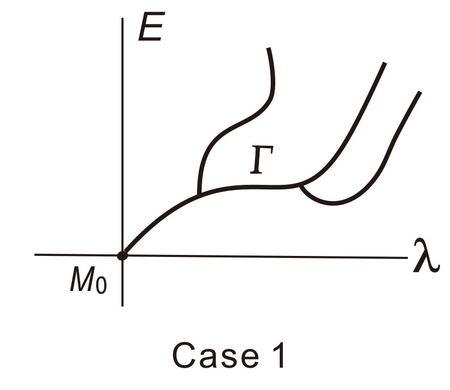 Figure 5
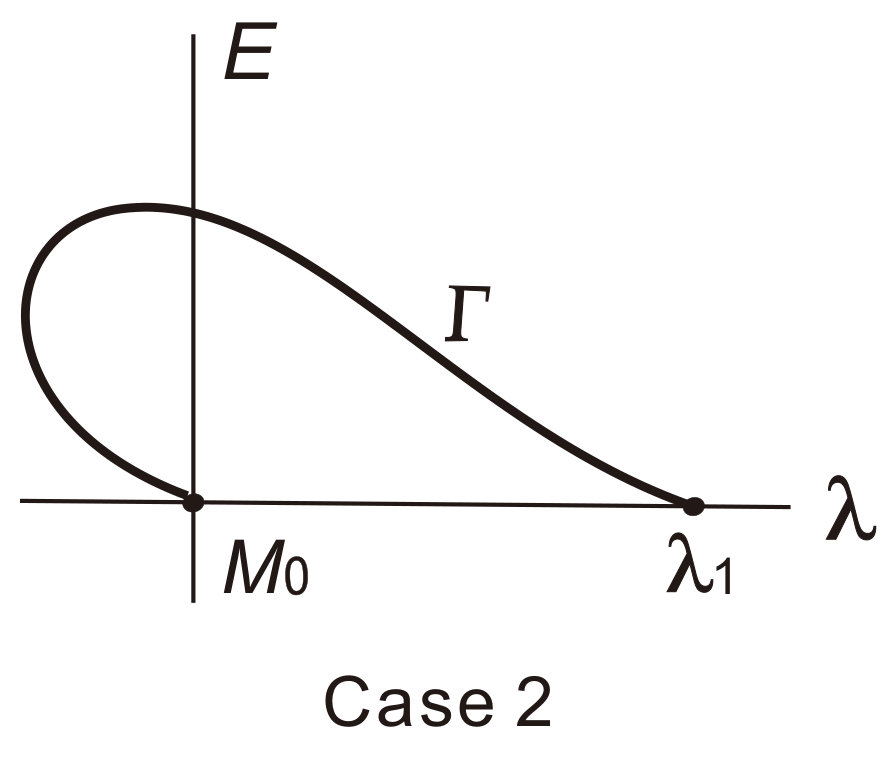 Figure 5
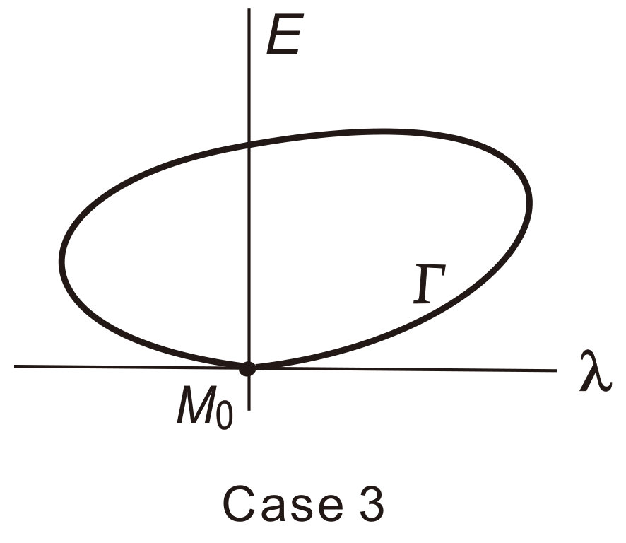 Figure 5
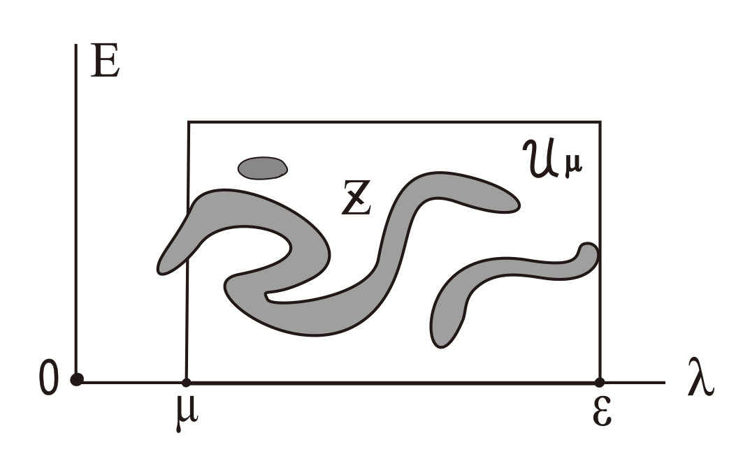 Figure 6
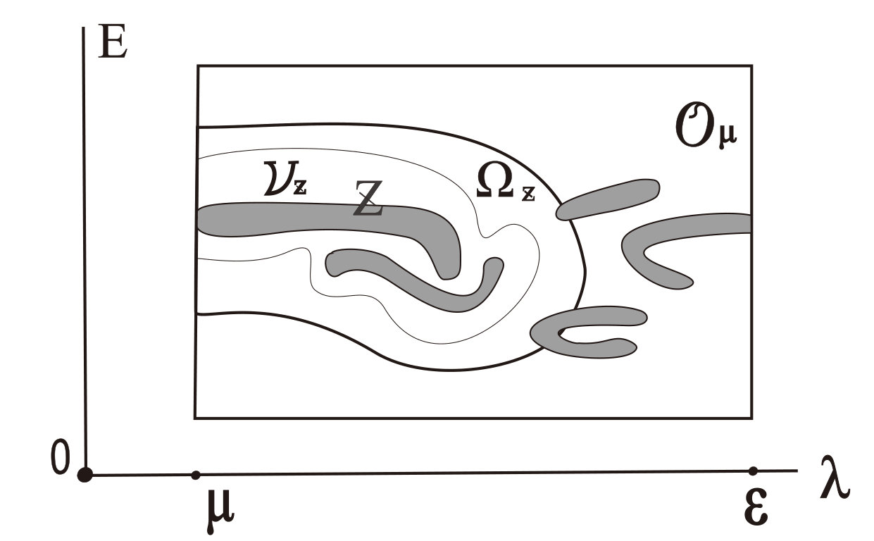 Figure 6
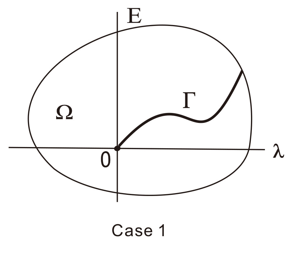 Figure 6
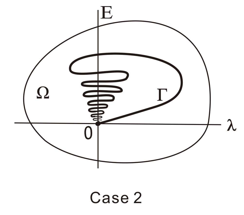 Figure 6
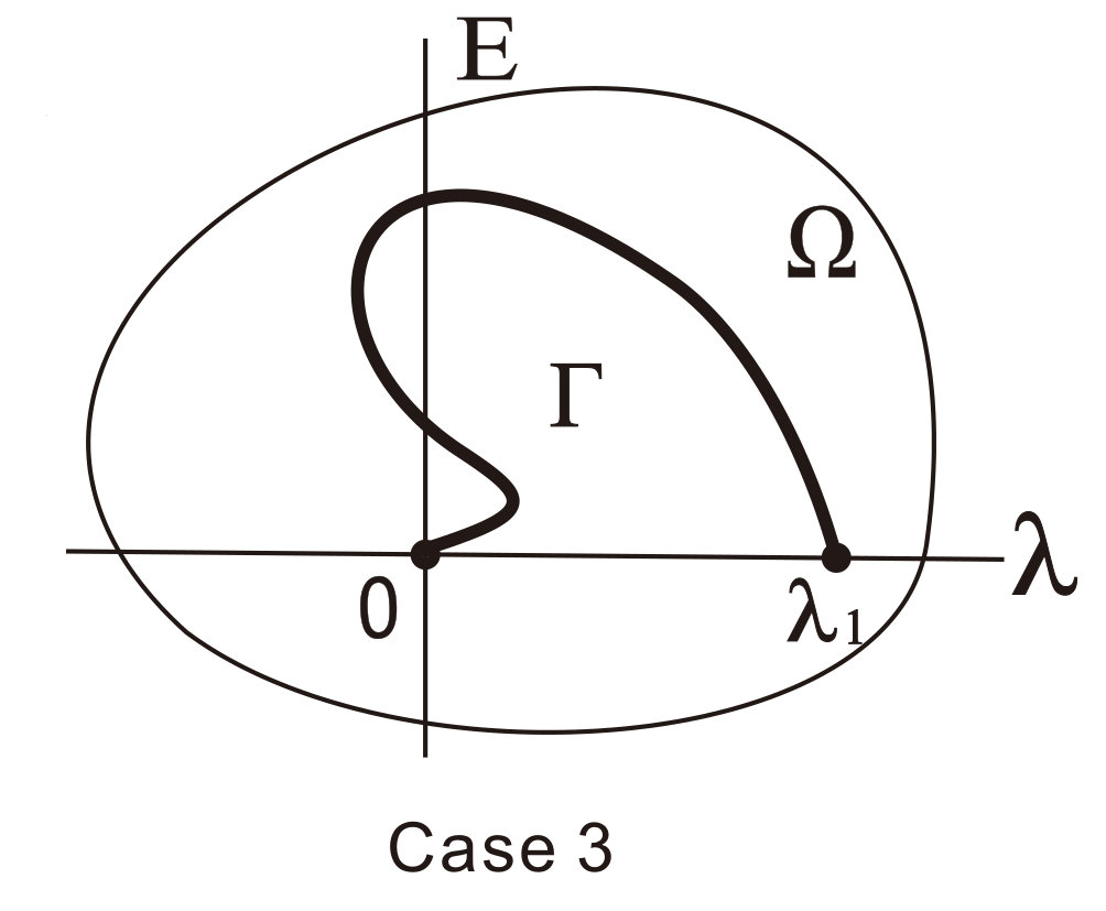 Figure 6
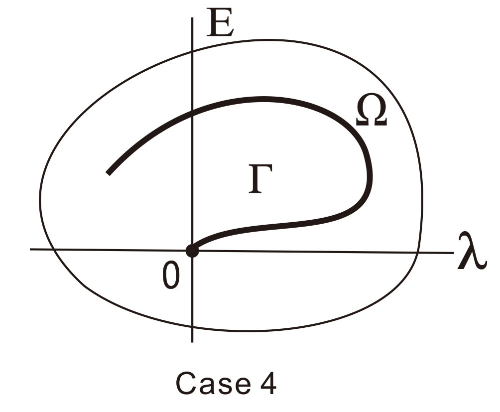 Figure 6
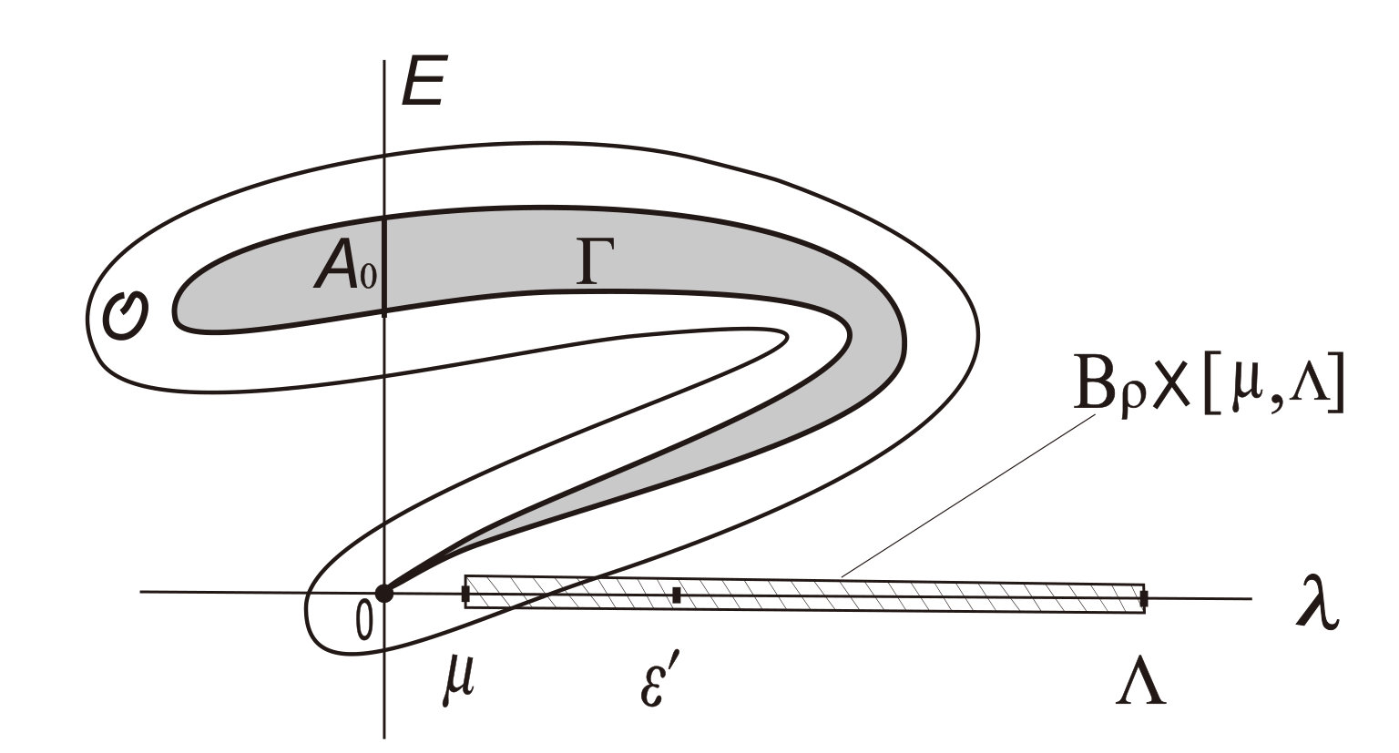 Figure 6
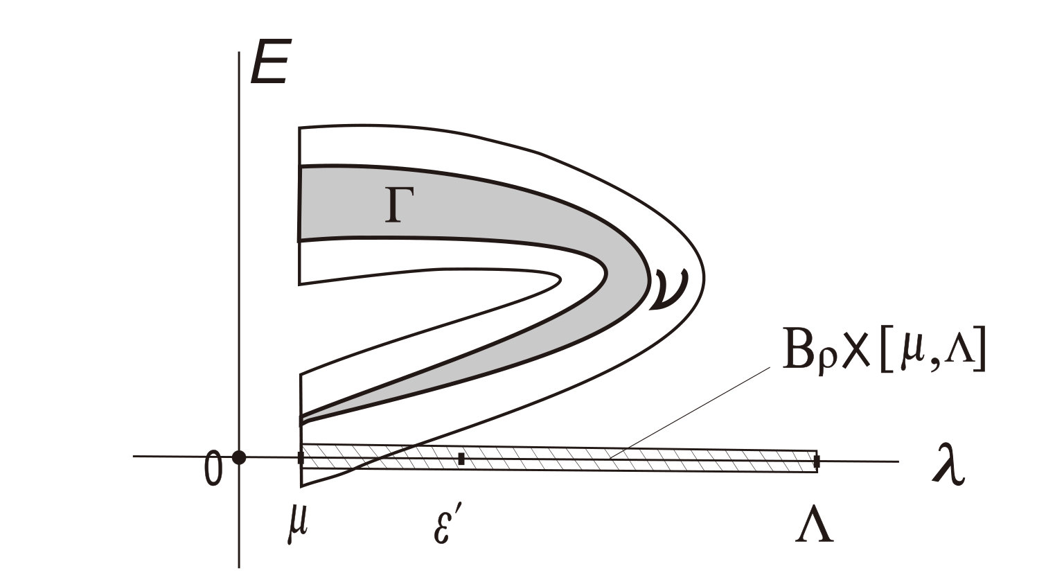 Figure 6
Peer Reviews
No public reviews on file for this paper yet. If you reviewed it on a platform where reviews are public (OpenReview, ICLR, NeurIPS, ICML), you can paste yours below so the community can read it here.
Videos
No videos yet. Explain this paper in a talk, walkthrough, or lecture? Add one.
Taxonomy
TopicsStability and Controllability of Differential Equations · Nonlinear Differential Equations Analysis · Mathematical and Theoretical Epidemiology and Ecology Models
**Equilibrium Index of Invariant Sets and Global
Static Bifurcation for Nonlinear
Evolution Equations**
Desheng Li 111Supported by the grant of NSFC (10771159, 11071185)
Department of Mathematics, Tianjin University
Tianjin 300072, China
E-mail: [email protected]
Zhi-Qiang Wang222Corresponding author, supported by the grant of NSFC (11271201)
Department of Mathematics and Statistics
Utah State University Logan, UT 84322
E-mail: [email protected]
Abstract. We introduce the notion of equilibrium index for statically isolated invariant sets of the system on Banach space (where is a sectorial operator with compact resolvent) and present a reduction theorem and an index formula for bifurcating invariant sets near equilibrium points. Then we prove a new global static bifurcation theorem where the crossing number may be even. In particular, in case , we show that the system undergoes either an attractor/repeller bifurcation, or a global static bifurcation. An illustrating example is also given by considering the bifurcations of the periodic boundary value problem of second-order differential equations.
1 Introduction
In our previous work [17] we studied the dynamic bifurcation of the equation
[TABLE]
on a Banach space , where is the bifurcation parameter, is a sectorial operator on with compact resolvent, and is a continuous mapping from to for some . Suppose for and hence is always a trivial equilibrium solution of (1.1). It was shown that if the crossing number at is nonzero (the “odd-multiplicity condition” is not needed), then the system bifurcates from the equilibrium solution [math] an isolated compact invariant set with nontrivial Conley index. Moreover, such a bifurcation enjoys some global features as in the classical Rabinowitz’s global static bifurcation theorem.
Now a natural problem arises: Does the bifurcated invariant set contain equilibrium solutions ? For gradient-like systems, this question seems to be somewhat trivial, as any nonempty compact invariant set of such a system necessarily contains an equilibrium. Another particular but important case is the one of the attractor bifurcation, for which Ma and Wang established some index formulas via indices of isolated singular points (see e.g. [22]). When the crossing number is odd, by using Ma and Wang’s index formulas one can assure the existence of equilibrium solutions in . Here we are interested in the general case. Our strategy is as follows.
First, we introduce the notion of equilibrium index for statically isolated invariant sets for the non-parameterized equation
[TABLE]
on , where is the same as in (1.1), and is a locally Lipschitz continuous mapping from to (). Denote the local semiflow generated by (1.2), and let be a statically isolated invariant set. We define the equilibrium index of an isolated invariant set to be the Leray-Schauder degree , where
[TABLE]
which maps into itself, is a real number such that , and is a statically isolating neighborhood of in . It can be shown that the index is independent of the choice of the number and the neighborhood , and hence is well defined. One of the advantages of introducing this notion is that, it allows us to obtain information on equilibrium solutions by directly performing some mathematical analysis on the evolution equation (1.2) without returning back to the corresponding stationary equation and putting it into a proper form so that one can apply the Leray-Schauder degree.
Secondly, we prove a reduction theorem for equilibrium index defined above by using the geometric theory of evolution equations, which allows us to compute the index of an invariant set near an equilibrium point by restring the system on the local center manifold of . More specifically, let be an equilibrium of . We show that there is a neighborhood of such that for any statically isolated invariant set of in , it holds that
[TABLE]
where is the dimension of the local unstable manifold of , and is the restriction of on the local center manifold. Since invariant manifolds are actually of a pure dynamical nature, the above result indicates that there are inherent connections between static and dynamic objects, which fact was recognized as early as in the work of Chow and Hale [6].
Thirdly, based on the reduction theorem and a result on the relation between topological degree and Conley index for finite dimensional systems given in Rybakowski [34], we establish an index formula for the bifurcating invariant set of (1.1). Denote the local semiflow generated by (1.1), and let be the restriction of on the local center manifold of [math]. Suppose is a dynamic bifurcation value, and let be the isolated invariant set bifurcated from the trivial equilibrium [math]. We prove that
[TABLE]
where and denote, respectively, the dimensions of the local unstable manifold and the local center manifold of [math] at ( is precisely the crossing number), and denotes the Euler number of the Conley index . Due to the degeneracy of the equilibrium [math] at , the computation of the index via topological degree seems to be of little hope. However, in some cases computing the Conley indices and may be of practical sense. For instance, in the particular case of attractor bifurcation, [math] is an attractor of the . Hence one easily deduces that
[TABLE]
where denotes the homotopy type of the pointed [math]-dimensional sphere (the space consisting of precisely two distinct points with one being the base point). Consequently . Thus for , by (1.3) we see that
[TABLE]
which, in our situation, recovers an index formula in the theory of attractor bifurcation given be Ma and Wang; see e.g. [21, Theorem 6.1]. Another important example is the one where and the equilibrium [math] fails to be an attractor of ; see Section 8 for details.
Fourthly, we are interested in the global static bifurcation of (1.1). A well-known result in this line is the famous Rabinowitz’s Global Bifurcation Theorem. However, it requires the crossing number to be odd (“crossing odd-multiplicity” condition). If one drops this condition then situations become very complicated. To the authors’ knowledge, even if for gradient systems the global static bifurcation still remains an open problem. To deal with this problem without assuming the “crossing odd-multiplicity” condition, Ma and Wang [20] proved some new local and global static bifurcation theorems by using higher-order nondegenerate singularities of nonlinearities. In this present work, motivated by the index formula (1.3) we give a new global static bifurcation theorem. Roughly speaking, we show that if is a bifurcation value and
[TABLE]
then the equation (1.1) bifurcates from the trivial stationary solution a connected branch of stationary solutions. (We call a stationary solution of (1.1) if is an equilibrium point of .) enjoys some global features as in the classical Rabinowitz’s Global Bifurcation Theorem. It is worth noticing that if the crossing number is odd, then the condition (1.5) is automatically satisfied.
Finally, we pay some special attention to the case where , i.e., there are exactly two eigenvalues (with multiplicity) crossing the imaginary axis. Let be a bifurcation point. Suppose is dynamically isolated with respect to the flow . We prove that the system either undergoes an attractor/repeller bifurcation (a generalized Hopf bifurcation), or bifurcates from a connected global bifurcation branch of stationary solutions. As an illustrating example, we consider the bifurcation of the periodic boundary value problem of the second-order differential equation
[TABLE]
where at . Let be the differential operator associated with periodic boundary condition. Then
[TABLE]
The first eigenvalue is simple with a corresponding constant eigenfunction, and all the others are of multiplicity . For each (), we show under appropriate conditions that either there is a two-sided neighborhood of such that for each , the problem has at least two distinct nontrivial solutions, or it bifurcates from a global bifurcation branch enjoying the properties in the Rabinowitz’s Global Bifurcation Theorem.
This paper is organised as follows. In Section 2 we make some preliminaries, and in Section 3 we introduce the notion of equilibrium index and discuss its basic properties. In Section 4 we establish a reduction theorem for equilibrium index. In Section 5 we give an index formula for the bifurcating invariant sets of (1.1). Section 6 is devoted to the global static bifurcation of (1.1), in which we prove a global static bifurcation theorem without the “odd-multiplicity condition”. Section 7 consists of some discussions on the special case where the crossing number . In Section 8 we give an illustrating example by considering the periodic boundary value problem of (1.6).
2 Preliminaries
This section is concerned with some preliminaries.
2.1 Basic topological notions and facts
Let be a metric space with metric . For convenience we will always identify a singleton with the point for any .
Let be a nonempty subset of . The closure, interior and boundary of are denoted, respectively, by , int and . A subset of is called a neighborhood of if . The -neighborhood of in , noted by , is defined to be the set
Let and be two nonempty subsets of . If then we will use the notations int and to denote the interior and boundary of in , respectively. The verification of the following basic facts is straightforward.
Lemma 2.1
. If then we also have .
The distance between and is defined as
[TABLE]
The Hausdorff semi-distance and distance of and are defined as
[TABLE]
respectively. We also assign .
Let () be a family of nonempty subsets of , where is a metric space. We say that is upper semicontinuous in at , this means
[TABLE]
The following two lemmas will play important roles in our discussion.
Lemma 2.2
[28]** Let be a compact metric space, and let , be two disjoint closed subsets of . Then either there is a subcontinuum of such that
[TABLE]
or , where and are disjoint compact subsets of containing and , respectively.
Lemma 2.3
[5]** (pp. 41) Let be a compact metric space. Denote by the family of compact subsets of which is equipped with the Hausdorff metric . Then is a compact metric space.
2.2 Some fundamental dynamical notions
In this subsection we collect some fundamental dynamical notions for the reader’s convenience.
Let be a metric space.
Definition 2.4
A local semiflow on is a continuous mapping from an open set to that enjoys the following properties:
- (1)
for each , there exists such that
[TABLE] 2. (2)
, and for all and with .
Assume that there has been given a local semiflow on . As usual we will write .
Let be an interval. A trajectory (or solution) of on is a continuous mapping such that
[TABLE]
A trajectory on is called a full trajectory.
A set is said to be positively invariant (resp. invariant), if (resp. ) for all .
A compact invariant set is said to be an attractor of , if it attracts a neighborhood of itself, namely,
The attraction basin of an attractor , denoted by , is defined as
[TABLE]
As in [13, Proposition 3.4], one can easily verify that is open.
Let be a compact invariant set. Then the restriction is a semiflow on . A compact set is said to be an attractor of in , this means that is an attractor of in .
Given an attractor of in , define
[TABLE]
is called the *repeller *of in dual to , and is called an attractor-repeller pair in .
A subset of is said to be admissible [34], if for any sequences and with , the sequence has a convergent subsequence. is said to be strongly admissible [34] if in addition, does not explode in , namely,
[TABLE]
Definition 2.5
* is said to be asymptotically compact on , if each bounded set is strongly admissible.*
Remark 2.6
If is asymptotically compact, then one easily verifies that each bounded invariant set of is necessarily precompact.
2.3 Conley index
From now on we assume that is a complete metric space. Although we don’t require to be complete in the definition of a local semiflow, completeness of the phase space always plays a crucial role in establishing a dynamical systems theory.
Let be a local semiflow on . Since we are working in an infinite dimensional space, in the remaining part of this section, we also assume that
- (AC)
is asymptotically compact.
A compact invariant set (we allow ) of is said to be isolated, if there exists a neighborhood of such that is the maximal invariant set in . Correspondingly, is called an isolating neighborhood of .
Let there be given an isolated invariant set . A pair of bounded closed subsets is called an index pair of , if (1) is an isolating neighborhood of ; (2) is -invariant, i.e., for any and ,
[TABLE]
(3) is an exit set of . Namely, for any , if for some , then there exists such that
Let be a closed domain. A point is called a strict egress (resp. strict ingress, bounce-off) point of , if for every trajectory with (where , and ),
- (1)
there exists such that
[TABLE] 2. (2)
if then there exists such that
[TABLE]
Denote (resp. , ) the set of all strict egress (resp. strict ingress, bounce-off) points of the closed set , and set
[TABLE]
A bounded closed domain is called an isolating block [34], if is closed and For an isolating block , we infer from [34] that is an index pair of the maximal compact invariant set (possibly empty) in .
Definition 2.7
(homotopy index) Let be an index pair of . The homotopy Conley index of is defined to be the homotopy type of the pointed space , denoted by .
Remark 2.8
Denote and the singular homology and cohomology theories with coefficient group , respectively. Applying and to one immediately obtains the homology and cohomology Conley index and , respectively.
An important property of the Conley index is the homotopy invariance of the index. Here we state a result in this line for the reader’s convenience, which is actually a particular case of [34, Chap. I, Theorem 12.2].
Let () be a family of asymptotically compact local semiflows on , where is a metric space. We say that depends on continuously, if is defined at , then for any sequence converging to , is also defined for all sufficiently large, furthermore,
[TABLE]
Suppose the family () depends on continuously. Set
[TABLE]
Then is a local semiflow on the product space . For convenience, we call the skew-product flow of the family.
We say that is -locally uniformly asymptotically compact (-l.u.a.c. in short), if the skew-product flow is asymptotically compact. It is easy to see that if is -l.u.a.c., then the parameter space is necessarily locally compact.
Suppose for each , has an isolated invariant set . We call the pair a dynamic continuation on , if for every , there is a neighborhood of in and a set such that is an isolating neighborhood of for all . In the case where is -l.u.a.c., one can easily verify that a dynamic continuation is -continuous in the terminology of [34, Chap. I, Def. 12.1]. Hence by [34, Chap. I, Theorem 12.2] we have
Theorem 2.9
Assume that is -l.u.a.c. Let be a dynamic continuation on . Then is constant for in any component of .
3 Equilibrium Index of Statically Isolated Sets
Let be a Banach space with norm , and be a sectorial operator on with compact resolvent. Denote () the fractional powers of induced by equipped with the usual norm (see [10, Chap. 1] for details). Consider the equation
[TABLE]
where is an open subset of for some fixed . Our main purpose in this section is to introduce the notion of equilibrium index for (3.1).
For convenience in statement, we will write , meaning that is a bounded subset of with
[TABLE]
We always assume is locally Lipschitz continuous, namely,
- (LC)
for any , there exists such that
[TABLE]
Under the above assumption, it is well known that the initial value problem of the equation is well-posed. That is, for each the problem has a unique solution with defined on a maximal existence interval with ; see e.g. [10, Chap. 3]. Define a local semiflow on as
[TABLE]
is usually called the local semiflow generated by (3.1).
Remark 3.1
Note that in general the domain may not be complete. However, one easily understands that the dynamical systems theory reviewed in Section 2 applies to quite well on any closed domain .
3.1 Definition of the equilibrium index
Given , denote the set of equilibrium points of in .
Definition 3.2
A set is called statically isolated if it has a neighborhood such that Correspondingly is called a statically isolating neighborhood of .
For convenience in statement, given and , we write
[TABLE]
meaning that for all
Take a number with . Let
[TABLE]
Then is pre-compact in for any .
Definition 3.3
Let be statically isolated with being an isolating neighborhood. The equilibrium index of , denoted by , is defined as
[TABLE]
where denotes the Leray-Schauder degree.
It is trivial to verify that the definition of is independent of the choice of and the number .
A basic property of the equilibrium index is that it is invariant under transformations. Specifically, let be another Banach space. Suppose there is an isomorphism (a bounded linear bijection with bounded inverse). Consider the following equation:
[TABLE]
where , and Denote the local semiflow generated by (3.2). Then and are conjugate, namely, . We have
Proposition 3.4
Let be a statically isolated set of . Then is a statically isolated set of ; furthermore,
[TABLE]
Proof. Take a number so that . Let Then (3.2) can be written as
[TABLE]
where
[TABLE]
We have
[TABLE]
Pick an (statically) isolating neighborhood of . Then is an isolating neighborhood of . Hence by definition we have
[TABLE]
which completes the proof of the result.
3.2 Continuation property
Let , and be as above. Consider the equation with parameter :
[TABLE]
where is a connected compact metric space. Instead of (LC) we assume that
- (UL)
for any and compact subset of , there exists such that
[TABLE]
Denote the local semiflow generated by (3.6) on . It is easy to verify that depends on continuously.
Let be skew-product flow of the family () on . Clearly is an equilibrium of iff is an equilibrium of .
The following result is a simple consequence of the continuation property of the Leray-Schauder degree.
Theorem 3.5
Let be a statically isolated set of the skew-product flow in . Set . Then remains constant for .
Proof. Since is a statically isolated set of , by definition has a bounded closed isolating neighborhood . Note that , where denotes the boundary of in . It is trivial to check that . Therefore we deduce that
[TABLE]
Hence we can pick a bounded closed set such that for all .
Using local Lipschitz continuity of one easily verifies that \begin{array}[]{ll}\bigcup_{\lambda\in\Lambda}f_{\lambda}\left(B\right)\end{array} is bounded in . Consequently is a bounded set in . Let
[TABLE]
Then the set \begin{array}[]{ll}\bigcup_{\lambda\in\Lambda}F_{\lambda}(B)=(aI+A)^{-1}M\end{array} is bounded in . As has compact resolvent, the embedding is compact. Therefore is precompact in . Now by virtue of continuation property of the Leray-Schauder degree we immediately concludes that
[TABLE]
on . The proof of the theorem is complete.
Suppose has a statically isolated invariant set for each (we allow ). We say that is a static continuation on , if for each , there exist and a neighborhood of in such that is a statically isolating neighborhood of for all .
Theorem 3.6
Let be a static continuation on . Then remains constant on . In particular, if then
Proof. To prove Theorem 3.6, it suffices to check that for any , there is a neighborhood of in such that
[TABLE]
Let . Then by the definition of a static continuation, one can find a neighborhood of and a neighborhood of in such that is a statically isolating neighborhood of for all . Pick a connected compact neighborhood of with . One easily sees that is a static isolated set of the skew-product flow of (). Applying Theorem 3.5 we immediately conclude the validity of (3.5).
3.3 The finite dimensional case
Now we assume is an -dimensional Banach space. Consider the ODE system:
[TABLE]
where is locally Lipschitz. Denote the semiflow generated by (3.6).
Proposition 3.7
Let be a statically isolated set of . Then
[TABLE]
for any isolating neighborhood of .
If is an isolated invariant set of , we also have
[TABLE]
where is the Euler number of the Conley index .
Proof. We may assume . Take an arbitrary -matrix and rewrite (3.6) as
[TABLE]
where . Pick a number so that . Then
[TABLE]
Note that implies . Further by the definition of the Brouwer degree it is easy to deduce that
[TABLE]
Hence
[TABLE]
Now assume that is an isolated invariant set of . Pick an (dynamically) isolating neighborhood of . Then we infer from Reineck [33] (see also [32, Theorem 3.2]) that can be continued in to an isolated invariant set of a flow generated by
[TABLE]
where is a Morse-Smale gradient vector field on a neighborhood of with , and on . Thus by Rybakowski [34, Chap. III,Theorem 3.8] (see also Chang [3, Chap. II, Theorems 3.1-3.3]) one concludes that
[TABLE]
The proof is complete.
Remark 3.8
In [32] the Euler number is defined to be the Poincaré index of (see [32, Section 3]).
4 Invariant Manifolds of Nonlinear Equations
For completeness and the reader’s convenience, in this section we briefly recall some results on local invariant manifolds of the following nonlinear evolution equation with parameter :
[TABLE]
where is a sectorial operator in with compact resolvent, and is a continuous mapping from to for some .
Without loss of generality, assume that for hence is always an equilibrium solution of (4.1).
Assume that is locally Lipschitz in ; furthermore, the local Lipschitz continuity assumption (UL) in Subsection 3.2 is fulfilled. Denote the local semiflow generated by (4.1). Then we know that depends on continuously. Also, by very standard argument (see e.g. [34, Chap. I, Theorem 4.4]), it can be shown that is -l.u.a.c. on .
4.1 Fundamental assumptions and notations
Let , and write
[TABLE]
Then (4.1) reads
[TABLE]
Suppose there exists such that the following hypotheses (H1)-(H3) are fulfilled for every :
- (H1)
The spectral has a decomposition such that
[TABLE]
for some (independent of ). 2. (H2)
The space has a decomposition corresponding to the decomposition of in (H1), such that are -invariant subspaces of . Moreover,
[TABLE] 3. (H3)
The projection operators
[TABLE]
are continuous in .
Remark 4.1
The above assumptions implies that there is a family () of isomorphisms on depending continuously on with , such that
[TABLE]
see Appendix A for the proof. It is trivial to verify that for all
Let
[TABLE]
and denote the projection from to . Then . We infer from Remark 4.1 that
[TABLE]
We will rewrite . Let
[TABLE]
Then
[TABLE]
Because and are finite dimensional, we actually have
[TABLE]
For notational simplicity, hereafter we write
[TABLE]
[TABLE]
Denote the ball in centered at [math] with radius , and set
[TABLE]
Lemma 4.2
For any neighborhood of [math] in , there exists such that
[TABLE]
Proof. Since is a neighborhood of [math] in , we can pick an sufficiently small so that for . Further by using compactness of () one can easily verify that there exists such that , from which (4.7) immediately follows.
4.2 Local invariant manifolds
Let us recall briefly some fundamental results on local invariant manifolds.
Let be the isomorphism on given in Remark 4.1. Setting , system (4.2) is transformed into an equivalent one:
[TABLE]
where
[TABLE]
It is easy to verify (or see [17, Section 3]) that
Denote the local semiflow generated by (4.8).
Since () are -invariant, by (4.5) we find that () are -invariant for all . Thus by (4.3) we deduce that
[TABLE]
where is the restriction of on . Now the same arguments as in the proofs of Lemmas 3.3 and 3.4 in [17] apply to prove the following theorem.
Theorem 4.3
There exist open convex neighborhoods of [math] (independent of ) in such that the following assertions hold.
There is a continuous mapping from to which is differentiable in with being continuous in and such that for each , the set is a local invariant manifold of system (4.8). 2.
There is a continuous mapping from to which is differentiable in with being continuous in and such that for each , the set is a local invariant manifold of (4.8), where
[TABLE] 3.
* is an isolated invariant set of the semiflow of (4.8) iff * ( resp. ) and is an isolated invariant set of ( resp. ). Furthermore,
[TABLE]
Remark 4.4
Assertions (1) and (2) are only slight modifications of some classical results in the geometric theory of evolution equations (see e.g. [34, Chap. II, Theorem 2.1]). A sketch of the proof can be found in [17]. (3) is a parameterized version of a corresponding result in [34, Chap. II, Theorem 3.1].
Remark 4.5
Using and it is easy to deduce that for any , there exists such that
[TABLE]
for all B, and . It follows that
[TABLE]
uniformly with respect to .
Remark 4.6
It is known (see e.g. [34, Section 2.2]) that satisfies equation
[TABLE]
for , and satisfies
[TABLE]
for . Here (and below) and
[TABLE]
Let
[TABLE]
Define and as below:
[TABLE]
[TABLE]
As a direct consequence of Theorem 4.3, we have the following.
Theorem 4.7
Assume the hypotheses (H1)-(H3). Then
the following two sets are local invariant manifolds of system (4.1):
[TABLE]
[TABLE] 2.
* ( where ) is an isolated invariant set of the semiflow of (4.1) iff * ( resp. ) and is an isolated invariant set of ( resp. ). Furthermore,
[TABLE]
Let be a solution of (4.2) (or (4.1)) lying in , where
[TABLE]
Then , and therefore satisfies
[TABLE]
Similarly one can also obtain the equation corresponding to :
[TABLE]
(4.19) and (4.20) will be referred to as the reduction equations of (4.2) (or (4.1)) on and , respectively.
Denote and the local semiflow on and generated by (4.19) and (4.20), respectively. Then and conjugate with and , respectively. More precisely, we have
[TABLE]
[TABLE]
Remark 4.8
By (4.22), (4.22) and Theorem 4.7 it is easy to see that is an (isolated) invariant set of iff (resp. ) is an (isolated) invariant set of (resp. ).
5 Reduction Theorem of Equilibrium Index near Equilibrium Points
Our main purpose in this section is to establish a reduction theorem for equilibrium indices of isolated invariant sets of system (4.1) near equilibrium points.
We follow the same notations as in Section 4 and assume the function in (4.1) satisfies all the regularity hypotheses in Section 4. Suppose also that for . The main result is the following theorem.
Theorem 5.1
Assume the hypotheses (H1)-(H3) in Section 4 are fulfilled. Then there exists an open neighborhood of [math] in (independent of ) such that for every isolated invariant set of in , we have
[TABLE]
where .
Proof. Some basic ideas and techniques used here are borrowed from [34] (see [34, Chap. II, Theorem 3.1] and its proof).
For notational simplicity, in the following we will drop the subscript “” and simply rewrite , , , , and as , , , respectively, unless we need to emphasize the dependence on . We split the argument into several steps. *Step *1. We begin with system (4.8). Let () be the neighborhood of [math] in given in Theorem 4.3, and let
[TABLE]
For each fixed , define a family of mappings () as
[TABLE]
Note that if then
[TABLE]
Using the same argument as in Step 1 in the proof of [34, Chap. II, Theorem 3.1], one can easily verify that is open; furthermore, has a continuous inverse given by
[TABLE]
where , and . (Here and below and denote and , respectively, except otherwise statement.)
Note that depends upon and continuously. Consequently is continuous in (, ) in the sense of Hausdorff distance. Using this simple fact one easily checks that there is a neighborhood of [math] in such that
[TABLE]
By Lemma 4.2 we can pick a number such that
[TABLE]
( denotes the ball in ). In view of (4.13), it can be assumed that is chosen sufficiently small so that for all , we have
[TABLE]
Define a local semiflow on to be the “ image” of the local semiflow of (4.8) under , namely,
[TABLE]
Then by (5.4) is well defined on the domain for all and . Making us of the relation in (4.14), it can be shown by some simple computations that is precisely the local semiflow generated by system
[TABLE]
where , , , and
[TABLE]
Note that (5.5) reduces to system (4.8) when . Hence coincides with .
Take a number (independent of and ) such that and
[TABLE]
Let be an isolated invariant set of , and write
[TABLE]
Then (5.6) implies that is an isolated invariant set of in for all (and ). It is trivial to verify that is a static coninuation. Thus by Theorem 3.6 we deduce that
[TABLE]
Step 2. For , system (5.5) reads
[TABLE]
where
[TABLE]
Since , it is clear that
[TABLE]
Consider on the domain the homotopy of system (5.8):
[TABLE]
Lemma 5.2
There exist a small open neighborhood of [math] in with and constants such that for all and , if is a solution of (5.10) on lying in then
[TABLE]
Proof. The proof is a slight modification of that of [34, Chap. II, Lemma 3.3]. We omit the details. Denote the local semiflow on generated by (5.10). Then (5.9) implies that is a local invariant manifold of for all . Further by (5.9) and (5.10) we deduce that is actually independent of .
On the other hand, if is an invariant set of , then by Lemma 5.2 we find that . Using this fact and the independence of upon it is easy to see that all the local semiflows () share the same invariant sets in . Consequently is an isolated invariant set of for some iff it is an isolated invariant set of for all .
Now we pick a positive number such that
[TABLE]
Let be an isolated invariant set of . Then
[TABLE]
is an isolated invariant set of in . (The second equality in (5.12) follows from (5.3) and the fact that .) Since coincides with , by what we have proved above we see that is an isolated invariant set of for all . Further one can easily verify that is a static coninuation. Thus by Theorem 3.6 and (5.7) we obtain that
[TABLE]
where is the local semiflow on generated by the system
[TABLE]
Step 3. We now calculate the index . For this purpose, consider the following homotopy of system (5.14):
[TABLE]
where . Since (see (4.10)), we have
[TABLE]
Denote the local semiflow generated by (5.15). Then . Hence is an isolated invariant set for . Further repeating the same argument as above with minor modifications it is easy to deduce that is an isolated invariant set of for all . Now as in the preceding steps, by Theorem 3.6 we get
[TABLE]
Step 4. For , (5.15) reads
[TABLE]
An equivalent form of the system reads
[TABLE]
where . Take a number sufficiently large so that has bounded inverse . Rewrite (5.18) as
[TABLE]
Since commutes with , by (4.6) it is trivial to verify that commutes with for all . Hence . Using this fact one can easily show that is invertible with
[TABLE]
Define an operator on as
[TABLE]
Then
[TABLE]
Hence is a finite dimensional operator. Therefore by the definition of the equilibrium index and the reduction property of the Leray-Schauder degree, we deduce that
[TABLE]
where is a closed isolating neighborhood of , and . Thus by (5.13) and (5.16) we have
[TABLE]
Denote the local semiflow generated by the first equation in (5.17):
[TABLE]
( is well-defined on .) As in Remark 4.8 we know that is an isolated invariant set of with being an isolating neighborhood. Hence we have
[TABLE]
where
[TABLE]
On the other hand, it is trivial to verify that Therefore
[TABLE]
Combing this with (5.22) and (5.20) one concludes that
[TABLE]
Step 5. Now we pay some attention to the calculation of . At this point, we are in a quite similar situation as we were at the beginning of calculating the index with system (4.8) replaced by (5.21).
Write , where . Then (5.21) can be reformulated as
[TABLE]
Repeating a similar argument as in Steps 1 and 2 leading to (5.13) with some corresponding modifications, it can be shown that there exists (independent of ) such that for any isolated invariant set of (5.21) with ,
[TABLE]
where is the local semiflow generated by
[TABLE]
where is the *invariant manifold * mapping given in (4.11).
Let
[TABLE]
Pick a closed isolating neighborhood of with . Recalling that , a simple calculation yields
[TABLE]
where is the local semiflow on generated by the system
[TABLE]
Step 6. We first take a positive number such that , where is the neighborhood of [math] given in Lemma 5.2. Then choose a positive number ( is the number in (5.11)) small enough so that
[TABLE]
where is the mapping defined in (5.2).
Let be an isolated invariant set of in . Clearly
[TABLE]
Since (see (5.12)), the inclusion implies that
[TABLE]
Thus by (5.23) and (5.27) we obtain that
[TABLE]
Step 7. Let . By continuity of in one can easily verify that there exists a neighborhood of [math] in such that for all . Take a number sufficiently small such that ; furthermore,
[TABLE]
The reduction equation (4.20) on reads
[TABLE]
where , , and . Write
[TABLE]
Noticing that (recall that ), we find that
[TABLE]
where , and is the function in equation (4.8). Since , by Proposition 3.4 we deduce that for any isolated invariant set of the local semiflow of (5.28), one has
[TABLE]
where is the local semiflow of (4.20) on .
Now let be an isolated invariant set of . Set . Then by Proposition 3.4 and (5.30) we conclude that
[TABLE]
which completes the proof of the validity of the second equality in (5.1). (The last equality in (5.32) is due to the fact that .)
The first equality in (5.1) follows from Proposition 3.4 and the first equality in (5.30). The proof of the theorem is complete.
6 An Index Formula for Bifurcating Invariant Sets near Equilibrium Points
As in Section 5, we follow the same notations as in Section 4 and assume the function in (4.1) satisfies all the regularity hypotheses in Section 4. Suppose also that for . The main result is the following theorem.
Theorem 6.1
In addition to (H1)-(H3) (see Section 4), assume that
- (H4)
for , we have
[TABLE]
Suppose also that is an isolated invariant set of .
Then there exist closed isolating neighborhood of with respect to and such that has a maximal compact invariant set ( may be void) in for each , . Furthermore,
[TABLE]
where , and .
Remark 6.2
The interested reader is referred to [17, Theorem 4.3] on when the bifurcating invariant set is nonvoid. We also infer from the proof of [17, Theorem 4.3] that is upper semicontinuous in .
Remark 6.3
For convenience, we will call the number in Theorem 6.1 the crossing number at in case (H4) is fulfilled.
Proof of Theorem 6.1. (1) Pick a closed isolating neighborhood of with , where is the neighborhood of [math] given in Theorem 5.1. Then by a very standard argument (see e.g. [34, Chap. I]) it can be shown that there exists such that is an isolating neighborhood of for all . Denote the maximal compact invariant set of in . Then we infer from Theorem 4.7 that and is an isolated invariant set of on .
For convenience in statement, let us temporarily forget the conjugacy between and the local semiflow of the reduction equation (4.20) and identify the two local semiflows.
Let . Then by (H4) we deduce that , where is the linear operator in the reduction equation (4.20). Hence is a repeller of . It follows by the standard Morse decomposition theory of invariant sets that has a Morse decomposition with . Note that is the maximal compact invariant set of in . By maximality of it can be easily seen that is also the maximal compact invariant set of in . (It may occur that . In such a case we have .)
If then is an attractor of , and a parallel argument applies to show that has a maximal compact invariant set in .
(2) Let be the maximal compact invariant set of in . Since , we can pick a with such that , where denotes the ball in centered at [math] with radius . Then is a closed neighborhood of . Further by maximality of in we deduce that is an isolating neighborhood of .
We infer from the Morse decomposition theory that is the union of , and the connecting orbits between and . Thus one concludes that (Recall that denotes the set of equilibrium points in .) Therefore
[TABLE]
On the other hand, by homotopy property of the equilibrium index we have
[TABLE]
Hence by (5.1) and Proposition 3.4 we deduce that
[TABLE]
It then follows by (6.2) that
[TABLE]
Simple calculations show that
[TABLE]
Therefore
[TABLE]
We also infer from (6.3) that
[TABLE]
Combining this with (6.2) and (6.5) one immediately concludes the validity of the second equality in (6.1).
7 A Global Static Bifurcation Theorem
We follow the same notations in the preceding sections. Furthermore, we assume the function in (4.1) satisfies all the regularity hypotheses in Section 4.
Let . is equipped with metric defined as
[TABLE]
Given and , denote the -section of :
[TABLE]
Let be the local semiflow of (4.1), and denote the skew-product flow of the family () on ,
[TABLE]
As in the proof of Theorem 3.5 it can be shown that the set is bounded in for any bounded subset of . Using this simple fact and applying some fundamental theory on abstract evolution equations (see e.g. [10, Chap. 3] and [34, Chap. I, Theorem 4.4]), it can be shown by very standard argument that is asymptotically compact. Consequently each bounded closed invariant set of is necessarily compact.
Assume for all , hence is always a trivial equilibrium of . Given , denote
[TABLE]
Definition 7.1
Let be a closed neighborhood of . The (static) bifurcation branch of from in is defined to be the component of which contains .
7.1 Existence of local bifurcation branch
Let us first give an existence result of a nontrivial local bifurcation branch.
Let and be the local invariant manifolds of given in Theorem 4.7, and denote , .
Theorem 7.2
Assume (H1)-(H4) (see Section 4 and Theorem 6.1) are fulfilled. Suppose is an isolated invariant set of , where is the number appearing in (H4). Let be the isolating neighborhood of given in Theorem 6.1. Then there exists such that the following assertions hold.
If then . 2.
If then
Here , and .
Proof. For simplicity, we set . Choose an such that the assertions in Theorem 6.1 hold. Let be the maximal compact invariant set of in , and the maximal compact invariant set of in . We may restrict small enough so that is an isolating neighborhood of for all .
For definiteness we assume and prove that
[TABLE]
Let us first show that for any , there is a component of , where , such that
[TABLE]
Set , and let . Then is a bounded invariant set of the skew-product flow . By upper semicontinuity of in (see Remark 6.2) one can easily verify that is closed. Remark 2.6 then asserts that is compact in . As for , we have
[TABLE]
It is also trivial to deduce that . Pick a number . Then is a closed isolating neighborhood of for all .
Take a number sufficiently large so that . Set
[TABLE]
As in the proof of Theorem 3.5 we know that is precompact in for any bounded subset of .
We infer from Theorem 6.1 that
[TABLE]
This allows us to apply the classical Leray-Schauder continuation theorem (see e.g. Mawhin [23, Section 2]) to deduce that there is a component such that , from which (7.2) immediately follows.
We are now ready to complete the proof of the theorem. Take a sequence of positive numbers . For each , pick a connected component of such that \begin{array}[]{ll}{\mathcal{Z}}_{k}[\mu_{k}]\neq\emptyset\neq{\mathcal{Z}}_{k}[\varepsilon].\end{array} By Lemma 2.3 we may assume that converges in the sense of Hausdorff distance to a compact set . Then is a continuum in with . On the other hand, by the choice of we have . Therefore one concludes that .
7.2 Global static bifurcation theorem
For simplicity, in this subsection we rewrite . Given and , we also denote
[TABLE]
Let be a bifurcation point.
Definition 7.3
The global (static) bifurcation branch of is defined to be the bifurcation branch of in .
The right-hand side global bifurcation branch of is defined as
[TABLE]
where denotes the bifurcation branch of in .
Similarly one can define the left-hand side global bifurcation branch .
Remark 7.4
One easily verifies that both and are connected; moreover, we have .
Our main result in this section is the following global bifurcation theorem.
Theorem 7.5
Assume (H1)-(H4) are fulfilled. Suppose is an isolated invariant set of ; furthermore,
[TABLE]
Then one of the following cases occurs (see Figures 6.3-6.5).
* is unbounded. * 2.
There exists such that . 3.
, in which case both and return back to .
Figure 6.3: is unbounded. Figure 6.4: connects to .
Figure 6.5: return back to .
Proof. We may assume . We argue by contradiction and suppose that none of the cases (1)-(3) occurs. Then both are bounded closed subsets of . Moreover,
[TABLE]
[TABLE]
see Fig. LABEL:fig7-4. By asymptotic compactness of we know that are compact.
Step 1. By Theorem 7.2 we have either , or . Let
[TABLE]
We may assume In the case when or , the argument is simpler and can be obtained by slightly modifying the one below. In the following we first show that and are closed and hence are compact. For this purpose it suffices to check that is an isolated point in both the sets and .
We argue by contradiction and suppose that is not isolated in, say, . Then there exists a sequence converges to . Since is an isolated equilibrium of , it is clear that (hence ) for all sufficiently large.
Pick a closed statically isolating neighborhood of [math] with respect to . There is such that is statically isolating with respect to for . It can be assumed that and for all .
Denote the continuum of containing . If then by definition we find that . Hence , which contradicts (7.5). Thus we deduce that . As is the only equilibrium of in , it follows that Further, because , by connectedness of one concludes that .
By Lemma 2.3 we may assume that converges in the sense of Hausdorff distance to a compact subset . Then is a continuum in . Clearly and . Hence for all . We infer from (7.4) that
[TABLE]
Thereby . But this and (7.6) contradict (7.5).
Step 2. By (7.4) and the definition of and it is clear that for all . Thus by compactness of and , there exists such that
[TABLE]
Let and be given as in Theorem 6.1. We may assume is chosen sufficiently small so that . Clearly
[TABLE]
see Fig. LABEL:. Pick a number with . Denote the maximal invariant set of in . Since
[TABLE]
there exists such that
[TABLE]
By compactness of it is easy to verify that are upper semicontinuous in . Thus we can restrict sufficiently small so that
[TABLE]
[TABLE]
(Note that , and .) Let
[TABLE]
By (7.7), (7.11), (7.12) and the choice of we clearly have
[TABLE]
Thus by (7.5) one finds that and The choice of and (7.7) also imply
[TABLE]
where . Therefore we can pick a such that
[TABLE]
and
[TABLE]
It is easy to check that
[TABLE]
Let . Then since , it follows from (7.16) that
[TABLE]
Step 3. By (7.9) there is with such that
[TABLE]
where is the maximal invariant set of in .
Let . Then by compactness of we deduce that is a compact subset of . As , one has
[TABLE]
Take a number By some standard argument (see e.g. the proof of [17, Theorem 6.2], one can find a bounded closed neighborhood of with such that
[TABLE]
Let
[TABLE]
Define
[TABLE]
We infer from (7.14) and (7.15) that , and are disjointed. Recalling that and , one trivially verifies that
[TABLE]
Furthermore, the following basic facts hold true.
Lemma 7.6
Let and . Then
[TABLE]
[TABLE]
[TABLE]
where denotes the ball in of center [math] and radius .
Proof. (1) As , the inequality (7.25) directly follows from (7.13).
(2) Note that for all . Thus by (7.10) we have . Observing that if then
[TABLE]
one concludes that from which (7.23) immediately follows.
(3) It is obvious that . So we only need to verify the converse inclusion for each . For this purpose, it suffices to check that if and then .
Indeed, let , . Then for any with , we have
[TABLE]
Therefore since , we deduce that Thus by (7.17) one has
[TABLE]
which implies
[TABLE]
Hence by (7.21) we see that . This finishes the proof of (7.24).
Step 4. For the sake of definiteness, we assume
[TABLE]
and focus our attention on the interval . Because is a neighborhood of in , there exist such that i.e.,
[TABLE]
By (7.9) we can find a number such that
[TABLE]
where is the bifurcating invariant set given in Theorem 6.1.
Let . Then as in (7.3) we deduce that
[TABLE]
Take a number such that
[TABLE]
Let , where is the number given in (7.19). Let , and define
[TABLE]
Clearly is closed in . Since is open in , we see that is closed in as well. We claim that
[TABLE]
To see this, by definition it suffices to show that if , then any equilibrium of in is contained in .
Figure 6.7 Figure 6.8
We first consider . Because contains all nonzero equilibria of in , in this case one finds (by the choice of ) that there are no equilibrium points of in other than [math]. Thus by the definition of we see that .
Now assume . We show that , hence , and the conclusion immediately follows. Let . As , there is a such that
[TABLE]
which implies (otherwise ). Hence by (7.19) we have . Therefore
[TABLE]
We thus infer from the choice of that . This verifies that and completes the proof of (7.30).
It is trivial to check that is a neighborhood of in . Pick a number sufficiently small so that is a neighborhood of in . Theorem 3.5 then asserts that
[TABLE]
On the other hand, if then
[TABLE]
Setting
[TABLE]
one obtains that
[TABLE]
for . It follows by (7.31) that
[TABLE]
We infer from (7.28) and the choice of that for . Recalling that contains all nontrivial equilibria in (and hence in ) and noticing that , we deduce that
[TABLE]
Thus by (7.32) we have
[TABLE]
Step 5. Finally we show that the left-hand side of (7.33) equals [math], thus obtain a contradiction. For this purpose, consider the domain in defined in (7.21). Let , where , and is the number in (7.29). We claim that the boundary of in contains no equilibrium points. To see this, by (7.20) it suffices to check that .
Indeed, since , we infer from Lemma 2.1 that
[TABLE]
On the other hand, by (7.22) we find that where . Therefore by Lemma 2.1 we deduce that
[TABLE]
Hence .
Let . Then is a compact invariant set of the skew-product flow of the family () on . We infer from the claim proved above that . Hence is a static isolating set of . Thanks to Theorem 3.5,
[TABLE]
Therefore
[TABLE]
A parallel argument as above applies to show that for Finally combining the above results with (7.33) we conclude . This and (7.26) contradict Theorem 6.1.
The proof of the theorem is finished.
Remark 7.7
If the third case (3) in Theorem 7.5 occurs then both are nontrivial; furthermore, we have . Therefore as depicted in Fig. LABEL:, it is easy to see that there is a two-sided neighborhood of such that for each each with , the system has at least two distinct nontrivial equilibria. Consequently we have a weaker version of Theorem 7.5:
Theorem 7.8
Assume the hypotheses in Theorem 7.5. Then either there is a two-sided neighborhood of such that for each , has at least two distinct nontrivial equilibria, or one of the following two assertions holds:
* is unbounded. * 2.
There exists such that .
8 The case
We now pay some attention to a particular case, namely, the case . An easy example will also be included to illustrate our theoretical results.
8.1 A local and global bifurcation theorem
In what follows, by a -dimensional topological sphere it means the boundary of any contractible open subset of a -dimensional manifold without boundary. Denote any -dimensional topological sphere.
The main results in this section are summarized in the following theorem.
Theorem 8.1
Assume (H1)-(H4) are fulfilled with . Suppose is an isolated invariant set of and
Then one of the following two assertions holds.
- (1)
There is a one-sided neighborhood of such that for each , the system has a compact invariant set with , and consists of either a closed orbit, or some nontrivial equilibrium points of and connecting orbits between them. 2. (2)
* undergoes a static bifurcation as stated in Theorem 7.8. *
To prove the theorem, we need a basic result on the planar system
[TABLE]
Denote the local semiflow of (8.1).
Assume , and suppose is an isolated invariant set of .
Lemma 8.2
Suppose is neither an attractor nor a repeller. Then
[TABLE]
Proof. It is known that for . So one only needs to verify the validity of (8.2) for .
We infer from [7, Theorem 1.5] that has an isolating block with smooth boundary . Note that consists of Jordan curves. Therefore there is at least one Jordan curve such that , where denotes the bounded closed domain with . It is easy to understand that is an isolating block of ; moreover, is contractible.
Because is neither an attractor nor a repeller, one has (See Subsection 2.3 for the definition of , and .) Thus we see that is the union of at most countably infinitely many disjoint curve segments (). For each , we fix a point . Then is a strong deformation retract of . It follows that is a strong deformation retract of . One can easily check that
[TABLE]
Recall that we have the exact sequence
[TABLE]
By (8.3) one concludes that is an isomorphism. Therefore
[TABLE]
Since is contractible, is a path-connected space. Hence we have
[TABLE]
which completes the proof of the lemma.
Now we turn to the proof of Theorem 8.1. Proof of Theorem 8.1. If is an attractor/repeller of , then the system undergoes an attractor/repeller bifurcation, and the conclusions in assertion (1) follow from the attractor bifurcation theory in Ma and Wang [22] (see also [17, Theorem 4.2]). So we assume is neither an attractor nor a repeller of .
Let be the -th Betti number of . By Lemma 8.2 we have for all . Hence
[TABLE]
By Theorem 7.8 one concludes that assertion (2) holds.
8.2 An example
Finally let us give a simple example to illustrate our theoretical results.
Consider the periodic problem on :
[TABLE]
where , and . Moreover,
[TABLE]
uniformly for .
Let . Define an operator on to be the differential operator associated with the periodic boundary condition in (8.4). Then
[TABLE]
The first eigenvalue is simple with an eigenfunction , and all the others are of multiplicity . For , has a pair of eigenfunctions
[TABLE]
pertaining to . The system forms a normal orthogonal basis of .
Fix a number , and let . Denote and the norms on and , respectively. Define as
[TABLE]
Then (8.4) can be written in an abstract form
[TABLE]
Now we turn to the bifurcation of (8.6) at each eigenvalue , .
Consider the corresponding evolution equation
[TABLE]
where . We fix and, for simplicity, rewrite
[TABLE]
Denote , and let . Then . Set
[TABLE]
Then , and the norms and are equivalent on . Theorem 4.3 asserts that there is a convex neighborhood of [math] in as well as a continuously differentiable mapping such that is a local center manifold of (8.7) at , and the reduction equation on reads
[TABLE]
The mapping can be approximated by some simpler ones. Indeed, we infer from [34, Chap. II, Theorem 2.3] that if is a -mapping with Lipschitz derivative such that and
[TABLE]
for some constants and , where
[TABLE]
with , then
[TABLE]
We observe that if as , then since ,
[TABLE]
For every , we also have
[TABLE]
Note that (). As
[TABLE]
is a one-one mapping, there exist such that
[TABLE]
Thus if we define as
[TABLE]
then
[TABLE]
Combining this with (8.10), one finds that (8.9) is fulfilled with . Hence
[TABLE]
Let . Then the reduction equation (8.8) reads
[TABLE]
or equivalently
[TABLE]
where
[TABLE]
Now we can state the following bifurcation result.
Theorem 8.3
Suppose that the bilinear form is positive definite for or , i.e., there exists such that
[TABLE]
Then one of the following alternatives occurs.
- (1)
There is a two-sided neighborhood such that for each , the problem (8.4) has at least two distinct nontrivial solutions. 2. (2)
The global static bifurcation branch of is either unbounded, or meets another bifurcation point
Proof. By the assumption of the theorem it is trivial to check that is an isolated equilibrium of (8.11). Consequently is an isolated equilibrium of , where denotes the local semifow of (8.7). Since the system (8.7) has a Lyapunov function which is precisely the variational functional of the problem (8.4), we easily deduce that is an isolating invariant set of .
By positivity of we see that
[TABLE]
unless , which implies that is neither an attractor nor a repeller of (8.11). Now the conclusion of the theorem immediately follows from Theorem 8.1.
Remark 8.4
A simple example in which the bilinear form is positive definite is the one where the function or for some . Indeed, if, say, , then
[TABLE]
and
[TABLE]
from which it is obvious that is positive definite.
Appendix A: Isomorphisms Induced by Projections
Let , and be the same as in Section 4.1. Since , the continuity of and implies that is continuous in as well.
By (H3) we can assume is chosen sufficiently small so that
[TABLE]
Then
[TABLE]
As before, we drop the subscript “” and rewrite
[TABLE]
Proposition A1. *For each , the restriction of on is an isomorphism between and . * Proof. To prove Pro. A1, let us first verify that are one-to-one mappings.
As , we deduce that
[TABLE]
In what follows we argue by contradiction and suppose fails to be a one-to-one mapping for some . Then there would exist with such that . Further by (A1) and (A2) we see that
[TABLE]
a contradiction !
Now we show that are isomorphisms. Since are one-to-one mappings, by (4.4) one immediately concludes that are isomorphisms for . So we only need to consider the case where .
Let . Then
[TABLE]
Because
[TABLE]
and , by the basic knowledge in linear functional analysis, we know that is an isomorphism. To show that is an isomorphism, there remains to check that . For this purpose, it suffices to show that .
We argue by contradiction and suppose the contrary. There would exist such that . Let , where , and . Then . We observe that
[TABLE]
Hence . Thereby we have . It follows that
[TABLE]
Thus
[TABLE]
This leads to a contradiction and completes the proof of the proposition.
Now we define for each a linear operators on as follows:
[TABLE]
It is trivial to check that is an isomorphism with . Clearly is continuous in , and
[TABLE]
Thus we have Proposition A2. Under the assumptions (H1)-(H3), there exists a family of isomorphisms () on depending continuously on with , such that
[TABLE]
The reference list from the paper itself. Each links out to its DOI / PubMed record.
- 1[1] J.C. Alexander, J.A. York, Global bifurcations of periodic orbits, Amer. J. Math. 100 (1978) 263-292.
- 2[2] T. Bartsch, N. Dancer and Z.Q. Wang, A Liouville theorem, a-priori bounds, and bifurcating branches of positive solutions for a nonlinear elliptic systems, Calculus Variations 37 (2010) 345-361.
- 3[3] C.K. Chang, Infinite Dimensional Morse Theory and Multiple Solution Problems, Birkhäuser, Boston, 1993.
- 4[4] C.K. Chang, Z.Q. Wang, Notes on the bifurcation Theorem, J. Fixed Point Theory Appl. 1 (2007) 195 C 208.
- 5[5] C. Castaing and M. Valadier, Convex Analysis and Measurable Multifunctions, Springer-Verlag, Berlin, 1977.
- 6[6] S.N. Chow, J.K. Hale, Methods of Bifurcation Theory. Springer-Verlag, New York-Berlin-Heidelberg, 1982.
- 7[7] C. Conley, R. Easton, Isolated invariant sets and isolating blocks, Trans. Amer. Math. Soc. 158 (1971) 35-61.
- 8[8] J.K. Hale, Asymptotic Behavior of Dissipative Systems, Mathematical Surveys Monographs 25, AMS Providence, RI, 1998.