A new upper bound for the critical probability of the frog model on homogeneous trees
Elcio Lebensztayn, Jaime Utria

TL;DR
This paper establishes a new, improved upper bound for the critical probability in the frog model on homogeneous trees, providing a closed-form formula and confirming a longstanding conjecture.
Contribution
It introduces a tighter upper bound for the critical survival probability of the frog model on homogeneous trees, advancing previous theoretical results.
Findings
Derived a new upper bound for the critical probability
Provided a closed-form formula for the upper bound
Confirmed a conjecture from prior research
Abstract
We consider the interacting particle system on the homogeneous tree of degree , known as frog model. In this model, active particles perform independent random walks, awakening all sleeping particles they encounter, and dying after a random number of jumps, with geometric distribution. We prove an upper bound for the critical parameter of survival of the model, which improves the previously known results. This upper bound was conjectured in a paper by Lebensztayn et al. (, 119(1-2), 331-345, 2005). We also give a closed formula for the upper bound.
Click any figure to enlarge with its caption.
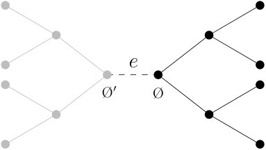 Figure 1
Peer Reviews
No public reviews on file for this paper yet. If you reviewed it on a platform where reviews are public (OpenReview, ICLR, NeurIPS, ICML), you can paste yours below so the community can read it here.
Videos
No videos yet. Explain this paper in a talk, walkthrough, or lecture? Add one.
A new upper bound for the critical probability of the frog model on homogeneous trees
Elcio Lebensztayn
Institute of Mathematics, Statistics and Scientific Computation
University of Campinas – UNICAMP
Rua Sérgio Buarque de Holanda 651, 13083-859, Campinas, SP, Brazil.
and
Jaime Utria
Abstract.
We consider the interacting particle system on the homogeneous tree of degree , known as frog model. In this model, active particles perform independent random walks, awakening all sleeping particles they encounter, and dying after a random number of jumps, with geometric distribution. We prove an upper bound for the critical parameter of survival of the model, which improves the previously known results. This upper bound was conjectured in a paper by Lebensztayn et al. (J. Stat. Phys., 119(1-2), 331–345, 2005). We also give a closed formula for the upper bound.
Key words and phrases:
Frog model, homogeneous tree, critical probability
2010 Mathematics Subject Classification:
60K35, 60J85, 82B26, 82B43
The authors were supported by the National Council for Scientific and Technological Development – CNPq.
1. Introduction
We study a system of branching random walks with random lifetime on a rooted graph, which is known as the frog model. This model is inspired by the process of an infection spreading (or rumor propagation) through a population, where the transmission agents are mobile particles which move along the vertices of the graph. Like the percolation model and other interacting particle systems such as the contact process, the frog model has two different types of behavior, depending on a parameter (, in this case). For small values of , the process dies out almost surely, whereas, for large , the process survives perpetually with positive probability. In this paper, we derive a new upper bound for the critical value that separates these two regimes for the model on homogeneous trees. This upper bound has been conjectured by Lebensztayn et al. [12]. For the proof, we construct an approximating sequence of processes that lead directly to the upper bound.
The frog model with geometric lifetime is defined as follows. Let be an infinite connected rooted graph. The root of is denoted by . We will assume that the system starts with one active particle located at , and one inactive particle at every other vertex of . Active particles perform independent simple random walks on , in discrete time, and have independent geometrically distributed random lifetimes, with parameter . That is, at each instant of time, every awake particle may disappear with probability ; if it survives, it moves to one of the neighboring vertices, chosen with uniform probability. Whenever an active particle hits a vertex containing a sleeping one, the latter is activated, and starts its own life and trajectory on , in an independent manner. We denote by the frog model on , with survival parameter , referring the reader to Alves et al. [1] for the formal definition of the model.
The question of phase transition for the frog model on infinite graphs was first addressed by Alves et al. [1], especially on the hypercubic lattices , , and homogeneous trees. Fontes et al. [5] prove that the critical probability is not a monotonic function of the underlying graph, which is an unexpected fact, as the frog model can be thought of as a percolation model. Lebensztayn and Utria [11] study the issue of phase transition on birregular trees. We present the known results regarding upper bounds for the critical parameter on homogeneous trees in Section 1.1.
For the frog model with , in which all awake frogs live perpetually, a fundamental problem is whether the root of the graph is visited by infinitely many frogs. In the first published paper dealing with the frog model, Telcs and Wormald [15] prove that this holds true almost surely on , for every , when the process starts with one particle per vertex. Popov [13] studies a phase transition from transience to recurrence, also on , with respect to the initial density of particles. The question of recurrence or transience for the frog model on integer lattices and infinite trees is an important topic of current research; see Döbler et al. [4], Hoffman et al. [8], Kosygina and Zerner [10], Rosenberg [14], and references therein. Other central problems for the model without death are related to the growth of the set of visited vertices, and the movement of the cloud of particles. We refer, for instance, to Alves et al. [2], Höfelsauer and Weidner [7], and Hoffman et al. [9].
1.1. Definitions and objectives
For , let denote the homogeneous tree of degree . We say that a particular realization of the frog model on survives if for every instant of time there is at least one awake particle. Otherwise, we say that it dies out. By a coupling argument, is a nondecreasing function of , and therefore we define the critical probability as
[TABLE]
As usual, we say that there is phase transition if . As proved by Alves et al. [1, Theorems 1.2 and 1.5], the frog model on with random initial configuration exhibits phase transition for every , under rather broad conditions.
The main result of Lebensztayn et al. [12, Theorem 4.1] states that, for the frog model on starting with one particle per vertex,
[TABLE]
In a remark at the end of Section 4 (p. 341), the authors claim that a refinement of the argument in the proof of (1.1) leads a better result, namely,
[TABLE]
where is the unique root in the interval of the quartic polynomial . However, as the authors point out, some technical difficulties prevent a full proof of (1.2). Our foremost purpose is to establish this new upper bound for , which also improves the result derived recently by Gallo and Rodríguez [6], using Renewal Theory. We present a proof of (1.2) that relies on the ideas of Lebensztayn et al. [12], but is completely independent, and has the advantage of offering a probabilistic interpretation, since it defines the approximation processes that allow us to arrive at formula (1.2).
2. Main results
For , we define
[TABLE]
where is the unique root in of the polynomial
[TABLE]
Let us denote by the upper bound for established in Gallo and Rodríguez [6, Proposition 2]:
[TABLE]
It is worth noting that this bound improves (1.1).
Theorem 2.1**.**
For every , we have that
- (i)
. 2. (ii)
* is the unique root in (0,1) of the polynomial*
[TABLE] 3. (iii)
.
For the sake of completeness, we write down an explicit formula for , not involving imaginary numbers. For this, we need the following definition.
Definition 2.1**.**
For every fixed , we define the constants
[TABLE]
Also, let
[TABLE]
Theorem 2.2**.**
For every ,
[TABLE]
3. Proof of Theorem 2.1
The key idea is to construct a class of Galton–Watson branching processes which are dominated by the frog model on , in the sense that the frog model survives if each one of these processes does. This approach is similar to that employed in Lebensztayn et al. [12] to prove (1.1). However, here the branching processes are defined in a new manner, in such a way that, by studying their critical behavior, we obtain directly a sequence of upper bounds for the critical probability, which converges to .
Let be fixed. The first step in the proof is to describe as a percolation model. Indeed, for each pair of distinct vertices of , we draw a directed edge from to if and only if the particle placed originally at ever visits the vertex , in the event of being activated. As usual, we denote this event by , and its complement by . Of course, the frog model survives if and only if there exists an infinite sequence of distinct vertices , satisfying (that is, the cluster of the root in the oriented percolation model has infinite size). As proved by Lebensztayn et al. [12, Lemma 2.1], the probability of is
[TABLE]
where is the distance between vertices and , and the function is given by
[TABLE]
We also recall from Lemma 3.1 of this paper that, for every ,
[TABLE]
In the sequel, we need the following definition.
Definition 3.1**.**
For , we define
[TABLE]
The central idea to prove Theorem 2.1 is summarized in the next result.
Lemma 3.1**.**
For every , there exist a Galton–Watson branching process embedded in , and a function (not depending on ) with domain , with the following properties:
- (i)
. 2. (ii)
The survival of implies the survival of the frog model on . 3. (iii)
The mean number of offspring per individual in equals
[TABLE]
Furthermore, for every ,
[TABLE]
Notice that, by finding such that each one of these branching processes is supercritical, we obtain a sequence of upper bounds for . Hence, to conclude that , it will suffice to show that converges to as . Before doing this, we present the construction of the branching processes and the proof of Lemma 3.1.
3.1. Proof of Lemma 3.1
To define the branching process , we consider the spreading of the frog model restricted to a tree rooted at , which is isomorphic to the -ary tree. First, given two vertices and of , we say that is a descendant of if is one of the vertices of the path connecting and . For , let denote the set consisting of all descendants of (including itself). Fixed an arbitrary vertex neighbor of the root, we define as the set of vertices in the subtree of rooted at , that is obtained by disconnecting from . See Figure 1. For a vertex and , we denote by the set of vertices in at distance from .
Definition 3.2**.**
For vertices and , let be the vertices in the path connecting and , in such a way that and are neighbors. For each , let denote the event that . Now we define the event inductively on by:
- (i)
If , then
[TABLE]
- (ii)
If , then
[TABLE]
- (iii)
If , then
[TABLE]
where
[TABLE]
Moreover, we denote the complement of by .
Fixed , let us define the Galton–Watson branching process embedded in . Consider , and, for , define
[TABLE]
Let denote the cardinality of . Thus, the process starts from the root of , and, given a vertex , its potential direct children are vertices located in . A vertex is regarded as a child of if and only if .
Notice that, for every , is indeed a branching process with , and whose survival implies the survival of the frog model on . To finish the proof of Lemma 3.1, we need to show part (iii) and formula (3.3). To this end, we define the sequence of functions with domain , inductively given by
[TABLE]
Then, part (iii) of Lemma 3.1 is established once we prove the following result.
Lemma 3.2**.**
For every , the probability of vertex being a child of is given by
[TABLE]
where is defined by (3.4).
Proof.
First, from (3.1), it follows that for all ,
[TABLE]
In addition, notice that can be obtained using the Inclusion-Exclusion Formula, and
[TABLE]
Hence, observing that for ,
[TABLE]
and using (3.1), the result follows by induction on . ∎
The proof of formula (3.3) proceeds in two steps, which are formulated in Lemmas 3.3 and 3.4.
Lemma 3.3**.**
The sequence satisfies the following linear difference equation of second order
[TABLE]
with initial conditions and
Proof.
It is straightforward to check that, for , both formulas (3.4) and (3.5) lead to . From (3.4), it follows that, for every ,
[TABLE]
as desired. ∎
Lemma 3.4**.**
For every , we have that
[TABLE]
Proof.
It is enough to consider . In order to solve (3.5), we compute the discriminant of the associated characteristic polynomial
[TABLE]
obtaining . Therefore, the equation (3.6) has two distinct real roots, which are given by
[TABLE]
The general solution of (3.5) is then expressed as
[TABLE]
where and are functions of , determined by the initial conditions. As , the result follows. ∎
Remark*.*
To derive a closed formula for , we can extend the sequence for the index , by rewriting
[TABLE]
with initial conditions and . By imposing these initial conditions in (3.7), we get
[TABLE]
Consequently, for every and ,
[TABLE]
We underline that equals the function obtained through the alternative method described by Lebensztayn et al. [12], in the remark at the end of Section 4, for constructing another approximating function to , such that for every . That is, is identical to the function that one obtains when the inequality for is used instead of for , in the definition of . This is the reason why the upper bound we establish here coincides with the one conjectured by Lebensztayn et al. [12].
3.2. Proof of Theorem 2.1
Again let be fixed. We define the functions
[TABLE]
From Equation (3.3), we have that, for every ,
[TABLE]
We also observe that
[TABLE]
where is the quartic polynomial given in (2.1). Since is an increasing function, satisfying and (as ), we conclude that the equivalent equations in (3.9) have a unique solution in the interval . In addition, from (3.2), it follows that
[TABLE]
is the unique root of the equation in the interval .
To prove part (i) of Theorem 2.1, we use the following fact of Real Analysis.
Lemma 3.5**.**
Let be a sequence of increasing, continuous real-valued functions defined on , such that and for every . Suppose that converges pointwise as to an increasing, continuous function defined on , and let be the unique root of in . Then, there exists and .
It is straightforward to check that and given in (3.8) satisfy the conditions of Lemma 3.5. Hence, by defining as the unique root of in the interval , we obtain that
[TABLE]
But for every , we have that , whence, from Lemma 3.1, the frog model on survives with positive probability. Consequently,
[TABLE]
and part (i) of Theorem 2.1 is established by taking .
Part (ii) is proved by expanding and simplifying properly the equation
[TABLE]
The formula manipulation involved can be accomplished by using a mathematical software. This tool can also be used to establish that for every . Together with the fact that , this yields part (iii). ∎
4. Proof of Theorem 2.2
In brief, the proof proceeds by using Descartes’ solution of a quartic equation and a couple of results to isolate the root in among the four roots of . The central steps are explained below. See Dickson [3] for an excellent account on the theory of equations.
First, notice that, by Descartes’ Rule of Signs, the polynomial given in (2.2) has either one or three positive roots. Naturally, is the smallest positive root. Using Descartes’ method, we apply the Tschirnhaus transformation to the equation , thereby obtaining the reduced form
[TABLE]
where and are given in Definition 2.1, and . Next we consider the auxiliary cubic equation
[TABLE]
To solve equation (4.1), we have to pick any nonzero root of (4.2), say , and define as either square root of the selected . Then, the four roots of (4.1) are the roots of the two quadratic polynomials
[TABLE]
which are given by
[TABLE]
To study the roots of (4.1), we compute the discriminant of the equation (4.2). This can be written as , where
[TABLE]
Notice that is a polynomial of degree . Using Budan–Fourier Theorem for and the fact that , we conclude that for , and for . Hence, we split the proof into two cases:
- (i)
: We have that , so the equation (4.1) has two distinct real and two imaginary roots, and therefore the roots of are one negative, one positive and two complex conjugate to each other. Moreover, the equation (4.2) has a unique real root, which is positive. The value of given in Definition 2.1 for equals the positive square root of this unique real root of equation (4.2), which is obtained using Cardano’s solution for cubic equations. We observe that and in (4.3) are imaginary numbers (otherwise would be negative). Consequently, is the unique positive root of . This completes the proof of the formula for in case (i). 2. (ii)
: As , and , the roots of (4.1) are all real and distinct, and this implies that has one negative and three positive roots. Furthermore, the equation (4.2) has three positive real roots, which are better expressed in a trigonometric form (the so-called irreducible case). The constant as given in Definition 2.1 for is the positive square root of one of these roots. Thus, the four roots of (4.1) are and . To finish the proof, it is enough to show that . But this inequality holds true, since . ∎
The reference list from the paper itself. Each links out to its DOI / PubMed record.
- 1Alves et al. [2002 a] O. S. M. Alves, F. P. Machado, and S. Popov. Phase transition for the frog model. Electron. J. Probab. , 7(16):21 pp., 2002 a.
- 2Alves et al. [2002 b] O. S. M. Alves, F. P. Machado, and S. Popov. The shape theorem for the frog model. Ann. Appl. Probab. , 12(2):534–547, 2002 b.
- 3Dickson [1914] L. E. Dickson. Elementary Theory of Equations . Cornell University Library historical math monographs. J. Wiley & Sons, New York, 1914.
- 4Döbler et al. [2018] C. Döbler, N. Gantert, T. Höfelsauer, S. Popov, and F. Weidner. Recurrence and transience of frogs with drift on ℤ d superscript ℤ 𝑑 \mathbb{Z}^{d} . Electron. J. Probab. , 23:23 pp., 2018.
- 5Fontes et al. [2004] L. R. Fontes, F. P. Machado, and A. Sarkar. The critical probability for the frog model is not a monotonic function of the graph. J. Appl. Probab. , 41(1):292–298, 2004.
- 6Gallo and Rodríguez [2018] S. Gallo and P. M. Rodríguez. Frog models on trees through renewal theory. J. Appl. Probab. , 55(3):887–899, 2018.
- 7Höfelsauer and Weidner [2016] T. Höfelsauer and F. Weidner. The speed of frogs with drift on ℤ ℤ \mathbb{Z} . Markov Process. Related Fields , 22(2):379–392, 2016.
- 8Hoffman et al. [2017] C. Hoffman, T. Johnson, and M. Junge. Recurrence and transience for the frog model on trees. Ann. Probab. , 45(5):2826–2854, 2017.