Simultaneous Confidence Bands for Functional Data Using the Gaussian Kinematic Formula
Fabian J.E. Telschow, Armin Schwartzman

TL;DR
This paper develops a method for constructing simultaneous confidence bands for functional data using the Gaussian Kinematic formula, demonstrating its effectiveness even with small samples and extending it to noisy, discretely sampled data.
Contribution
It introduces a CLT-based approach for applying the Gaussian Kinematic formula to non-Gaussian functional data, with practical extensions and a comprehensive simulation study.
Findings
tGKF performs well with small sample sizes
tGKF outperforms bootstrap methods for larger samples
Method is computationally efficient and applicable to DTI data
Abstract
This article constructs simultaneous confidence bands (SCBs) for functional parameters using the Gaussian Kinematic formula of -processes (tGKF). Although the tGKF relies on Gaussianity, we show that a central limit theorem (CLT) for the parameter of interest is enough to obtain asymptotically precise covering rates even for non-Gaussian processes. As a proof of concept we study the functional signal-plus-noise model and derive a CLT for an estimator of the Lipschitz-Killing curvatures, the only data dependent quantities in the tGKF SCBs. Extensions to discrete sampling with additive observation noise are discussed using scale space ideas from regression analysis. Here we provide sufficient conditions on the processes and kernels to obtain convergence of the functional scale space surface. The theoretical work is accompanied by a simulation study comparing different methods to…
Click any figure to enlarge with its caption.
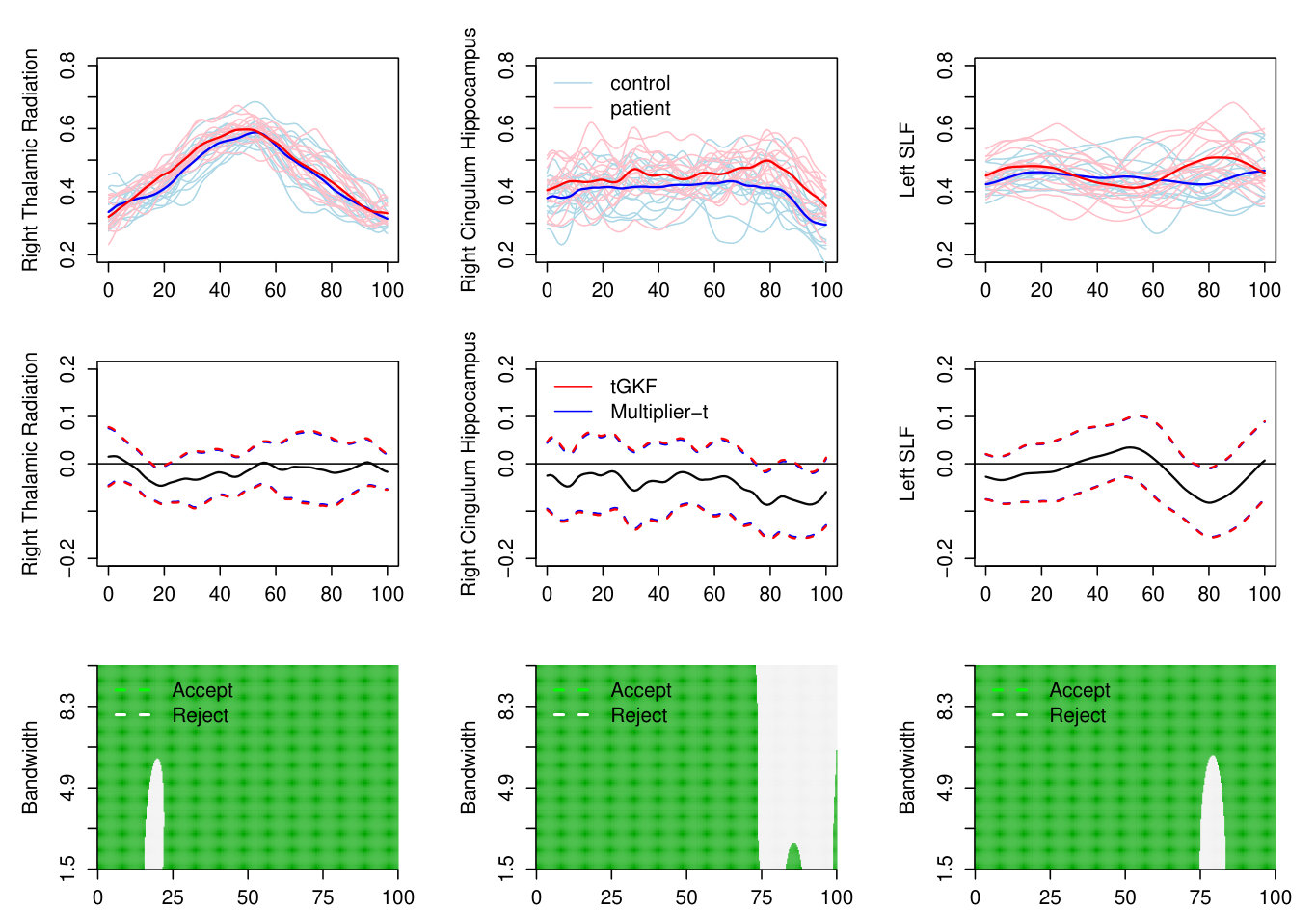 Figure 1
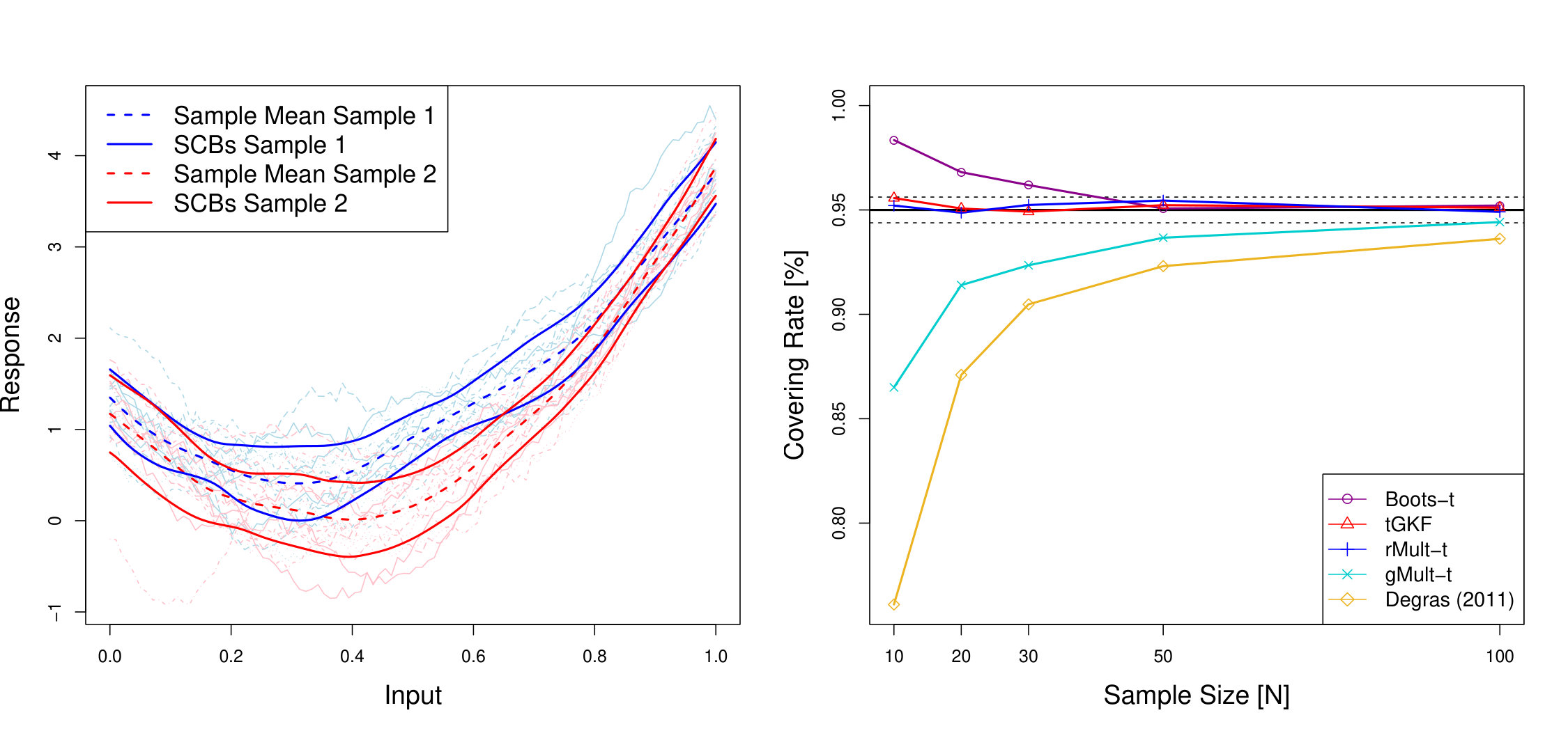 Figure 2
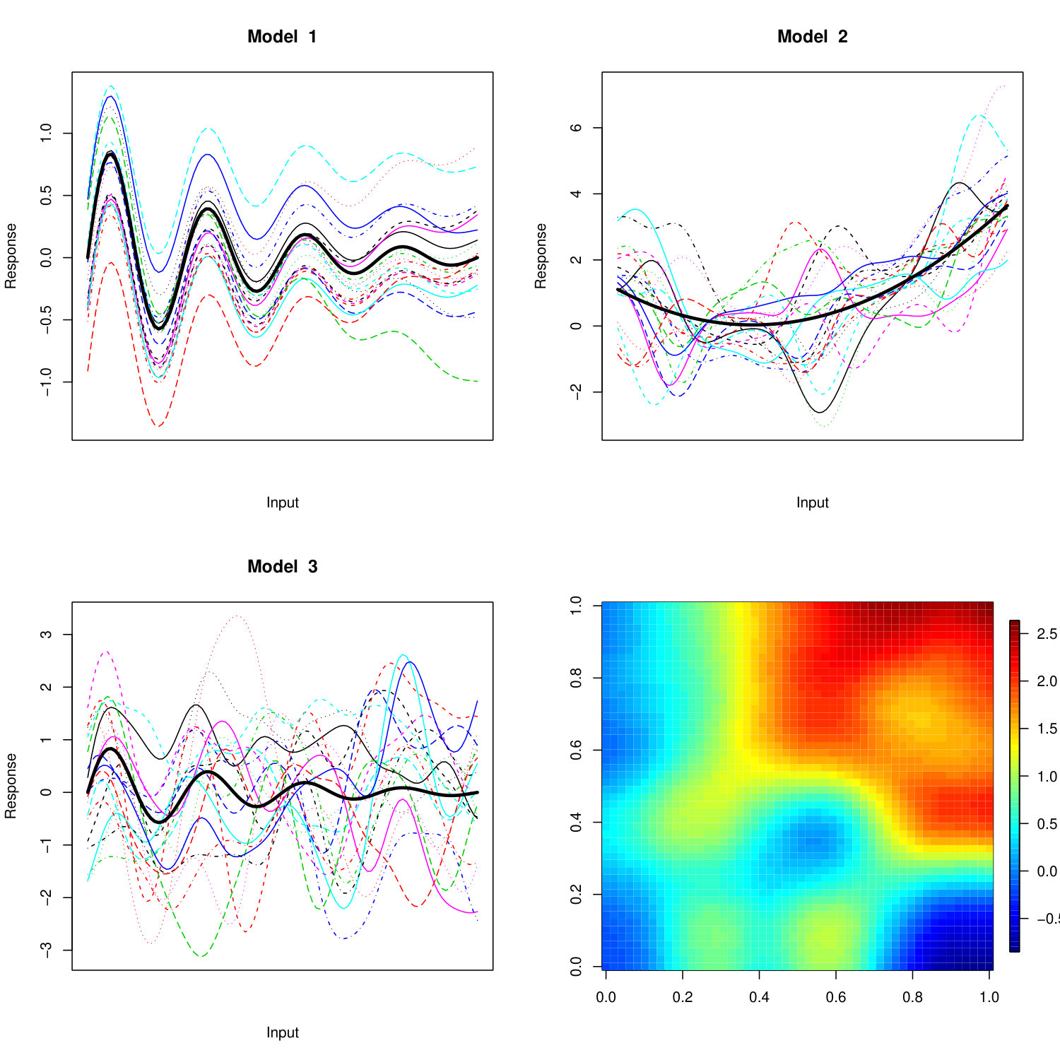 Figure 3
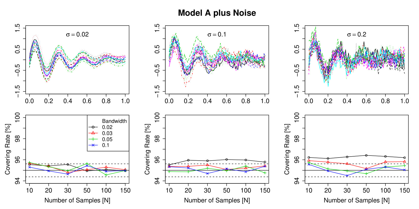 Figure 4
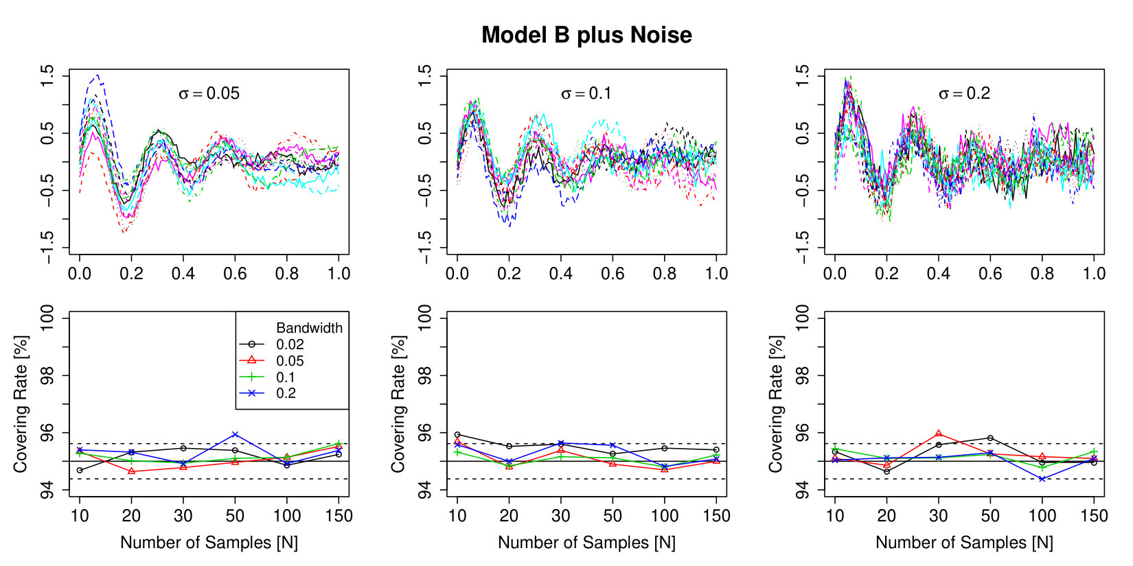 Figure 5
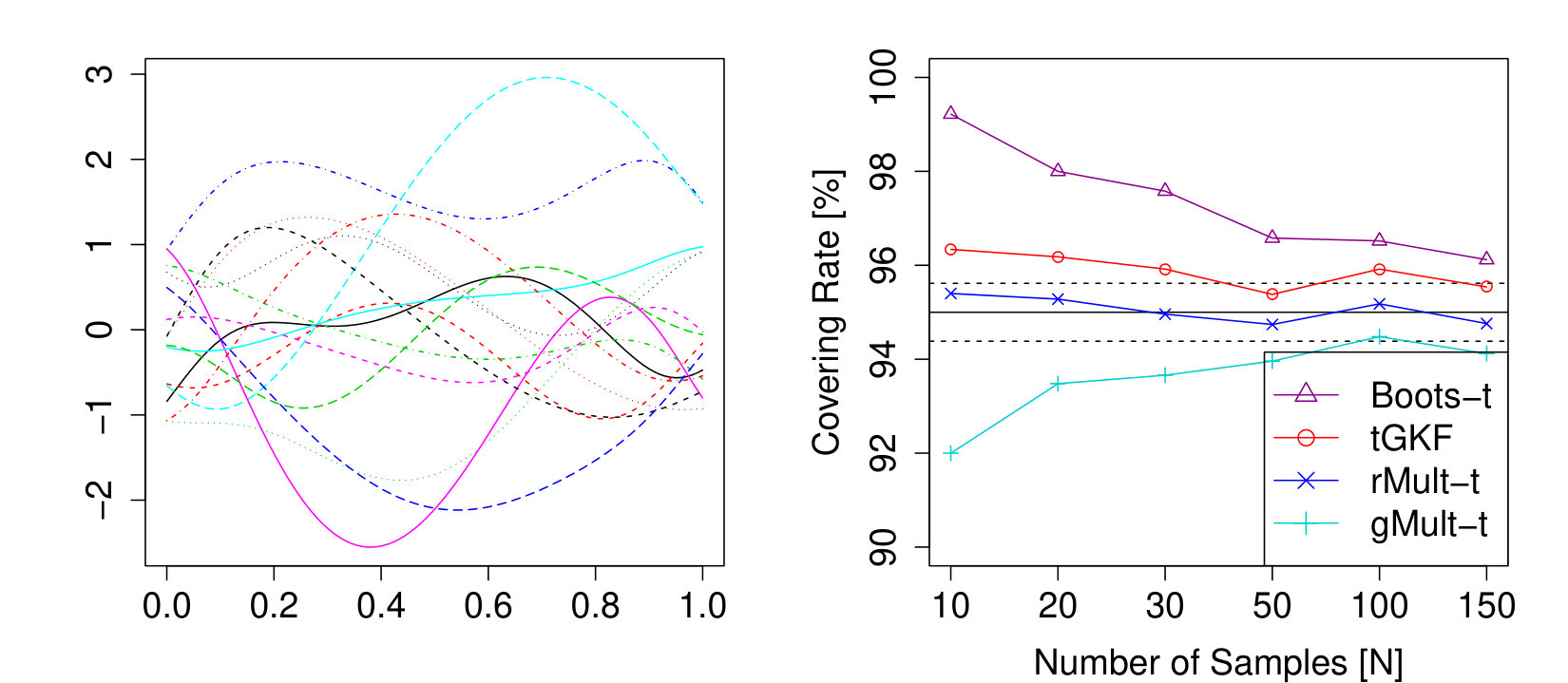 Figure 6
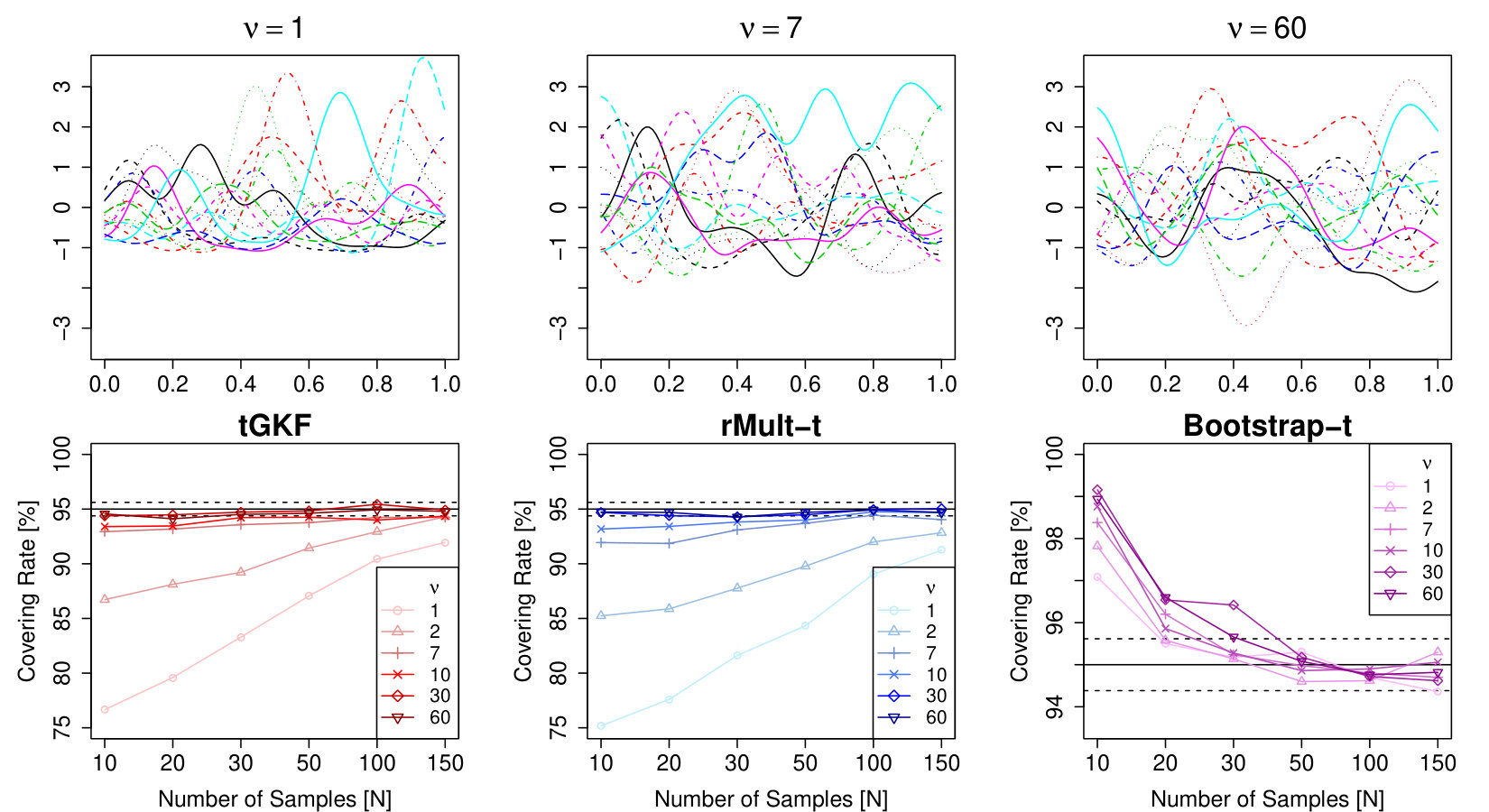 Figure 7
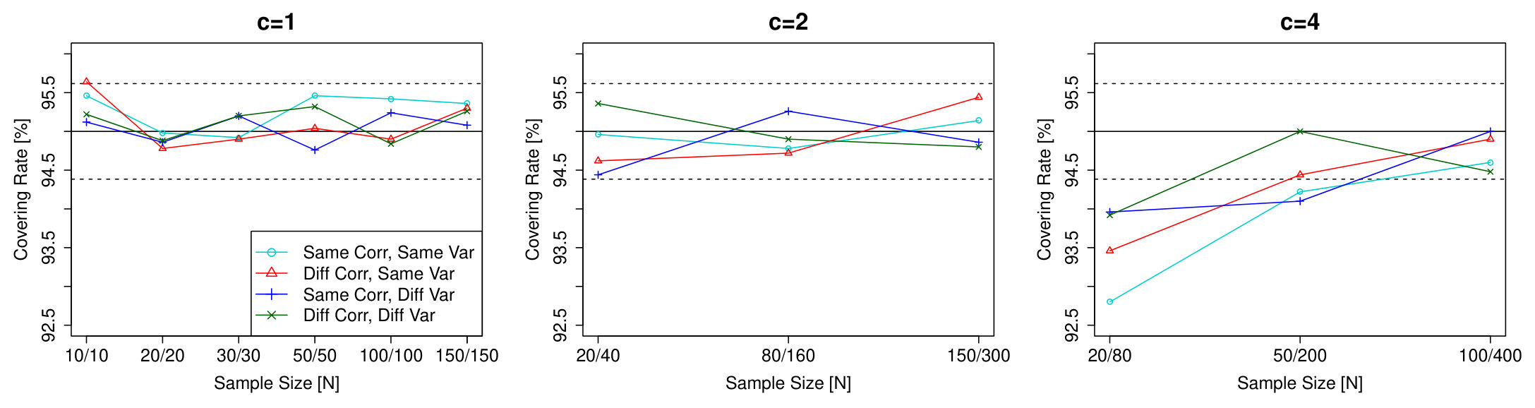 Figure 8
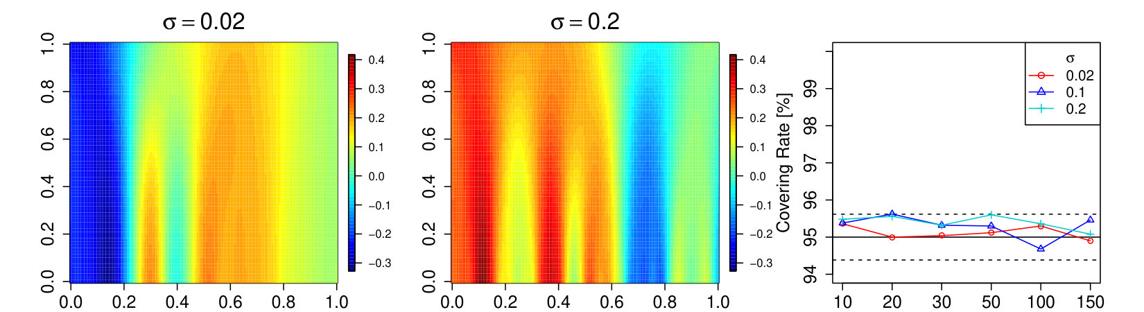 Figure 9
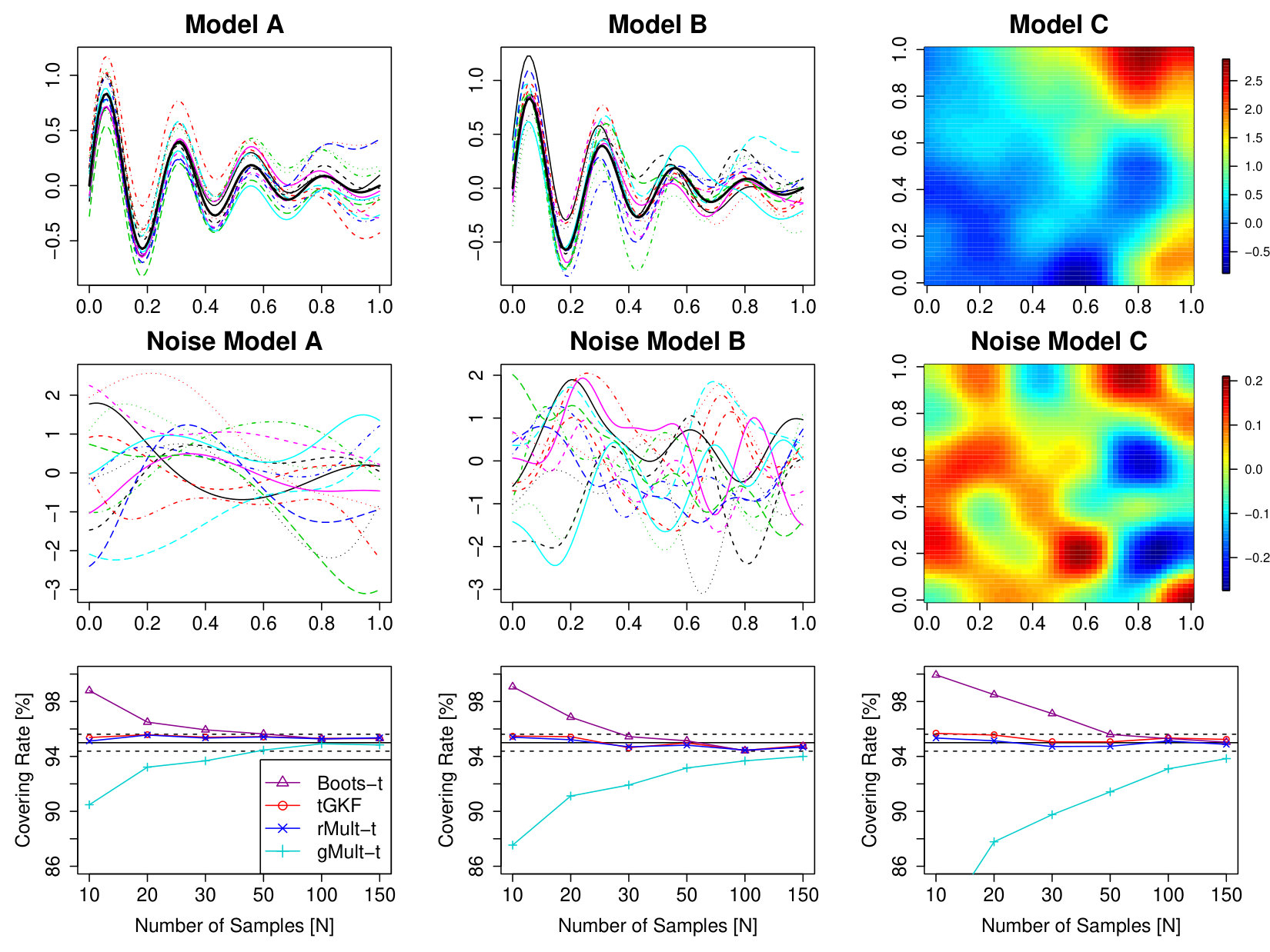 Figure 10
| N | ||||||
|---|---|---|---|---|---|---|
| true | 4.118 | 3.382 | 3.211 | 3.081 | 2.993 | 2.96 |
| tGKF | ||||||
| GKF | ||||||
| Degras | ||||||
| Boots | ||||||
| Boots-t | ||||||
| gMult | ||||||
| gMult-t | ||||||
| rMult | ||||||
| rMult-t |
| N | ||||||
|---|---|---|---|---|---|---|
| true | 4.532 | 3.628 | 3.373 | 3.19 | 3.048 | 3.004 |
| tGKF | ||||||
| GKF | ||||||
| Degras | ||||||
| Boots | ||||||
| Boots-t | ||||||
| gMult | ||||||
| gMult-t | ||||||
| rMult | ||||||
| rMult-t |
Peer Reviews
No public reviews on file for this paper yet. If you reviewed it on a platform where reviews are public (OpenReview, ICLR, NeurIPS, ICML), you can paste yours below so the community can read it here.
Videos
No videos yet. Explain this paper in a talk, walkthrough, or lecture? Add one.
Simultaneous Confidence Bands for Functional Data Using the Gaussian Kinematic Formula
Fabian J.E. Telschow, Armin Schwartzman
Abstract
This article constructs simultaneous confidence bands (SCBs) for functional parameters using the Gaussian Kinematic formula of -processes (tGKF). Although the tGKF relies on Gaussianity, we show that a central limit theorem (CLT) for the parameter of interest is enough to obtain asymptotically precise covering rates even for non-Gaussian processes. As a proof of concept we study the functional signal-plus-noise model and derive a CLT for an estimator of the Lipschitz-Killing curvatures, the only data dependent quantities in the tGKF SCBs. Extensions to discrete sampling with additive observation noise are discussed using scale space ideas from regression analysis. Here we provide sufficient conditions on the processes and kernels to obtain convergence of the functional scale space surface.
The theoretical work is accompanied by a simulation study comparing different methods to construct SCBs for the population mean. We show that the tGKF works well even for small sample sizes and only a Rademacher multiplier- bootstrap performs similarily well. For larger sample sizes the tGKF often outperforms the bootstrap methods and is computational faster. We apply the method to diffusion tensor imaging (DTI) fibers using a scale space approach for the difference of population means. R code is available in our Rpackage SCBfda.
Contents
1 Introduction
In the past three decades functional data analysis has received increasing interest due to the possibility of recording and storing data collected with high frequency and/or high resolution in time and space. Many different methods have been developed to study these particular data objects; for overviews of some recent developments in this fast growing field we refer the reader to the review articles Cuevas, (2014) and Wang et al., (2016).
Currently, the literature on construction of simultaneous confidence bands (SCBs) for functional parameters derived from repeated observations of functional processes is sparse. The existing methods basically split into two seperate groups. The first group is based on functional central limit theorems (fCLTs) in the Banach space of continuous functions endowed with the maximum metric and evaluation of the maximum of the limiting Gaussian process often using Monte-Carlo simulations with an estimated covariance structure of the limit process, cf. Bunea et al., (2011); Degras, (2011, 2017); Cao et al., (2012, 2014). The second group is based on the bootstrap, among others Cuevas et al., (2006); Chernozhukov et al., (2013); Chang et al., (2017), Belloni et al., (2018).
Although these methods are asymptotically achieving the correct covering probabilities, their small sample performance is often less impressive as for example discovered in Cuevas et al., (2006). Figure 1 shows the typical behaviour observed in our simulations of the covering rates of SCBs for the (smoothed) population mean using replications of a (smoothed) Gaussian process with an unknown non-isotropic covariance function. The general pattern is that SCBs using a non-parametric bootstrap- yield too wide confidence bands and thus have overcoverage, whereas a functional Gaussian multiplier bootstrap inspired by Chernozhukov et al., (2013) and Degras, (2011) asymptotic SCBs lead to undercoverage. We used here SCBs for the smoothed population mean, since the R-package SCBmeanfd by Degras does require smoothing.
Contrary to most of the current methods, which assume that each functional process is observed only at discrete points of their domain, we start from the viewpoint that the whole functional processes are observed and sufficiently smooth, since often the first step in data analysis is anyhow smoothing the raw data. This implies that we construct SCBs only for the smoothed population parameter and thereby circumventing the bias problem altogether to isolate the covering aspect. In principle, however, it is possible to apply our proposed method also to discretely observed data and inference on the true (non-smoothed) mean as for example in settings described in Zhang et al., (2007); Degras, (2011); Zhang et al., (2016). But for the sake of simplicity we restrict ourselves to only robustify against the choice of a smoothing parameter by introducing SCBs for scale space surfaces, which were proposed in Chaudhuri and Marron, (1999).
The main contribution of this paper is proposing the construction of SCBs for general functional parameters based on the Gaussian kinematic formula for -processes (tGKF) and studying its theoretical covering properties. Moreover, as an important case study we explain and prove how all the required assumptions can be satisfied for construction of SCBs for the population mean in functional signal-plus-noise models and scale spaces. A first glance on the improvement, especially for small samples, using the tGKF is shown in Figure 1.
A second contribution is that we compare to a studentized version of the multiplier bootstrap based on residuals, which we call multiplier- bootstrap (Mult-), which also improves the small sample properties of the bootstrap SCBs considerably, if the multiplier is chosen to be Rademacher random variables. Since the scope of the paper is to analyse the theoretical properties of the use of the tGKF in construction of SCBs, we do not provide any rigorous mathematical theory about the Mult- bootstrap. Theoretical analysis of this bootstrap method, in particular the influence of the choice of multiplier, is an interesting opportunity for future research. For recent work on the performance of different multipliers in similar scenarios, see e.g., Deng and Zhang, (2017) and Davidson and Flachaire, (2008).
SCBs usually require estimation of the quantiles of the maximum of a process. Often this process is the maximum of a process derived from a functional central limit theorem (fCLT); thus the maximum of a Gaussian process. Our proposed method tries to resolve the poor covering rates for small sample sizes by imposing two small but significant changes. Firstly, we use a pointwise -statistic, since for small sample sizes and unknown variance this would be the best choice to construct confidence bands for Gaussian random variables. Secondly, we employ a formula which is known to approximate the tail distribution of the maximum of a pointwise -distributed process very well. This formula is known as the Gaussian kinematic Formula for -processes (tGKF).
In a nutshell the tGKF as proven in even more generality in Taylor, (2006) expresses the expected Euler characteristic (EEC) of the excursion set of a random process , , derived from unit variance Gaussian processes indexed by a nice compact subset of in terms of a finite sum of known functions with corresponding coefficients. These coefficients are called Lipschitz-Killing curvatures (LKCs) and depend solely on the random process . Earlier versions of this formula derived in Adler, (1981) for Gaussian processes were used by Worsley et al., (1996),Worsley et al., (2004) in neuroscience for multiple testing corrections. Takemura and Kuriki, (2002) have shown that the GKF (for Gaussian processes) is closely related to the Volume of Tubes formula dating all the way back to Working and Hotelling, (1929) and which has been applied for SCBs in nonlinear regression analysis, e.g., Johansen and Johnstone, (1990); Krivobokova et al., (2010); Lu and Kuriki, (2017).
In this sense the version of the tGKF of Taylor, (2006) can be interpreted as a generalization of the volume of tube formula for repeated observations of functional data. The most important and valuable aspect of the tGKF is that it is a non-asymptotic formula in the sample size . Hence it is suitable for applications with small sample sizes. Moreover, it has been proven in Taylor et al., (2005) that the EEC is a good approximation of the quantile of the maximum value of Gaussian- and -processs over their domain. Although it is not yet proven, simulations suggest that this property seems to be also true for more complicated Gaussian related processes like -processes. Therefore, it can be used to control the family wise error rate (FWER) as in Taylor and Worsley, (2007); Taylor et al., (2009). To the best of our knowledge, the full potential of the tGKF for functional data seems to not have been explored yet in the statistical literature and we will try to fill this gap and tie together some loose strings for the challenge of constructing SCBs.
Our main theoretical contributions are the following. In Theorem 2 we show based on the main result in Taylor et al., (2005) that asymptotically the error in the covering rate of SCBs for a function-valued population parameter based on the GKF for -processes can be bounded and is small, if the targeted covering probability of the SCB is sufficiently high. This requires no Gaussianity of the observed processes. It only requires that the estimator of the targeted function-valued parameter fulfills a fCLT in the Banach space of continuous functions with a sufficiently regular Gaussian limit process. Moreover, it requires consistent estimators for the LKCs. Using this general result we derive SCBs for the population mean and the difference of population means for functional signal-plus-noise models, where we allow the error processes to be non-Gaussian. Especially we derive for such models defined over sufficiently regular domains , , consistent estimators for the LKCs. These estimators are closely related to the discrete estimators in Taylor and Worsley, (2007), but we can even prove CLTs for our estimators. In order to deal with observation noise we give in Theorem 8 sufficient conditions to have weak convergence of a scale space process to a Gaussian limit extending the results from Chaudhuri and Marron, (2000) from regression analysis to repeated observations of functional data. Additionally, we prove that also the LKCs of this limit process can be consistently estimated and therefore Theorem 2 can be used to bound the error in the covering rate for SCBs of the population mean of a scale space process.
These theoretical findings are accompanied by a simulation study using our Rpackage SCBfda, which can be found on https://github.com/ftelschow/SCBfda and a data application to diffusion tensor imaging (DTI) fibers using a scale space approach for the difference of population means. In the simulation study we compare the performance of the tGKF approach to SCBs for different error processes mainly with bootstrap approaches and conclude that the tGKF approach does not only often give better coverings for small sample sizes, but also outperforms bootstrap approaches computationally. Moreover, the average width of the tGKF confidence bands is lower for large sample sizes.
Organisation of the Article
Our article is organized as follows: In Section 2.1 we describe the general idea of construction of SCBs for functional parameters. Section 2.2 defines the functional signal-plus-noise model and general properties on the error processes, which are necessary to prove most of our theorems. The next section explains how SCBs can be constructed in praxis and especially explains how the tGKF can be used for this purpose. Section 4 finally proves asymptotic properties of the SCBs constructed using the tGKF for general functional parameters. The latter require consistent estimation of the LKCs, which are discussed for the functional signal-plus-noise model in Section 5 together with the new CLTs for the LKCs. Robustification using SCBs for Scale Space models can be found in 6. In Section 7 we compare our proposed method in different simulations to competing methods to construct SCBs in the case of the functional signal-plus-noise model for various settings, which is followed in Section 8 by a data example.
2 Simultaneous Confidence Bands
2.1 SCBs for Functional Parameters
We describe now a general scheme for construction of simultaneous confidence bands (SCBs) for a functional parameter , , where is a compact metric space. Note that all functions of hereafter will be assumed to belong to the space of continuous functions from to .
Assume we have estimators of and estimating a different functional parameter fulfilling
[TABLE]
Here and whenever convergence of random continuous functions is considered, “” denotes weak convergence in endowed with the maximums norm . In (E1), is a mean zero Gaussian process with covariance function satisfying for all , is a scaling sequence of positive numbers. Assumptions (E1) and (E2) together with the functional version of Slutzky’s Lemma imply
[TABLE]
Thus, it is easy to check that the collection of intervals
[TABLE]
form -simultaneous confidence bands of , i.e.
[TABLE]
provided that
[TABLE]
Unfortunately, the quantiles are in general unknown and need to be estimated. Therefore, the main contribution of this article is the study and comparison of different estimators for .
In principle, there are two general approaches. Limit approximations try to estimate by approximations of the quantiles of the asymptotic process, i.e.
[TABLE]
as done in Degras, (2011, 2017) for the special case of a signal-plus-noise model and the local linear estimator of the signal. Here usually the covariance function is estimated and then many samples of the Gaussian process are simulated in order to approximate .
Better performance for finite sample sizes can be achieved by approximating directly by bootstrap approaches such as a fully non-parametric bootstrap proposed in Degras, (2011), which is inspired by the bootstrap- confidence intervals (e.g., DiCiccio and Efron, (1996)),.
Moreover, the tGKF approach, which we will introduce in Section 3.1, uses a “parametric” estimator of , approximating the l.h.s of (1) by a -process over .
2.2 Functional Signal-Plus-Noise Model
Our leading example will be SCBs for the population mean curve in a functional signal-plus-noise model which we will introduce now. Let us assume that , , is a compact set with piecewise -boundary . The functional signal-plus-noise model is given by
[TABLE]
Here we assume that are continously differentiable functions on and is a stochastic process with zero mean and covariance function for satisfying if and only if . Moreover, we introduce the following useful properties of stochastic processes.
Definition 1**.**
We say a stochastic process with domain is Lipschitz, if there is a (semi)-metric on continuous w.r.t. the standard metric on and a random variable satisfying \mathbb{E}\big{[}|A|^{p}\big{]}<\infty such that
[TABLE]
and , where denotes the metric entropy function of the (semi)-metric space , e.g., Adler and Taylor, (2007, Def. 1.3.1.).
Remark 1**.**
Any Lipschitz process has necessarily almost surely continuous sample paths. Moreover, this property is the main ingredient in the version of a CLT in proven in Jain and Marcus, (1975) or Ledoux and Talagrand, (2013, Section 10.1). However, there are different results on CLTs in with different assumptions on the process, which in principle could replace this condition. For example for we could also use the condition
[TABLE]
where is non-decreasing near 0 and satisfies . This is due to Hahn, (1977). However, -Lipschitz seems to be the most tractable assumption for our purposes.
Definition 2**.**
We say a process has finite -th -moment, if \mathbb{E}\big{[}\|Z(s)\|^{p}_{\infty}\big{]}<\infty.
Proposition 1**.**
Any Lipschitz process over a compact set has finite -th -moment.
Remark 2**.**
Since any continuous Gaussian process satisfies the finite -th -moment condition, cf. Landau and Shepp, (1970), it is possible to proof a reverse of Proposition 1 for continuously differentiable Gaussian processes. Moreover, finite -th -moment conditions are often assumed, when uniform consistency of estimates of the covariance function are required, e.g., Hall et al., (2006) and Li et al., (2010).
3 Estimation of the Quantile
This section describes different estimators for the quantiles defined by equation (3). Especially, we propose using the Gaussian kinematic formula for -processes (tGKF) as proven in Taylor, (2006). Moreover, we describe different bootstrap estimators.
3.1 Estimation of the Quantile Using the tGKF
3.1.1 The Gaussian Kinematic Formula for t-processes
A -process over an index set is a stochastic process such that is -distributed for all . In order to match the setting in Taylor, (2006) we assume that the process is given by
[TABLE]
where are mean zero, variance one Gaussian processes. Let us define , where denotes the number of elements in the multi-index . Then we require the following assumptions:
- (G1)
has almost surely sample paths. 2. (G2)
The joint distribution of \Big{(}D^{d}\mathcal{G}(s),D^{(d,l)}\mathcal{G}(s)\Big{)} is nondegenerate for all and . 3. (G3)
There is an such that
[TABLE]
for all and for all . Here and are finite constants.
Remark 3**.**
Assumption (G3) is satisfied for any process having almost surely sample paths and all third derivatives have finite second -moment, see Definiton 2. In particular, this holds true for any Gaussian process with sample paths. For completeness the argument is carried out in more detail in the appendix.
Under these assumptions the tGKF is an exact, analytical formula of the expectation of the Euler characteristic of the excursion sets of . This formula as proven in Taylor, (2006) or Adler and Taylor, (2007) is
[TABLE]
where , , is the -th Euler characteristic density of a -process, which can be found for example in Taylor and Worsley, (2007). Moreover, denotes the -th Lipschitz killing curvature, which only depends on and the parameter space . Note that .
Equation (8) is useful, since by the expected Euler characteristic heuristic (EECH) (see Taylor et al., (2005) ), we expect
[TABLE]
to be a good approximation for large thresholds . In the case that this approximation actually is always from above. This is due to the fact that the Euler characteristic of one-dimensional sets is always non-negative and hence using the Markov-inequality we obtain
[TABLE]
The same argument is heuristically valid for high enough thresholds in any dimension, since the excursion set will with high probabilty consist mostly of simply-connected sets. Thus, the EC of the excursion set will be positive with high probability. Therefore, once again we expect that the EEC is an approximation from above for the excursion probability.
Notably, the tGKF Equation (8) had a predecessor for the EEC of a Gaussian processes . Remarkably, the only difference between these formulas is that the Euler characteristic densities are different, see Adler and Taylor, (2007, p.315, (12.4.2)). Moreover, the approximation error when using the EEC instead of the excursion probabilities of the Gaussian process has been analytically quantified in Taylor et al., (2005).
3.1.2 The tGKF-estimator of
Assume that we have consistent estimators for the LKCs for all (we provide such estimators for in Section 5). Then a natural estimator of the quantile is the largest solution of
[TABLE]
The following result will be used in the next section for the proof of the accuracy of the SCBs derived using the tGKF estimator .
Theorem 1**.**
Assume that is a consistent estimator of . Then given by (11) converges almost surely for tending to infinity to the largest solution of
[TABLE]
where are the Euler characteristic densities of a Gaussian process, which can be found in Adler and Taylor, (2007, p.315, (12.4.2)).
3.2 Estimation of the Quantile Using the Bootstrap
As alternatives to the approach using the tGKF we discuss a non-parametric bootstrap- and a multiplier bootstrap estimator of the quantile defined in Equation (3).
3.2.1 Non-parametric bootstrap-
Based on Degras, (2011) we review a bootstrap estimator of the quantile . Assume that the estimators and are obtained from a sample of random functions, then the non-parametric bootstrap- estimator of is obtained as follows
Resample from with replacement to produce a bootstrap sample . 2. 2.
Compute and using the sample . 3. 3.
Compute T^{*}=\max_{s\in\mathcal{S}}\tau_{N}\big{|}\hat{\eta}^{*}_{N}(s)-\hat{\eta}_{N}(s)\big{|}/\hat{\varsigma}_{N}^{*}(s). 4. 4.
Repeat steps 1 to 3 many times to approximate the conditional law \mathcal{L}^{*}=\mathcal{L}\big{(}T^{*}\,|\leavevmode\nobreak\ Y_{1},...,Y_{N}\big{)} and take the quantile of to estimate .
Remark 4**.**
Note that the variance in the denominator is also bootstrapped, which corresponds to the standard bootstrap- approach for confidence intervals, cf. DiCiccio and Efron, (1996). This is done in order to mimic the l.h.s. in (1), and improves the small sample coverage. Results of this bootstrap variant will be discussed in our simulations.
We expect that this estimator works well for large enough sample sizes. Although Degras, (2011) introduced it especially for small sample sizes, there is not much hope that it will perform well in this case, since it is well known that confidence bands for a finite dimensional parameter based on the bootstrap- have highly variable end points, cf., Good, (2005, Section 3.3.3). Evidence that this remains the case in the functional world will be given in our simulations in Section 7.
3.2.2 Multiplier- Bootstrap
The second bootstrap method, which we introduce, builds on residuals and a version of the multiplier (or Wild) bootstrap (e.g., Mammen, (1993)) designed for the maximum of sums of independent random variables in high dimensions as discussed in detail by Chernozhukov et al., (2013). Briefly, the approach in Chernozhukov et al., (2013) is as follows. Let be independent random vectors in , with \mathbb{E}\big{[}X_{n}\big{]}=0 and finite covariance \mathbb{E}\big{[}X_{n}X_{n}^{T}\big{]} for all . Define X_{n}^{T}=\big{(}X_{n1},...,X_{nK}\big{)} and assume there are such that c<\mathbb{E}\big{[}X_{nk}^{2}\big{]}<C for all and all . Under these assumptions it is shown in Chernozhukov et al., (2013, Theorem 3.1) that the quantiles of the distribution of
[TABLE]
can be asymptotically consistently estimated by the quantiles of the multiplier bootstrap i.e., by the distribution of
[TABLE]
with multipliers given the data , even if .
We adapt this approach to the estimation of for functional parameters. Therefore we again assume that the estimators and are obtained from an i.i.d. sample of random functions. However, here we also need to assume that we have residuals for satisfying and mutual independence for tending to infinity. For example for the signal-plus-noise model, where and are the pointwise sample mean and the pointwise sample standard deviation, the residuals do satisfy these conditions, if the error process is -Lipschitz and has finite second -moment. Thus, using these assumptions we obtain that
[TABLE]
have approximately the same distribution. Algorithmitically, our proposed multiplier bootstrap is
Compute residuals and multipliers with and 2. 2.
Estimate from . 3. 3.
Compute . 4. 4.
Repeat steps 1 to 3 many times to approximate the conditional law \mathcal{L}^{*}=\mathcal{L}\big{(}T^{*}\,|\leavevmode\nobreak\ Y_{1},...,Y_{N}\big{)} and take the quantile of to estimate .
In our simulations we use Gaussian multipliers as proposed in Chernozhukov et al., (2013), but find that Rademacher multipliers as used in regression models with heteroskedastic noise, e.g. Davidson and Flachaire, (2008), perform much better for small sample sizes.
Remark 5**.**
Again the choice to compute bootstrapped versions of mimics the true distribution of the maximum of the random process on the l.h.s of (1) for finite better than just applying the multipliers to .
4 Asymptotic Covering Rates
4.1 Asymptotic SCBs for Functional Parameters
This section discusses the accuracy of the SCBs derived using the tGKF. Since the expected Euler characteristic of the excursion sets are only approximations of the excursion probabilities, there is no hope to prove that the covering of these confidence bands is exact. Especially, if is large the approximation fails badly and will usually lead to confidence bands that are too wide. However, for values of typically used for confidence bands, the EEC approximation works astonishingly well. Theoretically, this has been made precise for Gaussian processes in Theorem 4.3 of Taylor et al., (2005), which is the main ingredient in the proof of the next result. Additionally, it relies on the fCLT (1) and the consistency of for proved in Theorem 1.
Theorem 2**.**
Assume (E1-2) and assume that the limiting Gaussian process satisfies (G1-3). Moreover, let be a sequence of consistent estimators of for . Then there exists an such that for all we have that the SCBs defined in Equation (2) fullfill
[TABLE]
where is the critical variance of an associated process of , is the quantile estimated using equation (11) and is defined in Theorem 1.
Typically, in our simulations we have that, for , the quantile is about leading to an upper bound of , if we use the weaker bound without the critical variance.
4.2 Asymptotic SCBs for the Signal-Plus-Noise Model
As an immediate application of Theorem 2 we derive now SCBs for the population mean and the difference of population means in one and two sample scenarios of the signal-plus-noise model introduced in Section 2.2. The derivation of consistent estimators for the LKCs will be postponed to the next section.
Theorem 3** (Asymptotic SCBs for Signal-Plus-Noise Model).**
Let be a sample of model (5) and assume is an Lipschitz process. Define \textbf{Y}(s)=\big{(}Y_{1}(s),...,Y_{N}(s)\big{)}.
- (i)
Then the estimators
[TABLE]
fullfill the conditions (E1-2) with , , and . 2. (ii)
*If there are consistent estimators of the LKCs and has -sample paths and all partial derivatives up to order of are *Lipschitz processes with finite -variances and fullfills the non-degeneracy condition (G2), then the accuracy result of Theorem 2 holds true for the SCBs
[TABLE]
with of Theorem 1.
Remark 6**.**
A simple condition on to ensure that fulfills the non-degeneracy condition (G2) is that for all we have that has full rank for all . A proof is provided in Lemma 5 in the appendix.
Theorem 4** (Asymptotic SCBs for Difference of Means of Two Signal-Plus-Noise Models).**
Let and be independent samples, where
[TABLE]
with both Lipschitz processes and assume that . Then
- (i)
Condition (E1) is satisfied, i.e.
[TABLE]
where are Gaussian processes with the same covariance structures as and and the denominator converges uniformly almost surely, i.e. condition (E2) is satisfied. 2. (ii)
*If there are consistent estimators of the LKCs of and have -sample paths, fullfill the non-degeneracy condition (G2) and all their partial derivatives are *Lipschitz processes with finite -variances, then the accuracy result of Theorem 2 holds true for the SCBs
[TABLE]
with of Theorem 1.
5 Estimation of the LKCs for Signal-Plus-Noise Models
We turn now to consistent estimators of the LKCs. However, we treat only the case where is a process defined over a domain , where is assumed to be either a compact collection of intervals in or a compact two-dimensional domain of with a piecewise -boundary . We restrict ourselves to this setting, since there are simple, explicit formulas for the LKCs.
5.1 Definition of the LKCs for and
The basic idea behind the Lipschitz-Killing curvatures is that they are the intrinsic volumes of with respect to the pseudo-metric which is induced by the pseudo Riemannian metric given in standard coordinates of , cf. Taylor and Adler, (2003),
[TABLE]
For the cases the general expressions from Adler and Taylor, (2007) can be nicely simplified. For , i.e. , the only unknown is , which is given by
[TABLE]
In the case of with piecewise -boundary parametrized by the piecewise -function the LKCs are given by
[TABLE]
Note that by the invariance of the length of a curve the particular choice of the parametrization of does not change the value of .
5.2 Simple Estimators Based on Residuals
In order to estimate the unknown LKCs and from a sample of model (5), we assume that the estimators of and of satisfy (E1-2) with and
- (L)
for all almost surely.
These conditions imply that the normed residuals
[TABLE]
and its gradient converge uniformly almost surely to the random processes and . Let us denote the vector of residuals by \textbf{R}(s)=\big{(}R_{1}(s),...,R_{N}(s)\big{)}. In view of equation (16) it is hence natural to estimate the LKC for by
[TABLE]
and using equations (17) the LKCs for by
[TABLE]
where is the empirical covariance matrix of . Thus, we need to study mainly the properties of this estimator to ensure properties of the estimated LKCs.
Theorem 5**.**
Assume and for are Lipschitz processes and (E2) and (L) hold true. Then, we obtain
[TABLE]
If and for are even Lipschitz processes, we obtain
[TABLE]
with mapping
[TABLE]
and the matrix valued covariance function is given componentwise by
[TABLE]
for all and .
From this theorem we can draw two interesting results for . The first one is a consistency results of the LKCs. In a sense this is just reproving the result for the discrete estimator given in Taylor and Worsley, (2007) without the need to refer to convergences of meshes and making underlying assumptions more visible. Especially, it becomes obvious that the Gaussianity assumption on is not required, since we only have to estimate the covariance matrix of the gradient consistently.
Theorem 6** (Consistency of LKCs).**
Under the setting of Theorem 5 it follows for that
[TABLE]
An immediate corollary can be drawn for the generic pointwise estimators in the functional signal-plus-noise Model.
Corollary 1**.**
Let and assume that and for are Lipschitz processes. Then for we obtain
[TABLE]
Remark 7**.**
If the process is Gaussian then we can even infer that the estimators (19) and (20) are unbiased, if , see Taylor and Worsley, (2007).
The second conclusion we can draw from this approach is that we can derive a CLT for the estimator of the LKCs.
Theorem 7** (CLT for LKCs).**
Assume and for are even Lipschitz processes and (E2) and (L) hold true. Then, if ,
[TABLE]
and, if , we obtain
[TABLE]
where is a Gaussian process with mean zero and covariance function as in Theorem 5 and is a parametrization of the boundary .
Corollary 2**.**
Assume additionally to the Assumptions of Theorem 7 that is Gaussian with covariance function and . Then, we have the simplified representation
[TABLE]
where
[TABLE]
5.3 Estimation of LKCs in the Two Sample Problem
In the previous section we dealt with the case of estimating the LKCs in the case of one sample. This idea can be extended to the two sample case leading to a consistent estimator of the LKCs of the asymptotic process given in Theorem 4. Using the same notations as before we have that the difference in mean satisfies the following fCLT
[TABLE]
Therefore, note that independence of the samples implies that the covariance matrix defined in equation (15) splits into a sum of covariance matrices depeding on and , i.e.,
[TABLE]
The latter summands, however, under the assumptions of Theorem 5 can be separately consistently estimated using the previously discussed method and the residuals
[TABLE]
The sum of these estimators is a consistent estimator of and thus the estimator described in the previous section based on the estimate of using the above residuals gives a consistent estimator of the LKCs of .
6 Discrete Measurements, Observation Noise and Scale Spaces
We discuss now the realistic scenario, where the data is observed on a measurement grid with possible additive measurement noise. Again for simplicity we restrict ourselves to the signal-plus-noise model, which is
[TABLE]
where . Here we assume that is stochastic process on with finite second -moment representing the observation noise and covariance function . We also assume that , and are mutually independent. We are interested in doing inference on the mean , if we observe a sample .
Since it is still a challenge to optimally choose the bandwidth for finite and especially small sample sizes, if we want to estimate the population mean directly, we rather rely here on the idea of scale spaces, which was originally introduced for regression in Chaudhuri and Marron, (1999) and Chaudhuri and Marron, (2000). The goal is then to show that we can provide SCBs for the population mean simultaneously across different scales. Therefore we define now scale spaces derived from Pristley-Rao smoothing estimators which could, however, be replaced by local polynomial or other appropriate linear smoothers.
Definition 3** (Scale Space Process).**
We define the Scale Space Process with respect to a continuous kernel functions with and corresponding to Model (24) as
[TABLE]
with scale mean
[TABLE]
In order to apply the previously presented theory we have to obtain first a functional CLT. The version we present is similar to Theorem 3.2 of Chaudhuri and Marron, (2000) with the difference that we consider the limit with respect to the number of observed curves and include the case of possibly having the (random) measurement points depend on the number of samples, too. The regression version in Chaudhuri and Marron, (2000) only treats the limit of observed measurement points going to infinity.
Theorem 8**.**
Let be a sample from Model (24). Assume further that has finite second -moment, is a possibly random vector, where is allowed to depend on . Moreover, assume that and
[TABLE]
exists for all , where the expectations are w.r.t. . Finally, assume that the smoothing kernel is -Hölder continuous. Then in
[TABLE]
Remark 8**.**
Note that an important example covered by the above Theorem is the case where is non-random and given by for for all and . If is independent of , the Assumption (25) is trivially satisfied. If as it is suffcient that the following integral exists and is finite for all
[TABLE]
in order to have Assumption (25) satisfied, which follows for example if and are continuous.
In order to use Theorem 2 we only have to show that we can estimate the LKCs consistently and the assumptions of the GKF are satisfied. The next Proposition gives sufficient conditions on the kernel to ensure this.
Proposition 2**.**
Assume the setting of Theorem 8 and additionally assume that the kernel . Define
[TABLE]
and assume that has continuous partial derivatives up to order and the covariance matrices of
[TABLE]
have rank . Then and satisfy Assumptions (L), (E2) and (G3). Thus, all assumptions of Theorem 2 are satisfied.
Remark 9**.**
Assume the situation of Remark 8. Then the assumption that has continuous partial derivatives up to order follows directly from the assumption .
7 Simulations
We conduct simulations for evaluation of the performance of different methods for constructing SCBs for the population mean of a signal-plus-noise model. We show that the tGKF is a reliable, fast competitor to bootstrap methods, performing well even for small sample sizes. Additionally, the average width of the tGKF SCBs has less variance in our simulations than bootstrap SCBs. On the other hand, we show that among the bootstrap versions our proposed multiplier- bootstrap with Rademacher weights performs best for symmetric distributions.
Simulations in this section are always based on Monte Carlo simulations in order to estimate the covering rate of the SCBs. We mostly compare SCBs constructed using the tGKF, the non-parametric bootstrap- (Boots-t) and the multiplier-t with Gaussian (gMult-t) or Rademacher (rMult-t) multipliers. We always use bootstrap replicates.
7.1 Coverage: Smooth Gaussian Case
This first set of simulations deals with the most favourable case for the tGKF method. We simulate samples from the following smooth signal-plus-noise models (5) (call them Model , , )
[TABLE]
with , and . Moreover, the vector has entries the -th Bernstein polynomial for , has entries K^{C}_{i}(s)=\exp\big{(}-\frac{\left(s-x_{i}\right)^{2}}{2h_{i}^{2}}\big{)} with , for , and for and is the vector of all entries from the -matrix K_{ij}(s)=\exp\big{(}-\frac{\|s-x_{ij}\|^{2}}{2h^{2}}\big{)} with with .
Examples of sample paths of the signal-plus-noise models and the error processes, as well as the simulation results are shown in Figure 2. We simulated samples from Model and on an equidistant grid of points of . Model was simulated on an equidistant grid with points in each dimension.
The simulations suggest that the tGKF method and the rMult-t outperforms all competitors, since even for small sample sizes they achieve the correct covering rates.
7.2 Coverage: Smooth Non-Gaussian Case
The tGKF method is based on a formula valid for Gaussian processes only. However, we have seen in Section 4 that under appropriate conditions the covering is expected to be good asymptotically even if this condition is not fulfilled. For the simulations here we use Model with the only change that has i.i.d. entries of a Student’s random variable, which is non-Gaussian, but still symmetric. A second simulation study tackles the question of whether non-Gaussian but close to Gaussian processes still will have reasonable covering. Here we use Model where has i.i.d. entries of random variables for different parameters of . These random variables are non-symmetric, but for they converge to a standard normal.
Figure 4 shows that in the symmetric distribution case of Model the tGKF has some over coverage for small sample sizes, but eventually it is in the targeted region for coverage. We observed that covering is usually quite close to the targeted covering for symmetric non-Gaussian distributions. The case of non-symmetric distributions, however, produces usually undercovering for the tGKF. However, as predicted by Theorem 3 eventually for large it gets close to the targeted covering. In the case of non-symmetric distributions the bootstrap-t seems to perform better since it converges faster to the correct covering rate and under the symmetry condition the rMult- still works exceptionally good. This is assumed to be the case since it preserves all moments up to the fourthed.
7.3 Average Width and Variance of Different SCBs
A second important feature of the performance of confidence bands is their average width and the variance of the width, since it is preferable to have the smallest possible width that still has the correct coverage. Moreover, the width of a SCB should remain stable meaning that its variance should be small. For the SCBs discussed in this article the width can be defined as twice the estimated quantile of the corresponding method. Thus, we provide simulations of quantile estimates for various methods for the Gaussian Model and the non-Gaussian Model with . The optimal quantile is simulated using a Monte-Carlo simulation with replications.
We compare Degras’ asymptotic method from the R-package SCBmeanfd, the non-parametric bootstrap-, multiplier-, non parametric bootstrap and a simple multiplier bootstrap. Here the latter two methods use the variance of the original sample instead of its bootstrapped version, which we described in Section 3.2.
Table 1 and 2 show the simulation results. We can draw two main conclusions from these tables. First, the tGKF method has the smallest standard error among the compared methods in the widths while still having good coverage (at least asymptotically in the non-Gaussian case). Second, the main competitor –the bootstrap-t– has a much higher standard error in the width, but its coverage converges faster in the highly non-Gaussian and asymmetric case.
7.4 The Influence of Observation Noise
In order to study the influence of observation noise, we evaluate the dependence of the covering rate of the smoothed mean of a signal-plus-noise model with added i.i.d. Gaussian observation noise on the bandwidth and the standard deviation of the observation noise.
For the simulations we generate samples from the Gaussian Model A and Model B on an equidistant grid of with 100 points and add -distributed independent observation noise with . Afterwards we smooth the samples with a Gaussian kernel with bandwidths . The smoothed curves are evaluated on a equidistant grid with 400 points. The results of these simulations are shown in Figure 5 and 6.
We also study the covering rate of the population mean of the scale process of Model B. The generation of the samples is the same as for the previous simulations. The only difference is that instead of smoothing with one bandwidth we construct the scale space surface. Here we use a equidistant grid of 100 points of the interval . The results can be found in Figure 7.
7.5 SCBs for the Difference of Population Means of Two Independent Samples
Since we previously studied the single sample case in great detail, we will only present the case of one dimensional smooth Gaussian noise processes in the two sample scenario. Moreover, we only report the results for the tGKF approach. The previous observations regarding the other methods, however, carry over to this case.
The simulations are designed as follows. We generate two samples of sizes and such that . We are interested in four different scenarios. The first scenario is the most favourable having the same correlation structure and the same variance function. Here we use for both samples the Gaussian Model from subsection 7.1. In all remaining scenarios one of the samples will always be this error process. In order to check the effect of the two samples having different correlation structures, we use Gaussian Model as the second sample from subsection 7.1. For dependence on the variance, while the correlation structure is the same, we change the variance function in the Gaussian Model to for the second sample. As an example process where both the correlation and the variance are different we use Gaussian Model with the modification that the error process has pointwise variance . The results of these simulations are shown in Figure 8
8 Application to DTI fibers
We apply our method to a data set studying the impact of the eating disorder anorexia nervosa on white-matter tissue properties during adolescence in young females. The experimental setup and a different methodology to statistically analyze the data using pointwise testing and permutation tests can be found in the original article Travis et al., (2015). The data set consists of healthy volunteers – a control group – and patients. For each volunteer different neural fibers were extracted.
In order to locate differences in the DTI fibers we use two-sample -SCBs for the difference in the population mean between the control group and the patients for each fiber over the domain . Robustness of detected differences across scales is tested by computing also the SCBs for a difference between the population mean of the scale processes as proposed in Section 6. For the latter we used a Gaussian smoothing kernel and the considered bandwidth range is sampled at equidistant bandwidths.
The results for the three fibers, where we detect significant differences, are shown in Figure 9. Our results are mostly consistent with the results from (Travis et al., 2015) in the sense that we also detect significant differences in the right thalamic radiation and the left SLF. We also detect differences in the right cingulum hippocampus, which Travis et al did not detect. However, they also found differences for other fibers. Here we have to note that they used several criteria for claiming a significant difference, which did not take simultaneous testing and the correlation structure of this data into account and therefore might be false positives.
Acknowledgments
The authors are very thankful to Alex Bowring and Thomas Nichols for proposing to try Rademacher multipliers instead of Gaussian multipliers, which stimulated some further exploration on the multipliers and improved the performance of the bootstrap method considerably. We are also grateful for the in detail proof reading of Sam Davenport and especially for detection of an error in Theorem .
Appendix A Proofs
A.1 Proof of Proposition 1
Assume that is -Lipschitz, then using convexity of we compute
[TABLE]
Hence has also a finite th -moment.
A.2 Proof of Claim in Remark 3
Using the multivariate mean value theorem and the Cauchy-Schwarz inequality yields
[TABLE]
Applying the expectation to both sides and then taking the maximum of the resulting sums we obtain
[TABLE]
The proof follows now from the following two observations. Firstly, by Remark 2 each of the expectations we take the maximum of is finite, since all components of the gradient of are Gaussian processes with almost surely continuous sample paths. Secondly, for all .
A.3 Proof of Theorem 1
Lemma 1**.**
Let the function and its first derivative be uniformly consistent estimators of the function and its first derivative , respectively, where both are uniformly continuous over . Assume there exists an open interval such that is strictly monotone on and there exists a unique solution to the equation . Define . Then is a consistent estimator of .
Proof.
Assume w.l.o.g. that is strictly decreasing on . Thus, for any we have by . The assumption that is a consistent estimator of yields
[TABLE]
which implies that with probability tending to 1, there is a root of in . On the other hand the monotonicity of guarantees the existence of an such that . Moreover, by the uniform consistency of , we have that
[TABLE]
Therefore, using the inequality
[TABLE]
we can conclude that
[TABLE]
which implies that with probability tending to 1, there is no root of outside . Hence from the definition of , it is clear that is the only root of in with probability tending to 1. As an immediate consequence we have that
[TABLE]
which finishes the proof that is a consistent estimator of . ∎
Lemma 2**.**
Let be a consistent estimator of and given in equation (12).
* almost surely.* 2. 2.
* almost surely.*
Proof.
Part 1. is a direct consequence of the consistency of the LKC estimates and the observation that the EC densities of a -process with degrees of freedom converges uniformly to the EC densities of a Gaussian process as tends to infinity, i.e.
[TABLE]
The latter follows from Worsley, (1994, Theorem 5.4), which implies that the uniform convergence of EC densities is implied by the uniform convergence of
[TABLE]
To see this, note that the distance
[TABLE]
fulfills . Thus, there is a by continuity of . Moreover, note that for , all and . Hence, converges to zero for .
Part 2. uses the same ideas. The only difference is that we have to show that the function
[TABLE]
converges to zero uniformly in . ∎
Proof of Theorem 1.
In order to prove the almost sure convergence , we only have to note that for large enough is strictly monotonically decreasing and therefore the combination of Lemma 1 and 2 yields the claim. ∎
A.4 Proof of Theorem 2
Note that by (Taylor et al., 2005, Theorem 4.3) we have for a mean zero Gaussian process over a parameter set that
[TABLE]
where is a variance depending on an associated process to . This implies that there is a such that for all we have that
[TABLE]
Equipped with this result using the definition and we compute
[TABLE]
Here converges to zero for tending to infinity by the fCLT for and the consistent estimation of from (E1-2). Therefore it remains to treat .
To deal with this summand, note that
[TABLE]
where the Gaussian random process over , where , is defined by .
Using the above equality, , i.e. the definiton of our estimator from Equation (11) and Lemma 2 we have that
[TABLE]
Thus, using the fact that and (27) and the observation that is monotonically increasing in for small enough, we can bound by
[TABLE]
for all smaller than some , which finishes the proof.
∎
Remark 10**.**
The specific definition of associated with the Gaussian process can be found in Taylor et al., (2005).
A.5 Proofs of Theorem 3 and 4
The following Lemma provides almost sure uniform convergence results and will be used often in the following proofs.
Lemma 3**.**
Assume that and are -Lipschitz processes. Let and be two samples. Then uniformly almost surely. If and are -Lipschitz processes with finite second -moments. Then uniformly almost surely.
Proof.
First claim: Using the generic uniform convergence result Davidson, (1994, Theorem 21.8), we only need to estalish strong stochastical equicontinuity (SSE) of the random function , since pointwise convergence is obvious by the SLLNs. SSE, however, can be easily established using (Davidson, 1994, Theorem 21.10 (ii)), since
[TABLE]
for all . Here denote the random variables from the -Lipschitz property of the ’s and and hence the random variable converges almost surely to the constant by the SLLNs.
Second claim: Adapting the same strategy as above and assuming w.l.o.g. , we compute
[TABLE]
where and denote the random variables from the -Lipschitz property of the ’s and . Again by the SLLNs the random Lipschitz constant converges almost surely and is finite, since and have finite second -moments and are Lipschitz. ∎
Lemma 4**.**
Let be a covariance function. Then
- (i)
If is continuous and has continuous partial derivatives up to order , then the Gaussian process has -sample paths with almost surely uniform and absolutely convergent expansions
[TABLE]
where are the eigenvalues and eigenfunctions of the covariance operator of and are i.i.d. . 2. (ii)
*If and all its partial derivatives with multi-indices satisfying , , are *Lipschitz processes with finite -variances, then is continuous and all partial derivatives for exist and are continuous for all .
Proof.
(i) Since is continuous the process is mean-square continuous. Hence there is a Karhunen-Loéve expansion of the form
[TABLE]
with are the eigenvalues and eigenfunctions of the covariance operator associated with and are i.i.d. . From Ferreira and Menegatto, (2012, Theorem 5.1) we have that . Moreover, it is easy to deduce from their equation (4.3) that
[TABLE]
is almost surely absolutely and uniformly convergent. Note that the assumption that is too strong in their article. They in fact only require in their proofs that all partial derivatives for exist and are continuous.
(ii): The continuity is a simple consequence of the Lipschitz property and the finite -variances. Let be a process with these properties, then using the Cauchy-Schwarz inequality
[TABLE]
for some and therefore and the covariances of are continuous. We only show that exists and is continuous. The argument is similar for the higher partial derivatives. From the definition we obtain for all
[TABLE]
where denotes the -th element of the standard basis of . Thus, we only have to prove that we can interchange limits and integration. The latter is an immediate consequence of Lebesgue’s dominated convergence theorem, where we obtain the majorant from the Lipschitz property as , where . ∎
Proof of Theorem 3.
(i) Since is -Lipschitz the main result in Jain and Marcus, (1975) immediatly implies (E1) with and . Condition (E2) is obtained from the second part of Lemma 3, since is -Lipschitz and has finite second -moment.
(ii) We only need to show that the Gaussian limit process with the covariance fulfills (G1) and (G3). Note that condition (G3) is a consequence of (G1) and the -sample paths by Remark 3. But (G1) is already a consequence of Lemma 4. ∎
Lemma 5**.**
Let fulfill the assumptions of Theorem 3 (ii) except for (G2) and for all suppose that has full rank for all . Then fullfills (G2).
Proof.
Using the series expansions from Lemma 4 we have that for multi-indices , and all it follows that
[TABLE]
is convergent for all (even uniformly). Note that we used here that the expansions are absolutely convergent such that we can change orders in the infinite sums. Thus, it is easy to deduce that is a Gaussian process.
Therefore \big{(}D^{d}\mathcal{G}(s),D^{(d,l)}\mathcal{G}(s)\big{)} is a multivariate Gaussian random variable for all , which is nondegenerate if and only if its covariance matrix is non-singular. But this is the case by the assumption, since it is identical to the covariance matrix . ∎
Proof of Theorem 4.
The proof is almost identical to the proof of Theorem 3 and therefore omitted. ∎
A.6 Proof of Theorem 5
First note that using the definition of from Equation 18 we obtain
[TABLE]
Thus, the entries of the sample covariance matrix are given by
[TABLE]
Now, the second part of Lemma 3 applied to and together with the Assumptions (L) and (E2) imply that the first three summands on the r.h.s. converge to zero almost surely in . Therefore, applying again Lemma 3 to the remaining summand, we obtain
[TABLE]
uniformly almost surely. Thus, uniformly almost surely.
Assume that are -Lipschitz with finite forth -moments, then
[TABLE]
with the random variables in the -Lipschitz property of . Note that
[TABLE]
by for all and the Cauchy-Schwarz inequality. Thus, a sample fulfills the assumptions for the CLT in given in Jain and Marcus, (1975). Therefore, the following sums converge to a Gaussian process in :
[TABLE]
Thus, using the latter together with equation (32) and the Assumptions (L) and (E2) we obtain
[TABLE]
This combined with the standard multivariate CLT yields the claim. ∎
A.7 Proof of Theorem 6 and Corollary 1
Proof of Theorem 6.
The almost sure uniform convergence of to from Theorem 5 implies that the integrands of equations (19), (20) are almost surely uniform convergent, since is composed with a differentiable function. Thus, we can interchange the limit and the integral everywhere except for a set with measure zero. This gives the claim. ∎
Proof of Corollary 1.
We only have to check (L) and (E2) hold true. Therefore note that
[TABLE]
Thus, both uniform convergence results follow from Lemma 3. ∎
A.8 Proof of Theorem 7
We want to use the functional delta method, e.g., Kosorok, (2008, Theorem 2.8). By Theorem 5 the claim follows, if we prove that the corresponding functions are Hadamard differentiable and can compute this derivative.
Case 1D: We have to prove that the function
[TABLE]
is Hadamard differentiable. Therefore, note that the integral is a bounded linear operator and hence it is Fréchet differentiable with derivative being the integral itself. Moreover, is Hadamard differentiable by Kosorok, (2008, Lemma 12.2) with Hadamard derivative tangential even to the Skorohod space . Combining this, we obtain the limit distribution from the fCLT for given in Theorem 5 to be distributed as
[TABLE]
where is the asymptotic Gaussian process given in Theorem 5.
Case 2D: The strategy of the proof is the same as in 1D, i.e. we need to calculate the Hadamard (Fréchet) derivative of
[TABLE]
The arguments are the same as before. Thus, using the chain rule and derivatives of matrices with respect to their components the Hadamard derivative evaluated at the process is given by
[TABLE]
A.9 Proof of Corollary 2
Note that it is well-known that the covariance function of the derivative of a differentiable process with covariance function is given by . Moreover, using the moment formula for multivariate Gaussian processes we have that
[TABLE]
Combining this with the observation that the variance of the zero mean Gaussian random variable is given by
[TABLE]
yields the claim.
A.10 Proof of Theorem 8
We want to apply Pollard, (1990, Theorem 10.6). Therefore, except for the indices we adapt the notations of that theorem and define the necessary variables. Recall that . We obtain
[TABLE]
We have to establish the assumptions (i), (iii) and (iv) as (v) is trivially satisfied in our case and (ii) is Assumption (25). As discussed in Degras, (2011, p.1759) the manageability (i) follows from the inequality
[TABLE]
if . Assumption (iii) follows since we can compute
[TABLE]
and (iv) is due to
[TABLE]
for all , which follows from the convergence theorem for integrals with monotonically increasing integrands and the fact that by Markov’s inequality
[TABLE]
for fixed .
The weak convergence to a Gaussian process now follows from Pollard, (1990, Theorem 10.6). ∎
A.11 Proof of Proposition 2
The first step is to establish that for each the process
[TABLE]
which has -sample paths, has finite second -moment with a constant uniformly bounded over all , and the process itself and its first derivatives are -Lipschitz again uniformly over all , since then the same arguments as in the proof of Corollary 1 and Lemma 3 will yield (L) and (E2) and hence the consistency of the LKC estimation by Theorem 6. Therefore, note that
[TABLE]
This yields using that
[TABLE]
where the bound is independent of . Basically, the same argument yields the -Lipschitz property for and all of its partial derivatives up to order with a bounding random variable independent of .
The differentiability of the sample paths of follows from Lemma 4(i).
The reference list from the paper itself. Each links out to its DOI / PubMed record.
- 1Adler, (1981) Adler, R. J. (1981). The geometry of random fields , volume 62. Siam.
- 2Adler and Taylor, (2007) Adler, R. J. and Taylor, J. E. (2007). Random fields and geometry . Springer Science & Business Media.
- 3Belloni et al., (2018) Belloni, A., Chernozhukov, V., Chetverikov, D., Wei, Y., et al. (2018). Uniformly valid post-regularization confidence regions for many functional parameters in z-estimation framework. The Annals of Statistics , 46(6B):3643–3675.
- 4Bunea et al., (2011) Bunea, F., Ivanescu, A. E., and Wegkamp, M. H. (2011). Adaptive inference for the mean of a gaussian process in functional data. Journal of the Royal Statistical Society: Series B (Statistical Methodology) , 73(4):531–558.
- 5Cao et al., (2014) Cao, G. et al. (2014). Simultaneous confidence bands for derivatives of dependent functional data. Electronic Journal of Statistics , 8(2):2639–2663.
- 6Cao et al., (2012) Cao, G., Yang, L., and Todem, D. (2012). Simultaneous inference for the mean function based on dense functional data. Journal of Nonparametric Statistics , 24(2):359–377.
- 7Chang et al., (2017) Chang, C., Lin, X., and Ogden, R. T. (2017). Simultaneous confidence bands for functional regression models. Journal of Statistical Planning and Inference , 188:67–81.
- 8Chaudhuri and Marron, (1999) Chaudhuri, P. and Marron, J. S. (1999). Sizer for exploration of structures in curves. Journal of the American Statistical Association , 94(447):807–823.