Effectiveness Assessment of Cyber-Physical Systems
G\'erald Rocher, Jean-Yves Tigli, St\'ephane Lavirotte, Nhan Le, Thanh

TL;DR
This paper introduces a formal measure of effectiveness for Cyber-Physical Systems using measure theory, TBM, and Ev-IOHMM, enabling in vivo evaluation and benchmarking of system performance under uncertainties.
Contribution
It develops a novel formal framework combining measure theory, Transferable Belief Model, and Ev-IOHMM to assess CPS effectiveness considering epistemic and aleatory uncertainties.
Findings
The measure of effectiveness can evaluate autonomous vehicle controllers.
The approach enables benchmarking against safety and well-being constraints.
Application to autonomous vehicles demonstrates practical utility.
Abstract
By achieving their purposes through interactions with the physical world, Cyber-Physical Systems (CPS) pose new challenges in terms of dependability. Indeed, the evolution of the physical systems they control with transducers can be affected by surrounding physical processes over which they have no control and which may potentially hamper the achievement of their purposes. While it is illusory to hope for a comprehensive model of the physical environment at design time to anticipate and remove faults that may occur once these systems are deployed, it becomes necessary to evaluate their degree of effectiveness in vivo. In this paper, the degree of effectiveness is formally defined and generalized in the context of the measure theory. The measure is developed in the context of the Transferable Belief Model (TBM), an elaboration on the Dempster-Shafer Theory (DST) of evidence so as to…
Click any figure to enlarge with its caption.
 Figure 1
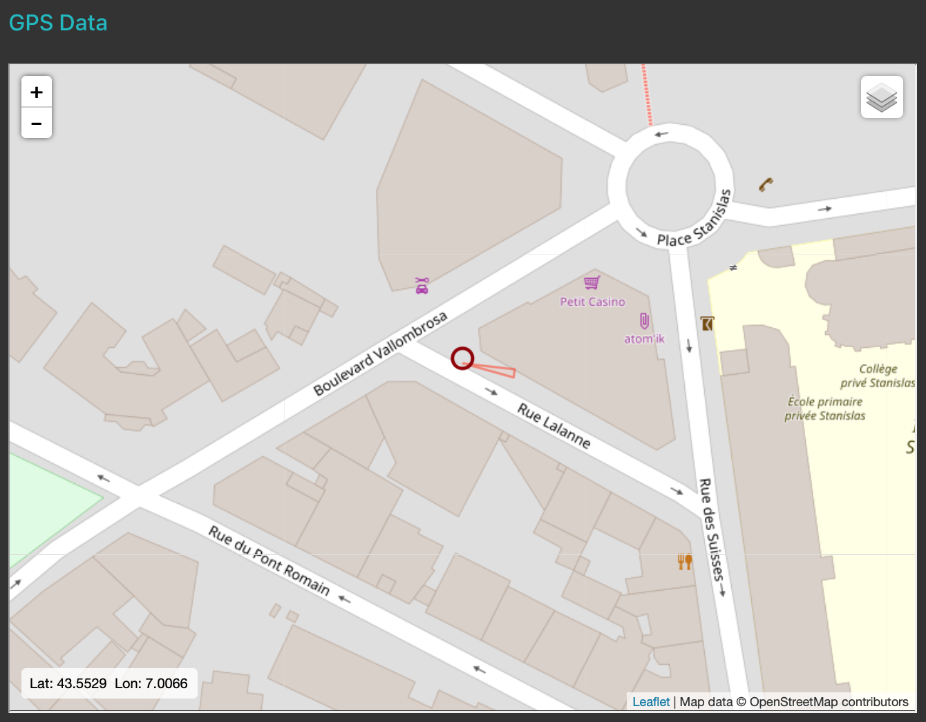 Figure 2
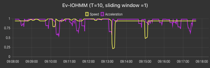 Figure 3
 Figure 4
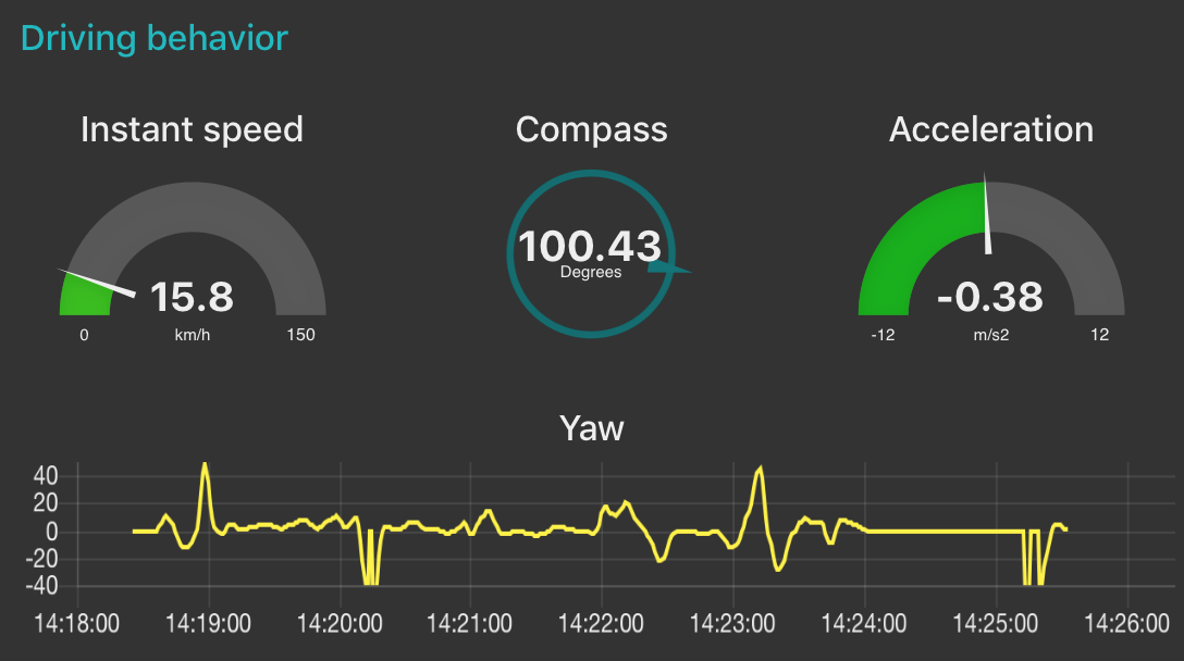 Figure 5
 Figure 6
| Localization | Weather condition | Road | Improved road | Highway | |
| Outside urban area | No precipitation | 90 km/h | 110 km/h | 130 km/h | |
| Rainy | 80 km/h | 100 km/h | 110 km/h | ||
| Visibility <50m | 50 km/h | 50 km/h | 50 km/h | ||
| Urban area | 30 km/h area | 30 km/h | 30 km/h | N/A | |
| General case | 50 km/h | 50 km/h |
|
||
| Improved section | 70 km/h | 70 km/h | N/A |
| OSM Road infrastructure max speed features | Weather data | |||
| From values | maxspeed:<value> | value | hour.precip | mm |
| From localization | zone:maxspeed:FR:30 | 30 km/h | hour.vis | km |
| maxspeed:type:FR:urban | 50 km/h | |||
| maxspeed:type:FR:rural | 90 km/h | |||
| maxspeed:type:FR:trunk | 110 km/h | |||
| maxspeed:type:FR:motorway | 130 km/h | |||
| highway:living_street | 50 km/h | |||
| highway:residential | 50 km/h | |||
| highway:primary | 90 km/h | |||
| highway:secondary | 70 km/h | |||
| highway:tertiary | 50 km/h | |||
| highway:trunk | 110 km/h | |||
| highway:motorway | 130 km/h | |||
Peer Reviews
No public reviews on file for this paper yet. If you reviewed it on a platform where reviews are public (OpenReview, ICLR, NeurIPS, ICML), you can paste yours below so the community can read it here.
Videos
No videos yet. Explain this paper in a talk, walkthrough, or lecture? Add one.
Taxonomy
MethodsSPEED: Separable Pyramidal Pooling EncodEr-Decoder for Real-Time Monocular Depth Estimation on Low-Resource Settings
Effectiveness Assessment of Cyber-Physical Systems
Gérald Rocher
Jean-Yves Tigli
Stéphane Lavirotte
Nhan Le Thanh
GFI Informatique, Saint-Ouen, France
Université Côte d’Azur (UCA), Sophia Antipolis, France
CNRS, laboratoire I3S, Sophia Antipolis, France
Abstract
By achieving their purposes through interactions with the physical world, Cyber-Physical Systems (CPS) pose new challenges in terms of dependability. Indeed, the evolution of the physical systems they control with transducers can be affected by surrounding physical processes over which they have no control and which may potentially hamper the achievement of their purposes. While it is illusory to hope for a comprehensive model of the physical environment at design time to anticipate and remove faults that may occur once these systems are deployed, it becomes necessary to evaluate their degree of effectiveness in vivo. In this paper, the degree of effectiveness is formally defined and generalized in the context of the measure theory. The measure is developed in the context of the Transferable Belief Model (TBM), an elaboration on the Dempster-Shafer Theory (DST) of evidence so as to handle epistemic and aleatory uncertainties respectively pertaining the users’ expectations and the natural variability of the physical environment. The TBM is used in conjunction with the Input/Output Hidden Markov Modeling framework we denote by Ev-IOHMM to specify the expected evolution of the physical system controlled by the CPS and the tolerances towards uncertainties. The measure of effectiveness is then obtained from the forward algorithm, leveraging the conflict entailed by the successive combinations of the beliefs obtained from observations of the physical system and the beliefs corresponding to its expected evolution. The proposed approach is applied to autonomous vehicles and shows how the degree of effectiveness can be used for bench-marking their controller relative to the highway code speed limitations and passengers’ well-being constraints, both modeled through an Ev-IOHMM.
keywords:
Cyber Physical Systems, Degree of Effectiveness, Transferable Belief Model, Input/Output Hidden Markov Model, Zone of Viability
††journal: International Journal of Approximate Reasoning
1 Introduction
Generally, computing systems are understood as being purposeful processing units, directed to produce expected results by means of computational resources manipulating data through controlled computational environments.
At the infrastructure level, some hardware and software mechanisms ensure correct operation of the computing resources (e.g. power-on self-test, etc.), integrity and persistence of the data (e.g. Cyclic Redundancy Check (CRC), memory content refresh, etc.). At the system level, accesses to the computational resources are made safe by an operating system or a middleware. The computational environments being controlled, the production and the persistence of the expected results are guaranteed ”by design” solely provided that the computer program issues the right commands to the computational resources. In this sense, a computer program is a perfect deterministic model of a computing system and the question does not even arise that, x being a variable, the execution of the following code snippet will lead its value to be set to 6 into the memory.
Let us now consider Cyber-Physical Systems (CPS) as being orchestrations of distributed computing and physical systems [1]. CPS can be understood as being ”cyber” physical processes where some properties of a physical system of interest are purposefully modified by means of computational resources manipulating them through transducers (e.g. sensors and actuators). For instance, let us keep the template of the preceding code snippet by considering that the variable to be modified now corresponds to a physical property of the physical system (e.g. the temperature in a living room).
What trust can we have that the temperature in the living room is going to be changed to \SI23\degC? In other words, can one consider the above code snippet as a perfect deterministic model of the physical system? Considering that the living room is a non-isolated physical system, the answer is ”no”. Such systems are driven by non-deterministic dynamics, at any time, the temperature of the living room can be affected by surrounding processes over which the computing system has no control [2] [3] [4]. This situation is aggravated for the Internet of Things (IoT)-based CPS whose underlying infrastructure is volatile. Indeed, their structural components being embedded into physical things, their availability cannot be ensured over time. Consequently, the attainment of the CPS purposes cannot be guaranteed solely ”by design” [1].
As a solution to this problem, we propose to quantitatively assess, at run-time, to which extent the CPS purposes are met. In other words, it is about providing the degree of effectiveness of the CPS as a measure of the concrete evolution of the physical system according to the expected evolution. To be more precise about the measure and the meaning we seek to give it as an assessment of the degree of effectiveness of the CPS, we borrow some terminology employed in the viability theory [5]. Let us assume that the expected evolution of the physical system can be specified as a deterministic model, free from uncertainties, where (1) state transitions are determined by contextual events (stimuli), (2) states are qualified by the expected physical effects resulting from actuators over which the computing system has control. Zones of Viability extend this deterministic point of view with tolerances accounting for aleatory uncertainties pertaining the natural variability of actuators effects and sensors readings and for epistemic uncertainties relative to the users’ satisfaction towards the concrete evolution of the physical system.
In this paper, we propose to generalize the deterministic model in the framework of the measure theory. Doing so, one can leverage the set of measures (probabilities, possibilities, etc.) as a means of defining zones of viability from which one can reason in order to obtain the degree of effectiveness. By obtaining a quantitative measure of the degree of effectiveness, (1) one can leverage this measure within a feedback loop so as for the controller of the system to minimize the behavioral drift (e.g. negative feedback control systems [6]), (2) one can use this measure as a bench-marking tool used to compare algorithms deployed for controlling CPS.
2 Related work and contributions
The work presented in this paper is closely related to the dependability of the computing systems [7]. Within computer science, this term refers to the trust that can justifiably be placed in the service delivered by computing systems and covers all their critical quality aspects [8]. In other words, it reflects users’ degree of trust in these systems. Among the attributes of dependability [9], availability (i.e. readiness for correct service), reliability (i.e. continuity of correct service), safety (i.e. absence of consequences on the users and the environment) and integrity (i.e. absence of improper system alterations) characterize the immunity of computing systems towards uncontrolled physical processes and associated uncertainties (i.e. threats that can affect computing systems operation and undermine their dependability [9]).
The assessment of the dependability can be done at design time through analytic metrics using models of the systems and, whenever possible, the known uncertainties (e.g. U-Test [10]). Run-time monitoring involves direct and indirect empirical metrics, respectively measuring the system itself through probes (whenever possible) and its effects within the physical environment through sensors.
While methodologies involved at design time (e.g. Model-based design) and at testing phase (e.g. Model checking, simulation, etc.) are respectively devoted to fault prevention and fault removal, run-time monitoring is devoted to automatic fault and anomaly detection [11]. The most common formulation of the anomaly detection problem is to determine if a given test sequence is anomalous with respect to normal sequences. More formally, given a set of normal sequences and a test sequence , it is about computing an anomaly score for , with respect to . It is assumed that test sequences might be misaligned in time and space w.r.t the normal sequences. We do also consider complex, and collective anomalies. On the one hand, when contextual attributes can be associated with observations (e.g. time, location, etc.), contextual anomalies are corresponding to behaviors that are valid under some conditions but are abnormal in others. For instance, in European countries, normally high temperatures during the summer can be considered as contextual anomalies if they occur during the winter (time-based contextual anomaly). On the other hand, collective anomalies correspond to a collection of consecutive behaviors which are not abnormal by themselves but are abnormal when they occur together as a collection [12]. Approaches that address these anomalies fall into three categories described hereafter.
2.1 Prediction-based approaches
**These approaches consist in modeling legitimate behavior through a parametric model learned from observations and further used for predicting observation at each time . Abnormal behaviors are those whose real observations differ from the predicted ones.
**
In [13], authors use stacked Long Short-Term Memory (LSTM) networks [14] for anomaly/fault detection in time series. A network is trained on non-anomalous data and used as a predictor over a number of time steps. The resulting prediction errors are modeled as a multivariate Gaussian distribution, which is used to assess the likelihood of anomalous behavior. In [15], authors present an unsupervised approach to detect cyber-attacks in Cyber-Physical Systems (CPS). A Recurrent Neural Network (RNN) [16] is used as a time series predictor. The Cumulative Sum method is further used to identify anomalies in a replicate of a water treatment plant.
pros & cons: these models are difficult to train [17] and are generally hardly interpretable, their intrinsic structure and parameters making unclear the mapping between the variables and the observations [18]. For instance, such models, once learned make difficult, if not impossible, the modification of their intrinsic parameters in order to tune a posteriori the tolerances pertaining the epistemic uncertainties. More importantly, learning a comprehensive model of the CPS behavior based on observations is often impracticable with regards to their complexity [1].
2.2 Model drift-based approaches
**These approaches are relative to the anomalous evolution of the model parameters. The basic idea is to build a parametric behavioral test model from test sequences as they arrive and compare it with the normal behavioral model. Dissimilarities between models give the anomaly score.
**
Authors in [19] focus on the quantitative measure of concept drift and introduce the notion of drift magnitude whose value can be quantified through distance functions such as Kullback-Leibler Divergence or Hellinger Distance. Close to the idea of concept drift is the notion of Bayesian Surprise [20]. A surprise quantifies how data affects an observer. It quantifies a mismatch between an expectation and what is actually observed by measuring the difference between posterior and prior beliefs of the observer. In [21] authors propose using Bayesian surprise as a measure of the learning progress of reinforcement learning agents.
pros & cons: being based on the distance between prior and posterior beliefs, the main disadvantage of these approaches concerns the speed of convergence to an accurate test model, highly dependent on the number of observations needed to learn it. Hereby, a short time anomalous behavior might be ”attenuated” or even not detected. These approaches are mainly leveraged in autonomic computing and the models@run-time community [22] where an initial model is updated over time taking into account unanticipated evolutions of the environment. In this context, above a given threshold, the quantitative drift value is used to trigger the update of the model with the newly learned parameters, assuming it represents the correct behavior.
2.3 Likelihood-based approaches
**These approaches consist in modeling legitimate behavior through a parametric model and considering abnormal behaviors as those having low ”likelihood” to have been generated by the model.
**
In this category, Dynamic Bayesian networks (DBN) and derivatives (-order Markov chains) are widely used where tolerances towards uncertainties are generally described through probability density functions (pdf). An extension of the Markovian models, denoted by Hidden Markov Models (HMM), consists in considering the case where states of the model are ”hidden” [23], i.e. not directly observable, or partially hidden [24]. Such models are particularly well suited in the context of this paper where it is assumed that while the expected behavior of a CPS can be described a priori, the prior knowledge of its concrete internals and surrounding environment is unlikely available [1]. In this context, the likelihood of a given observation sequence is inferred from the model of the expected behavior of the system by using the probabilistic forward algorithm. This algorithm computes the likelihood of all the possible sequences of hidden states given the observation sequence . The likelihood of a particular sequence of hidden states given the observation sequence is given by:
[TABLE]
Some works have extended the HMM in the framework of the Transferable Belief Model (TBM) [25], an elaboration on the Dempster-Shafer Theory (DST) of evidence where tolerances towards uncertainties are neither described by probabilities but by belief functions. In [26], the author describes previous works in using HMM with TBM [27],[28] in the context of analyzing time series and denoted as Evidential HMM (EvHMM). Probability-based HMM is built upon the Closed World Assumption (CWA), i.e. probabilities are spread on the states defined in the model with , i.e. and . TBM, on his side, is built upon the Open World Assumption (OWA). It allows to associate a belief value (mass of conflict ) to the empty set, i.e. , meant to quantify the degree of inconsistency of the observations with regards to the model. This is coherent with the meaning we seek to give to the measure of effectiveness. In this context, it is proven in [29] that the plausibility of the observation sequence to have been produced by the model, i.e. the plausibility of the model, is given by obtained from the evidential forward algorithm, likewise the likelihood obtained from the probabilistic forward algorithm.
Close to the concern of CPS behavioral analysis, the case of Evidential HMM with application to dynamical system analysis is described in [30]. However, HMM-based methods do not consider state-transitions probabilities governed by inputs necessary in modeling CPS expected behavior.
A way to cope with this limitation is to use the Input/Output HMM (IOHMM), first introduced in [31]. With this modeling framework, state-transitions probabilities are not hardcoded as it is the case with HMMs. Instead, the probability of a state-transition to occur depends on some input values. In this context, the observation sequence consists in an input sequence and an output sequence . In this context, the likelihood of a particular sequence of hidden states given the sequences and is given by :
[TABLE]
pros & cons: a key advantage here is that these models are interpretable, making clear (1) the mapping between the variables and the observations, (2) the description of the zones of viability through probabilities or belief functions. In this category, HMM-based modeling frameworks and more particularly the IOHMM where state-transitions probabilities depend on some input values, are well suited for representing dynamical systems [32][33]. Moreover, such models assume that the internals and the environment of the systems considered are not necessarily known a priori. This makes sense in the context of CPS that, with regards to their complexity, are unlikely to be comprehensively modeled. At best, one can define their expected behavior through the effects they are supposed to produce in response to some events. By assuming OWA, the Ev-IOHMM would be a good candidate so as to compute the degree of effectiveness of CPS. However, to date, no effort has been put on elaborating on such modeling framework.
2.4 Contributions
In this paper, we do extend previous works on the probabilistic and the possibilistic IOHMM likelihood-based approaches respectively described in [34] and [35] in the framework of the TBM (we denote Ev-IOHMM). The work done in [36],[37] and [38] being considered as the starting points, the main contributions of this paper are the following:
The degree of effectiveness is formally defined and generalized in the context of the measure and the viability theories, 2. 2.
The probabilistic IOHMM described in [31] is extended into the TBM framework, resulting in the Ev-IOHMM. To this end, we do rely on previous contributions done on extending HMM to EvHMM [29][27]. The associated evidential forward algorithm is provided and used for inferring the likelihood of the input/output observations to have been generated by the model whose zones of viability are neither defined through probabilities [34] nor possibilities [35] but by belief functions. 3. 3.
The Evaluation of the approach is carried out on a simple yet revealing example, complemented with a list of use-cases emphasizing its interest. Among these use-cases, we do elaborate on a use-case in the domain of autonomous vehicles. The idea is to leverage the proposed approach as means for designers to benchmark the control systems of these vehicles by relying on the measure of their effectiveness against constraints of the highway code relative to speed limitations and passengers well-being, both modeled through an Ev-IOHMM.
3 Mathematical background
3.1 Deterministic model of the expected behavior
In this paper, we do consider physical systems whose expected evolution under a CPS control can be constrained through a deterministic model whose state transitions are determined by contextual events (stimuli) while states are qualified by the expected physical effects resulting from actuators over which the computing system has control. This model is formally defined by:
[TABLE]
with:
- –
,
- –
is the known initial state,
- –
is the finite set of states,
- –
, , is a state-transition function mapping a state and an input vector to a next state . Each element of qualifies the observation of an event supposed to act on the state to yield . In this context, (denoted in the sequel) represents the set of input vectors whose values are supposed to trigger a state-transition from the state to the state .
- –
, is a set-valued output function mapping each state to a set of expected observations while being in state . The elements of , , , qualifies an expected physical effect while being in state .
- –
is a function mapping a state-transition to the set of inputs needed to qualify this state-transition,
- –
is a function mapping a state to the set of outputs needed to qualify this state.
For instance, Fig.1 depicts the expected behavior of a simple CPS whose purpose is to adjust the luminosity (physical property) of a room (the physical system) according to whether an inhabitant is present or not. While no inhabitant is present in the room (characterized by ) then the value provided from the luminosity sensor should be less than 5 (characterized by ). Here .
Here, one may see a parallel with unit tests performed in software engineering for validating an algorithm. Some inputs are provided to the algorithm. The output, resulting from the treatment of these inputs by the algorithm, is compared with an expected output value. In this context, let us imagine one want to test that the sequence leads the sequence of states : the algorithm under test is the one controlling the CPS considered. The deterministic model of the expected behavior, here, plays the role of an unit test defined as follows :
[TABLE]
The result of the test is then computed by :
[TABLE]
without room for tolerance towards uncertainties, the test result can only be PASS or FAIL, i.e. .
However, without being perfect, the luminosity level at 22.8 (state in Fig.1) when an inhabitant is present may be still acceptable and effectiveness . So, one needs to extend the deterministic model allowing to define tolerances pertaining the following uncertainties:
- –
The aleatory uncertainties which are most likely objective and relative to the natural variability of the physical properties of interest whose values over time are most likely distributed around an average value,
- –
The epistemic uncertainties which are most likely subjective and relative to users’ satisfaction towards the physical system evolution.
Besides these uncertainties, one may also consider reliability uncertainties such as:
- –
The spatial uncertainties relative to the sensors location with respect to the physical property of interest,
- –
The hardware uncertainties relative to the sensors accuracy and resolution,
- –
The model uncertainties relative to the designer of the model and its expertise on the application domain.
3.2 Towards its formalization into the measure theory
So as to handle the uncertainties previously described, we propose to generalize the deterministic model in the framework of the measure theory. Doing so, one can leverage the set of measures (probabilities, possibilities, beliefs, etc.) as a means of defining zones of viability from which one can reason in order to obtain the degree of effectiveness.
3.2.1 Background
Before formally generalizing the deterministic model in the framework of the measure theory and defining the degree of effectiveness, let us first review some key concepts of the measure theory. The reader is referred to the literature for details on this theory [39].
Definition 1**.**
(Measure) Let be a measurable space where is a countable set and is a -algebra over . A function is **[40]**:
Monotone if implies , 2. 2.
Normalized if , 3. 3.
Non-negative if , , 4. 4.
Additive if where then ,
The function is said to be an additive measure if it is monotone, non-negative, additive and . It is said to be a non-additive measure if it is monotone, non-negative, non-additive and . A measure is said to be a sub-measure if , .
Definition 2**.**
(Measurable Function) Let and be measurable spaces where and are countable sets and where and are finite -algebras. A function is said measurable if .
For instance, let , and . Let , and . The function , defined by , , and , is measurable. Indeed, , , , , etc.
Definition 3**.**
(Kernel) Let and be measurable spaces where and are countable sets and where and are finite -algebras. A finite kernel from to is a function that satisfies:
- –
* is a measure on ,*
- –
* is measurable.*
and being countable sets, the kernel can be specified as a matrix . One can think of as providing the conditional measure of given . The kernel is referred to as a stochastic kernel (a.k.a. Markov kernel or probability kernel) when and , i.e. .
Definition 4**.**
(Kernel Product) Let , and be measurable spaces. Let and .
Then, one can define the kernel product as a function of and [41] where is a product operator111In the literature, this operator is also known as fusion operator [42].
Theorem 5**.**
(Ionescu-Tulcea Extension Theorem) **[43]** Let us consider a sequence of measurable spaces . Let assume that for each , there exists a kernel from to . Then, for every sequence taking values in there exists a unique measure .
With these key concepts defined, one can generalize the deterministic model described by Eq.3 in the measure theory framework.
3.2.2 Generalizing the function to the finite kernel
Let us consider the measurable spaces and where is the finite set of states, is the input vector, is a finite -algebra on and is a finite -algebra on . A finite kernel from to is defined by (Definition.3):
[TABLE]
being a countable set, the kernel can be specified as a matrix . Think of as the conditional measure that the process will be in the state at time given its state at time is and the input vector is . Here, it is assumed that the state at time depends on the state at time and not on the previous states (first order Markov property). Thus, , where and are random variables taking values in and respectively, is a chain with kernels and initial distribution where is a measure on at .
3.2.3 Generalizing the function to the finite kernel
Let us consider the measurable spaces and where is the output vector and is a -algeba on . A finite kernel from to is defined by:
[TABLE]
Think of as the conditional measure that the process is in the state at time given the output vector at time .
Per Definition.4, at each time , the Markov transition kernel , is a function of and (Fig.2). Think of as the conditional measure of given , and .
3.3 Transferable Belief Model (TBM)
3.3.1 Basic definitions and notations
Let us consider the discrete frame of discernment (FoD) representing the states of a physical system where are hypothesis. In this paper, hypothesis are supposed to be exhaustive and exclusive, i.e. the system cannot be in two states at once. A mass function , a.k.a. Basic Belief Assignment (BBA) is defined by:
[TABLE]
where . A BBA is non-additive, i.e
[TABLE]
This is a fundamental difference with probability theory. A proposition explicitly represents the doubt between hypothesis composing and the mass of belief assigned to is not informative regarding the elements of .
A BBA is a set of belief masses concerning propositions verifying:
[TABLE]
is a focal element of the BBA if .
In the Dempster-Shafer theory of evidence is constrained to 0. This constraint is relaxed in TBM [25] where is given different interpretations [44]:
Inaccuracy of the sensors measurements (Observations),
Incompleteness of the model leading to non-exhaustive FoD.
3.3.2 Belief functions
BBAs can be transformed to one-to-one relationships [25] representing the same information (a.k.a. belief functions), albeit in different forms. Some are described hereafter.
- –
Plausibility where
[TABLE]
and reversely
[TABLE]
- –
Belief where
[TABLE]
- –
Commonality where
[TABLE]
and reversely
[TABLE]
3.3.3 CRC/DRC combination rules
There have been many combination rules proposed in the literature [45]. In the sequel, we do consider the Conjunctive Rule of Combination (CRC) and the Disjunctive Rule of Combination (DRC).
Definition 6**.**
**Conjunctive Rule of Combination (CRC). Let us consider two BBAs defined by and .
Assuming their sources are independent and reliable then the unnormalized conjunctive rule of combination (CRC \operatorname*{\scalerel*{\leavevmode\hbox to14.7pt{\vbox to14.7pt{\pgfpicture\makeatletter\hbox{\hskip 7.34819pt\lower-7.34819pt\hbox to0.0pt{\pgfsys@beginscope\pgfsys@invoke{ }\definecolor{pgfstrokecolor}{rgb}{0,0,0}\pgfsys@color@rgb@stroke{0}{0}{0}\pgfsys@invoke{ }\pgfsys@color@rgb@fill{0}{0}{0}\pgfsys@invoke{ }\pgfsys@setlinewidth{0.4pt}\pgfsys@invoke{ }\nullfont\hbox to0.0pt{\pgfsys@beginscope\pgfsys@invoke{ }{ {{}}\hbox{\hbox{{\pgfsys@beginscope\pgfsys@invoke{ }{{}{{{}}}{{}}{}{}{}{}{}{}{}{}{}{{}\pgfsys@moveto{7.1482pt}{0.0pt}\pgfsys@curveto{7.1482pt}{3.94788pt}{3.94788pt}{7.1482pt}{0.0pt}{7.1482pt}\pgfsys@curveto{-3.94788pt}{7.1482pt}{-7.1482pt}{3.94788pt}{-7.1482pt}{0.0pt}\pgfsys@curveto{-7.1482pt}{-3.94788pt}{-3.94788pt}{-7.1482pt}{0.0pt}{-7.1482pt}\pgfsys@curveto{3.94788pt}{-7.1482pt}{7.1482pt}{-3.94788pt}{7.1482pt}{0.0pt}\pgfsys@closepath\pgfsys@moveto{0.0pt}{0.0pt}\pgfsys@stroke\pgfsys@invoke{ } }{{{{}}\pgfsys@beginscope\pgfsys@invoke{ }\pgfsys@transformcm{1.0}{0.0}{0.0}{1.0}{-3.33334pt}{-2.77779pt}\pgfsys@invoke{ }\hbox{{\definecolor{pgfstrokecolor}{rgb}{0,0,0}\pgfsys@color@rgb@stroke{0}{0}{0}\pgfsys@invoke{ }\pgfsys@color@rgb@fill{0}{0}{0}\pgfsys@invoke{ }\hbox{{\cap}} }}\pgfsys@invoke{\lxSVG@closescope }\pgfsys@endscope}}} \pgfsys@invoke{\lxSVG@closescope }\pgfsys@endscope}}} } \pgfsys@invoke{\lxSVG@closescope }\pgfsys@endscope{{{}}}{}{}\hss}\pgfsys@discardpath\pgfsys@invoke{\lxSVG@closescope }\pgfsys@endscope\hss}}\lxSVG@closescope\endpgfpicture}}}{\textstyle\sum}}) can be used as follows [37]: **
, by:
[TABLE]
[TABLE]
This combination may result in a sub-normal BBA, i.e. . The mass of conflict is given by:
[TABLE]
It is worth noting that the CRC can be computed from commonality functions:
[TABLE]
Definition 7**.**
**Disjunctive Rule of Combination (DRC).
Let us consider two BBAs defined by and .
Assuming their sources are independent and at least one source is reliable, then the unnormalized disjunctive rule of combination (DRC \operatorname*{\scalerel*{\leavevmode\hbox to14.7pt{\vbox to14.7pt{\pgfpicture\makeatletter\hbox{\hskip 7.34819pt\lower-7.34819pt\hbox to0.0pt{\pgfsys@beginscope\pgfsys@invoke{ }\definecolor{pgfstrokecolor}{rgb}{0,0,0}\pgfsys@color@rgb@stroke{0}{0}{0}\pgfsys@invoke{ }\pgfsys@color@rgb@fill{0}{0}{0}\pgfsys@invoke{ }\pgfsys@setlinewidth{0.4pt}\pgfsys@invoke{ }\nullfont\hbox to0.0pt{\pgfsys@beginscope\pgfsys@invoke{ }{ {{}}\hbox{\hbox{{\pgfsys@beginscope\pgfsys@invoke{ }{{}{{{}}}{{}}{}{}{}{}{}{}{}{}{}{{}\pgfsys@moveto{7.1482pt}{0.0pt}\pgfsys@curveto{7.1482pt}{3.94788pt}{3.94788pt}{7.1482pt}{0.0pt}{7.1482pt}\pgfsys@curveto{-3.94788pt}{7.1482pt}{-7.1482pt}{3.94788pt}{-7.1482pt}{0.0pt}\pgfsys@curveto{-7.1482pt}{-3.94788pt}{-3.94788pt}{-7.1482pt}{0.0pt}{-7.1482pt}\pgfsys@curveto{3.94788pt}{-7.1482pt}{7.1482pt}{-3.94788pt}{7.1482pt}{0.0pt}\pgfsys@closepath\pgfsys@moveto{0.0pt}{0.0pt}\pgfsys@stroke\pgfsys@invoke{ } }{{{{}}\pgfsys@beginscope\pgfsys@invoke{ }\pgfsys@transformcm{1.0}{0.0}{0.0}{1.0}{-3.33334pt}{-2.77779pt}\pgfsys@invoke{ }\hbox{{\definecolor{pgfstrokecolor}{rgb}{0,0,0}\pgfsys@color@rgb@stroke{0}{0}{0}\pgfsys@invoke{ }\pgfsys@color@rgb@fill{0}{0}{0}\pgfsys@invoke{ }\hbox{{\cup}} }}\pgfsys@invoke{\lxSVG@closescope }\pgfsys@endscope}}} \pgfsys@invoke{\lxSVG@closescope }\pgfsys@endscope}}} } \pgfsys@invoke{\lxSVG@closescope }\pgfsys@endscope{{{}}}{}{}\hss}\pgfsys@discardpath\pgfsys@invoke{\lxSVG@closescope }\pgfsys@endscope\hss}}\lxSVG@closescope\endpgfpicture}}}{\textstyle\sum}}) can be used as follows [37]: **
[TABLE]
[TABLE]
4 Degree of effectiveness
4.1 Formalization in the measure theory
On the basis of the formalization of the deterministic model of the CPS expected behavior in the measure theory described in 3.2 and extending Eq.4, the degree of effectiveness can be formulated as follows:
Definition 8**.**
The degree of effectiveness is a function such that given the state sequence and the observation sequence , the degree of effectiveness is given by:
[TABLE]
The process consists in propagating the measure over the state sequence . At each time , it satisfies a ”prediction () - update ()” mechanism. It can be understood as the ’likelihood’ of the state sequence to have been produced by the observation sequence . gives the measure of the state sequence to start by the state .
As Eq.21 provides the degree of effectiveness for one possible sequence of states, one needs to find the sequence of states leading the highest degree of effectiveness over all the possible sequences of states given the observation sequence, i.e.
[TABLE]
Note 1**.**
The chain where ,* and are random variables taking values in , and respectively, with transition kernel and initial distribution , is an Input/Output Hidden Markov Model (IOHMM)222In this paper we do assume that the state at time only depends on the state at time and not on the previous states (first order Markov chain). [46] (claim derived from [47]).*
Following this definition, an observation sequence is said perfect when
[TABLE]
To be more precise about the meaning we seek to give to the degree of effectiveness, we borrow some terminology employed in the viability theory [5]. Let us consider that the constraints the physical system evolution has to comply with are encoded into information . Then, the following definitions are adopted:
Definition 9**.**
A zone of comfort associated to an event at time corresponds to the set of values for which the event is certain according to I, such that:
[TABLE]
Definition 10**.**
A zone of tolerance associated to an event at time corresponds to the set of values for which the event is uncertain according to I, such that:
[TABLE]
Definition 11**.**
A zone of viability associated to an event at time corresponds to the union of and . Note that outside the zone of viability, the event is impossible according to I:
[TABLE]
Thus, the degree of effectiveness determines zones of viability according to the model, i.e. it determines the boundaries of the states defined in the model. When , one faces a model breakdown, i.e. the state of the system is outside the boundaries of the states defined in the model.
The Fig.3 provides an illustrative example. Here, the event E can be stated as ”the passengers of the ship are safe”. An input of the model might be the geographic position of the ship (latitude/longitude), while the output might be the heart rate of the passengers. Within the zone of comfort one can be certain that the passengers are safe, i.e. their heart rate is at the expected level. Within the zone of tolerance, passengers may suffer from disturbances and their safety is at risk, i.e. their heart rate is higher than expected. The ship is not supposed to go outside the boundary of the zone of viability…
4.2 Application to the Transferable Belief Model
Per Eq.21 and Eq.22, by replacing kernels and with BBAs, the computation of the degree of effectiveness can be factored as follows :
[TABLE]
where represents a belief function defined on conditionally to the subset . For the sake of simplicity, is replaced by in the sequel. It is worth noting that in Eq.26 the masses involved in the computation are supposed to be known.
4.3 Evidential Input/Output Hidden Markov Model (Ev-IOHMM)
The work presented in this paper extends works done on Evidential HMM (Ev-HMM) [26][27] and probabilistic Input/Output HMM (IOHMM) [31]. In the sequel, we do assume the reader is familiar with basics in HMM.
Formally, an Evidential IOHMM (Ev-IOHMM) is defined by the tuple where:
- –
is the finite set of hidden states, i.e. the frame of discernment,
- –
is the emission vector whose elements represent the beliefs conditional to the output value . For instance, represents the belief in at time given the output observation at time t.
- –
is the state-transition matrix. There is one row per singleton . Each row of the matrix is a BBA whose elements represent the belief in transiting from the singleton to this element. For instance, in Ev-HMM, represents the belief in transitioning to state at time given the state at time was . Here the belief is only conditional to the previous state. In Ev-IOHMM, the belief in transitioning from one state to another is also conditional to an input. For instance, represents the belief in transitioning to state at time given the state at time was and the input value was ..
- –
is a vacuous BBA, i.e. meant to indicate that one has no information on the initial state of the system.
Note 2**.**
In real life applications, BBAs are often not directly available. Only the probability or the possibility values computed from observations are available on the singletons. So, the model is extended with a vector and a matrix whose elements describe probability density functions or distributions of possibility :
- –
* is a vector where each element , is a probability density function or distribution of possibility. For instance, denotes the probability of observing the output vector at time given the state is at time .*
- –
* is a matrix where each element , is a probability density function or distribution of possibility. For instance, denotes the probability of transiting to at time , given the state is at time and the input vector is at time .*
The distributions in and can be defined by the designer of the model when distributions represent, for instance, users’ preferences or specific behavioral requirements/constraints. However, to date, no effort has been put on learning the model parameters from observations (following what has been done in **[26]** on the Ev-HMM or in **[49]** for the IO-HMM).
The HMM modeling framework and derivatives rely on computationally efficient reasoning algorithms [50]. Among these algorithms, the forward algorithm offers a solution to the evaluation problem. It computes the ”likelihood” of the observation sequences and to have been produced by the model by taking into account all the possible underlying state sequences. In other words, it provides a solution to the equation Eq.26.
4.3.1 State prediction
Given this model, let us now detail the basic mechanics of the Ev-IOHMM state-prediction. Let us consider the two states model depicted in Fig.4 extending the model depicted in Fig.1 with constraints taking into account uncertainties described as distributions of possibility as depicted in Fig.5.
Let us assume that the input at time was 3.5. Recall that constraints are encoded in the form of probability or possibility functions. So, one needs to compute the possibility value of the input value for each state-transition in the matrix . It gives:
[TABLE]
Now, beliefs allocated to the subsets , i.e. elements of the matrix A, can be deduced from beliefs on the singletons obtained from the observations and the distributions of possibility described in matrix A’ as follows.
- –
When beliefs on singletons are obtained from probability density functions (likelihoods ), one can obtain commonality by [51]:
[TABLE]
- –
When beliefs on singletons are obtained from possibility distributions , one can obtain plausibility by [52]:
[TABLE]
By applying Eq.29 and then Eq.11 for transforming to , one obtains:
[TABLE]
[TABLE]
For the time being, only the BBAs conditional to the singletons and are available. So, one needs to compute beliefs conditional to the subsets and . Per [37], this can be achieved by applying a DRC on BBAs conditional to the singletons as follows:
[TABLE]
For instance, m^{\Omega_{(t)}}_{a}[\Omega]=m^{\Omega_{(t)}}_{a}[x_{1_{(t-1)}}]\operatorname*{\scalerel*{\leavevmode\hbox to14.7pt{\vbox to14.7pt{\pgfpicture\makeatletter\hbox{\hskip 7.34819pt\lower-7.34819pt\hbox to0.0pt{\pgfsys@beginscope\pgfsys@invoke{ }\definecolor{pgfstrokecolor}{rgb}{0,0,0}\pgfsys@color@rgb@stroke{0}{0}{0}\pgfsys@invoke{ }\pgfsys@color@rgb@fill{0}{0}{0}\pgfsys@invoke{ }\pgfsys@setlinewidth{0.4pt}\pgfsys@invoke{ }\nullfont\hbox to0.0pt{\pgfsys@beginscope\pgfsys@invoke{ }{ {{}}\hbox{\hbox{{\pgfsys@beginscope\pgfsys@invoke{ }{{}{{{}}}{{}}{}{}{}{}{}{}{}{}{}{{}\pgfsys@moveto{7.1482pt}{0.0pt}\pgfsys@curveto{7.1482pt}{3.94788pt}{3.94788pt}{7.1482pt}{0.0pt}{7.1482pt}\pgfsys@curveto{-3.94788pt}{7.1482pt}{-7.1482pt}{3.94788pt}{-7.1482pt}{0.0pt}\pgfsys@curveto{-7.1482pt}{-3.94788pt}{-3.94788pt}{-7.1482pt}{0.0pt}{-7.1482pt}\pgfsys@curveto{3.94788pt}{-7.1482pt}{7.1482pt}{-3.94788pt}{7.1482pt}{0.0pt}\pgfsys@closepath\pgfsys@moveto{0.0pt}{0.0pt}\pgfsys@stroke\pgfsys@invoke{ } }{{{{}}\pgfsys@beginscope\pgfsys@invoke{ }\pgfsys@transformcm{1.0}{0.0}{0.0}{1.0}{-3.33334pt}{-2.77779pt}\pgfsys@invoke{ }\hbox{{\definecolor{pgfstrokecolor}{rgb}{0,0,0}\pgfsys@color@rgb@stroke{0}{0}{0}\pgfsys@invoke{ }\pgfsys@color@rgb@fill{0}{0}{0}\pgfsys@invoke{ }\hbox{{\cup}} }}\pgfsys@invoke{\lxSVG@closescope }\pgfsys@endscope}}} \pgfsys@invoke{\lxSVG@closescope }\pgfsys@endscope}}} } \pgfsys@invoke{\lxSVG@closescope }\pgfsys@endscope{{{}}}{}{}\hss}\pgfsys@discardpath\pgfsys@invoke{\lxSVG@closescope }\pgfsys@endscope\hss}}\lxSVG@closescope\endpgfpicture}}}{\textstyle\sum}}m^{\Omega_{(t)}}_{a}[x_{2_{(t-1)}}]. Results are given in Table.4.
[TABLE]
We are now ready to compute states prediction at time given states at time . The prediction is obtained using the following generalized conjunctive form [37]:
[TABLE]
where corresponds to the matrix given in Table.4. Without an a priori on the previous states, i.e. , the predicted BBA is given from Eq.31 further transformed to :
[TABLE]
4.3.2 State emission
Let us also assume that the output at time is 2.34. So, one needs to compute the possibility value of the output value for each state from the vector from which the BBA can further be computed. It gives:
[TABLE]
By applying Eq.29 and then Eq.11 for transforming to , one obtains:
[TABLE]
[TABLE]
In the sequel, the Ev-IOHMM forward algorithm is detailed. This algorithm computes the likelihood of the observation sequences in the form of a BBA from which the degree of effectiveness is computed.
Note 3**.**
The forward algorithm described in the next section makes use of the CRC (7) for propagating beliefs. Other combination rules such as the Cautious Conjunctive Rule of Combination (CCRC) and the Bold Disjunctive Rule of Combination (BDRC) have been introduced in the TBM framework [53]. However, it is shown that the CRC is the only rule satisfying the Shafer-Shenoy axioms for belief functions propagation [54][55].
{comment}
4.3.3 The Ev-IOHMM Forward algorithm
The Ev-IOHMM forward algorithm is close to the Ev-HMM forward algorithm described in [26] and [30]. The main difference consists in conditioning the state-transition not only on the previous state but also on the input observation . Thus, the forward algorithm is given by :
**Initialization
**no a priori is given to the initial state of the system, i.e. . Thus,
[TABLE]
**Induction
**,
[TABLE]
It is worth noting that, at each time , the resulting has to be transformed to by using Eq.14. Thus, one obtain the BBA resulting from the combination of the belief at time with the previous beliefs combined together. However, successive combinations lead the conflict to increase over time, i.e.
[TABLE]
So as to cope with this problem, the BBA is normalized at each time (from ) by redistributing the conflict over propositions . Several strategies have been defined for redistributing the conflict [56] so as to keep at each time . For instance, assuming sources are equally reliable and {m_{1\operatorname*{\scalerel*{\leavevmode\hbox to12.08pt{\vbox to12.08pt{\pgfpicture\makeatletter\hbox{\hskip 6.03838pt\lower-6.03838pt\hbox to0.0pt{\pgfsys@beginscope\pgfsys@invoke{ }\definecolor{pgfstrokecolor}{rgb}{0,0,0}\pgfsys@color@rgb@stroke{0}{0}{0}\pgfsys@invoke{ }\pgfsys@color@rgb@fill{0}{0}{0}\pgfsys@invoke{ }\pgfsys@setlinewidth{0.4pt}\pgfsys@invoke{ }\nullfont\hbox to0.0pt{\pgfsys@beginscope\pgfsys@invoke{ }{ {{}}\hbox{\hbox{{\pgfsys@beginscope\pgfsys@invoke{ }{{}{{{}}}{{}}{}{}{}{}{}{}{}{}{}{{}\pgfsys@moveto{5.83838pt}{0.0pt}\pgfsys@curveto{5.83838pt}{3.22449pt}{3.22449pt}{5.83838pt}{0.0pt}{5.83838pt}\pgfsys@curveto{-3.22449pt}{5.83838pt}{-5.83838pt}{3.22449pt}{-5.83838pt}{0.0pt}\pgfsys@curveto{-5.83838pt}{-3.22449pt}{-3.22449pt}{-5.83838pt}{0.0pt}{-5.83838pt}\pgfsys@curveto{3.22449pt}{-5.83838pt}{5.83838pt}{-3.22449pt}{5.83838pt}{0.0pt}\pgfsys@closepath\pgfsys@moveto{0.0pt}{0.0pt}\pgfsys@stroke\pgfsys@invoke{ } }{{{{}}\pgfsys@beginscope\pgfsys@invoke{ }\pgfsys@transformcm{1.0}{0.0}{0.0}{1.0}{-2.33333pt}{-1.94444pt}\pgfsys@invoke{ }\hbox{{\definecolor{pgfstrokecolor}{rgb}{0,0,0}\pgfsys@color@rgb@stroke{0}{0}{0}\pgfsys@invoke{ }\pgfsys@color@rgb@fill{0}{0}{0}\pgfsys@invoke{ }\hbox{{\cap}} }}\pgfsys@invoke{\lxSVG@closescope }\pgfsys@endscope}}} \pgfsys@invoke{\lxSVG@closescope }\pgfsys@endscope}}} } \pgfsys@invoke{\lxSVG@closescope }\pgfsys@endscope{{{}}}{}{}\hss}\pgfsys@discardpath\pgfsys@invoke{\lxSVG@closescope }\pgfsys@endscope\hss}}\lxSVG@closescope\endpgfpicture}}}{\textstyle\sum}}2}^{\Omega}}(\emptyset)<1, the Dempster’s normalization rule redistributes conflict on the focal elements, i.e. and {m_{1\operatorname*{\scalerel*{\leavevmode\hbox to12.08pt{\vbox to12.08pt{\pgfpicture\makeatletter\hbox{\hskip 6.03838pt\lower-6.03838pt\hbox to0.0pt{\pgfsys@beginscope\pgfsys@invoke{ }\definecolor{pgfstrokecolor}{rgb}{0,0,0}\pgfsys@color@rgb@stroke{0}{0}{0}\pgfsys@invoke{ }\pgfsys@color@rgb@fill{0}{0}{0}\pgfsys@invoke{ }\pgfsys@setlinewidth{0.4pt}\pgfsys@invoke{ }\nullfont\hbox to0.0pt{\pgfsys@beginscope\pgfsys@invoke{ }{ {{}}\hbox{\hbox{{\pgfsys@beginscope\pgfsys@invoke{ }{{}{{{}}}{{}}{}{}{}{}{}{}{}{}{}{{}\pgfsys@moveto{5.83838pt}{0.0pt}\pgfsys@curveto{5.83838pt}{3.22449pt}{3.22449pt}{5.83838pt}{0.0pt}{5.83838pt}\pgfsys@curveto{-3.22449pt}{5.83838pt}{-5.83838pt}{3.22449pt}{-5.83838pt}{0.0pt}\pgfsys@curveto{-5.83838pt}{-3.22449pt}{-3.22449pt}{-5.83838pt}{0.0pt}{-5.83838pt}\pgfsys@curveto{3.22449pt}{-5.83838pt}{5.83838pt}{-3.22449pt}{5.83838pt}{0.0pt}\pgfsys@closepath\pgfsys@moveto{0.0pt}{0.0pt}\pgfsys@stroke\pgfsys@invoke{ } }{{{{}}\pgfsys@beginscope\pgfsys@invoke{ }\pgfsys@transformcm{1.0}{0.0}{0.0}{1.0}{-2.33333pt}{-1.94444pt}\pgfsys@invoke{ }\hbox{{\definecolor{pgfstrokecolor}{rgb}{0,0,0}\pgfsys@color@rgb@stroke{0}{0}{0}\pgfsys@invoke{ }\pgfsys@color@rgb@fill{0}{0}{0}\pgfsys@invoke{ }\hbox{{\cap}} }}\pgfsys@invoke{\lxSVG@closescope }\pgfsys@endscope}}} \pgfsys@invoke{\lxSVG@closescope }\pgfsys@endscope}}} } \pgfsys@invoke{\lxSVG@closescope }\pgfsys@endscope{{{}}}{}{}\hss}\pgfsys@discardpath\pgfsys@invoke{\lxSVG@closescope }\pgfsys@endscope\hss}}\lxSVG@closescope\endpgfpicture}}}{\textstyle\sum}}2}^{\Omega}}(A)>0,
[TABLE]
Other normalization rules exist [56]. For instance, Dubois-Prade normalization rule assumes that at least one source is reliable in case of conflict. , the rule is defined by:
[TABLE]
Termination:
In this paper, we do consider leveraging the conflict as a means to provide the degree of effectiveness as done in [26]. Following the proof given in [26] in the context of Ev-HMM where :
[TABLE]
the degree of effectiveness given the Ev-IOHMM and the observation sequence is given by :
[TABLE]
As described in [30], one needs to record the value of the conflict at each time before normalizing the BBA.
Note 4**.**
The degree of effectiveness may also be a good indicator of the quality of the model **[30]**. Indeed, given a perfect sequence of observations, the degree of effectiveness is supposed to be equal to 1.0 (see Definition.9).
5 An application to autonomous vehicles
Autonomous vehicles are gaining momentum in the CPS community. Although promising a breakthrough in terms of traffic optimization and regulation, these vehicles will be unable to fulfil their potential without ensuring safety of passengers and surroundings. Besides the physical environment these vehicles operate in and in which unanticipated events may hamper their operation at any time, these vehicles are also prone to cyber attacks, potential communication infrastructure and electronic devices issues [57]. For designers, it is then about handling the behavior of these vehicles from an holistic point of view rather than considering each part of the system separately [58],[59]. Thus, by modeling the expected behavior of the system taken as a whole rather than considering its internals, the proposed approach is coherent with the holistic point of view.
This section aims at providing a possible application of the method developed throughout the paper to the domain of autonomous vehicles. The proposed application consists in providing autonomous vehicles designers with a bench-marking tool used for assessing the effectiveness of the controllers of these vehicles. Without claiming to be exhaustive, the solution can be used in addition to existing approaches for autonomous vehicles security and safety. Two scenarios are then considered. The first one is about considering the speed limitations in force in France. Such limitation rules are complex and depend on several factors depicted in Table.9.
The idea here is to prevent the vehicle going beyond the maximum speed allowed taking into account factors depicted in Table.9. The second scenario consists in considering passengers’ well being. The idea here is to prevent rapid accelerations and decelerations of the vehicle especially when meeting humps, roundabout, ”giveway”, etc.
5.1 Methodology
OpenStreetMap (OSM) is a collaborative map of the world. It is a powerful source of information about all types of infrastructure features such as roads, trails, side-walks, etc. Specifically, given GPS longitude and latitude, one can retrieve from the repository all information about the infrastructure around. Our approach is to use this repository so as to gather infrastructure information from GPS data at each time as the vehicle moves. Besides OSM, we do use a weather web service (api.weatherbit.io) allowing us to retrieve weather information at the date of interest.
Based on these information, we do first describe the Ev-HMM model corresponding to the first scenario. Table.10 provides a summary of the features provided by OSM regarding the speed limitations and the associated speed limit values further used in the model. Besides speed limitations, the weather web service provides us with precipitation values (in mm) and visibility (in km). Speed limitation values and weather information are used as inputs of the Ev-IOHMM model (multivariate). Instant speed of the vehicle is used as output of the Ev-IOHMM model. All the constraints considered, the model contains 11 states. For the sake of visibility, a partial representation of the model is depicted in Fig.7.
The model for the second scenario is built upon the same approach. The inputs of the associated Ev-IOHMM are gathered from some OSM features of interest, i.e, traffic_calming:hump, traffic_calming:choker, highway:stop and highway:give_way, taking value of ”1.0” if the feature is detected around, ”0.0” otherwise. The output of the Ev-IOHMM corresponds to the constraint on the acceleration and deceleration while being in each state. Instant acceleration and deceleration of the vehicle is computed based on the delta of speed and the delta of the distance travelled between two time steps (). The corresponding Ev-HMM model is depicted in Fig.8.
Note 5**.**
In these scenarios, we do assume the behavioral constraints are defined by the designer of the model. For instance, for the first scenario, the maximum speed limits in force are subject to tolerances inherent to radar systems accuracy (generally, in the 5% range) that cannot be retrieved from learning. For the second scenario, tolerances may be adjusted based on users’ feedback or from their preferences.
5.2 Results
To complete the experimentations, a C# library has been developed based on the Matlab functions developed by Philippe Smets [60]. The library has been further extended with combination rules (CRC and DRC [37]) and normalization rules (Dempster [61], Yager [62], and Dubois-Prade [56]). A mobile phone application is further used for recording GPS data from several drivers. The traces recorded are then post-processed in order to add, based on latitude and longitude information, the OSM infrastructure features of interest near the location of the vehicle along with the weather data, based on timestamp. The post processor aims at generating a dataset that can be replayed from a graphical interface built using Node-Red [63] and in which the Ev-IOHMM models are instantiated for evaluation (see Fig.9 and Fig.10). The degree of effectiveness is then assessed using the Ev-IOHMM models described in Fig.7 and Fig.8.
{comment}
Results are provided in Fig.12. It is worth noting that the proposed approach is not predictive, i.e. the degree of effectiveness is computed based on the last observations. The length depends on the sampling rate of the sensors, the Ev-IOHMM model and the physical process whose evolution is observed. By applying a sliding window on the observations, once the window has been filled up with observations, one can get the computation of the degree of effectiveness performed upon each new observation. Results obtained may help designers of autonomous vehicles to benchmark the controllers for different situations.
6 Conclusion and perspectives
Cyber-Physical Systems (CPS) are computing systems whose purposes are achieved from interactions with the physical world by means of transducers (sensors and actuators). These systems pose new challenges in terms of dependability, the evolution of the physical systems they control being affected by unanticipated physical processes over which they have no control and which may potentially hamper the achievement of their purposes. It is now recognized that designers of such systems can no longer lean, at design time, on comprehensive and reliable models for anticipating and removing faults that may arise once these systems are deployed. Instead, they have to be monitored in vivo and quantitatively evaluated for effectiveness throughout their life cycle.
In this paper, we formally defined and generalized the notion of effectiveness in the context of the measure and viability theories. We further detailed the mathematical properties the measure has to comply with in the context of assessing CPS effectiveness. The measure is further developed in the Transferable Belief Model (TBM) framework, an elaboration of the Dempster-Shafer Theory (DST) of evidence. The proposed approach is intended to have several applications in the context of benchmarking and assessment of Quality of Experience (QoE)[64]:
- –
The measure can be used as a benchmarking tool. For instance, let us consider the case of autonomous driving. One might be interested in comparing algorithms used to control autonomous vehicles according to the highway code. As a future work, we do plan to apply the proposed approach to this use-case based on the UAH-DriveSet [65].
- –
Assuming the expected evolution of the physical system being driven by the CPS is specified by the users (e.g. through end-user programming [66]), the degree of effectiveness might give a direct insight on users’ satisfaction, i.e. QoE as an assessment of the human satisfaction when interacting with technology and business entities in a particular context.
The proposed approach may also provide an added value in self-adaptive systems:
- –
In the context of the Internet of Things (IoT), many physical devices now expose services available to ubiquitous computing systems leveraging them for composing the so-called ambient applications (e.g. smart-home, smart-city, etc.). The question then arises for these systems of how to select the relevant services. Current approaches rely on semantic annotations used to formally describe the services [67][68]. While this approach is relevant, (1) semantic annotations are pure models, agnostic to the target operational environment, (2) the behavior of a composed application cannot be inferred solely given the individual behavior of the services it is composed with. Hence, observing the concrete behavior of these systems and providing them with a feedback through the measure of effectiveness would help them selecting more appropriate services over time.
- –
More generally, self-adaptive systems pose new challenges in term of assurance, i.e. the ability to provide evidence that these systems satisfy their behavioral requirements, irrespective of the adaptations over time [69]. One may envision leveraging the assessment proposed in this paper within a feedback loop providing CPS with self-awareness capability allowing them to react towards any deviation.
However, although promising, the proposed approach suffers from limitations :
- –
The approach is not predictive, the measure is computed based on past events. This could be a problem for safety critical CPS for which an immediate response is required,
- –
As such, the Ev-IOHMM cannot manage temporal constraints which are of importance in the CPS context. Following what has been done on Hidden Semi-Markov Models (HSMM)[70], we do plan to develop the Ev-IOHSMM where temporal constraints are used to specify the maximum amount of time allowed to switch from one state to another one or to specify the maximum time one is allowed to stay in a particular state,
- –
The Ev-IOHMM is memory greedy, it implies elements in the state-transition matrix . For instance, for the first scenario described in section 5, the model of the expected behavior contains 11 states leading a 20482048 state-transition matrix. The complexity in time of the forward algorithm described in 4.3.3 is when using commonalities . By using plausibilities , the complexity is [28]. As a recommendation, when is large, it is preferable to avoid matrix calculus and use the binary format as means to encode focal elements [71],
- –
Finally, it is assumed that sensors required for measuring the effectiveness are available. First, it might not be the case and one needs to assess cost/benefits of adding the required sensors. Second, it might be the case but with sensors not as relevant as desired (for instance, a luminosity sensor is made available but not exactly at the desired location). In that case, one can determine some contextual discounting factors [72], but the challenge remains on the determination of the discounting factor values.
7 Acknowledgment
This work has been supported by GFI Informatique, Innovation group, Saint-Ouen, France. The authors wish to thank the reviewers for their valuable suggestions that greatly helped improve the quality of this paper.
The authors are also thankful to Emmanuel Ramasso ([email protected]) for his help in better understanding some specific points of the TBM theory.
The reference list from the paper itself. Each links out to its DOI / PubMed record.
- 1[1] E. A. Lee, The past, present and future of cyber-physical systems: A focus on models, Sensors 15 (3) (2015) 4837–4869.
- 2[2] D. Garlan, Software engineering in an uncertain world, in: Proceedings of the FSE/SDP workshop on Future of software engineering research, ACM, 2010, pp. 125–128.
- 3[3] T. Bures, D. Weyns, C. Berger, S. Biffl, M. Daun, T. Gabor, D. Garlan, I. Gerostathopoulos, C. Julien, F. Krikava, et al., Software engineering for smart cyber-physical systems–towards a research agenda: Report on the first international workshop on software engineering for smart cps, ACM SIGSOFT Software Engineering Notes 40 (6) (2015) 28–32.
- 4[4] M. Zhang, B. Selic, S. Ali, T. Yue, O. Okariz, R. Norgren, Understanding uncertainty in cyber-physical systems: A conceptual model, in: European Conference on Modelling Foundations and Applications, Springer, 2016, pp. 247–264.
- 5[5] J.-P. Aubin, A. Bayen, P. Saint-Pierre, Viability Theory: New Directions, Springer, Cham, Switzerland, 2011.
- 6[6] R. E. Bellman, Adaptive control processes: a guided tour, Vol. 2045, Princeton university press, 2015.
- 7[7] J.-C. Laprie, Dependability: Basic concepts and terminology, in: Dependability: Basic Concepts and Terminology, Springer, Vienna, Austria, 1992, pp. 3–245.
- 8[8] I. Eusgeld, F. Freiling, R. H. Reussner, Dependability Metrics: GI-Dagstuhl Research Seminar, Dagstuhl Castle, Germany, October 5-November 1, 2005, Advanced Lectures, Vol. 4909, Springer, 2008.