Optimizing the accuracy and efficiency of optical turbulence profiling using adaptive optics telemetry for extremely large telescopes
Douglas J Laidlaw, James Osborn, Timothy J Morris, Alastair G Basden,, Olivier Beltramo-Martin, Timothy Butterley, Eric Gendron, Andrew P Reeves,, G\'erard Rousset, Matthew J Townson, Richard W Wilson

TL;DR
This paper presents a method to improve the accuracy and speed of atmospheric turbulence profiling for adaptive optics in large telescopes by using covariance map regions of interest, validated with real and simulated data.
Contribution
It introduces a covariance map ROI technique for turbulence profiling that enhances accuracy and significantly reduces computational time for extremely large telescopes.
Findings
Covariance map ROI improves turbulence profile accuracy.
Reduces fitting time by a factor of 72 for large systems.
Validated with on-sky and simulated data from CANARY.
Abstract
Advanced adaptive optics (AO) instruments on ground-based telescopes require accurate knowledge of the atmospheric turbulence strength as a function of altitude. This information assists point spread function reconstruction, AO temporal control techniques and is required by wide-field AO systems to optimize the reconstruction of an observed wavefront. The variability of the atmosphere makes it important to have a measure of the optical turbulence profile in real time. This measurement can be performed by fitting an analytically generated covariance matrix to the cross-covariance of Shack-Hartmann wavefront sensor (SHWFS) centroids. In this study we explore the benefits of reducing cross-covariance data points to a covariance map region of interest (ROI). A technique for using the covariance map ROI to measure and compensate for SHWFS misalignments is also introduced. We compare the…
Click any figure to enlarge with its caption.
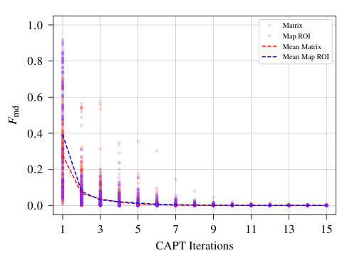 Figure 1
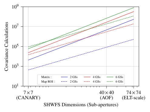 Figure 2
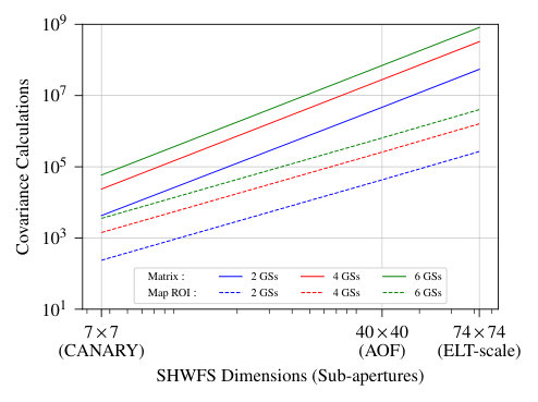 Figure 3
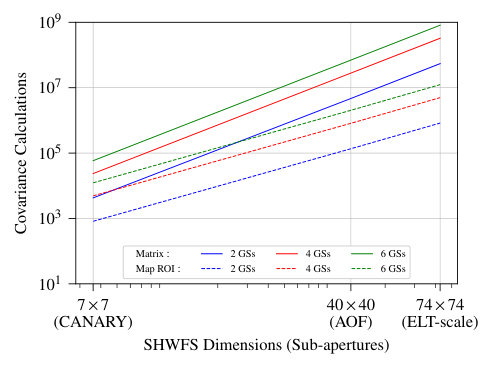 Figure 4
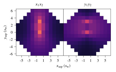 Figure 5
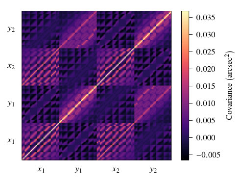 Figure 6
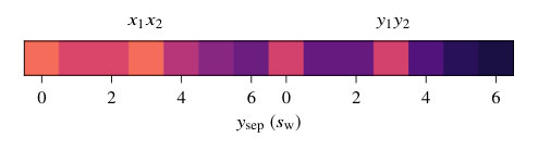 Figure 7
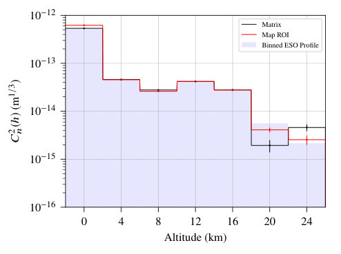 Figure 8
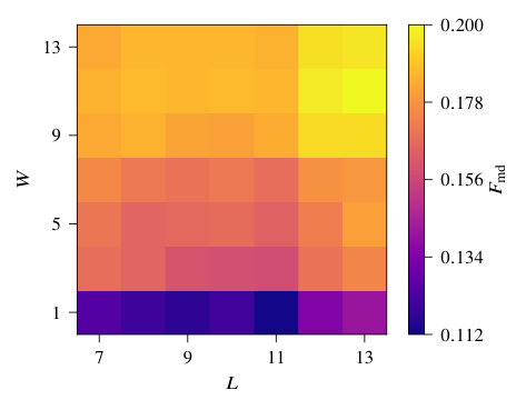 Figure 9
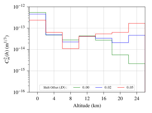 Figure 10
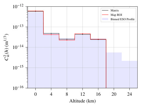 Figure 11
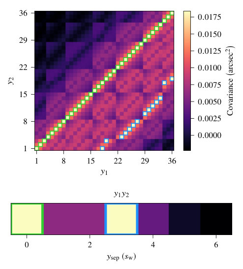 Figure 12
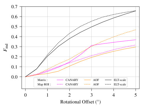 Figure 13
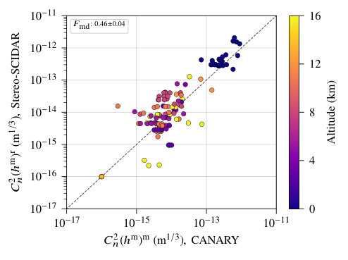 Figure 14
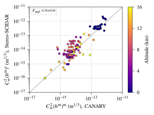 Figure 15
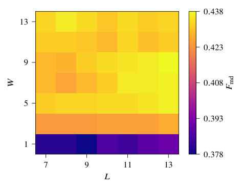 Figure 16
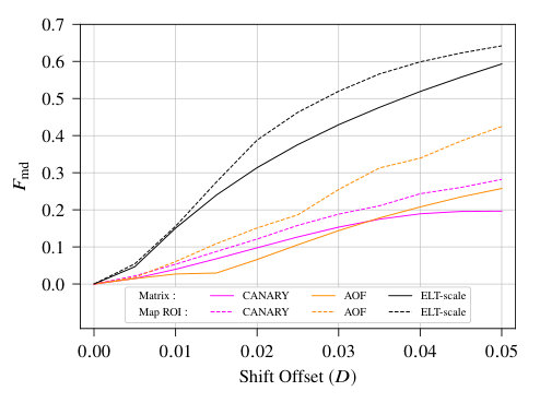 Figure 17
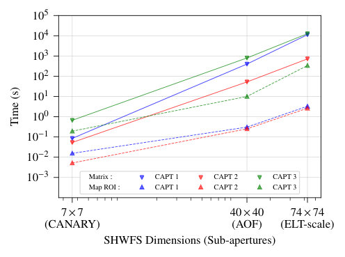 Figure 18
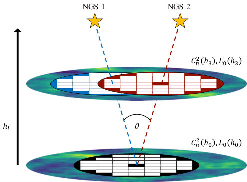 Figure 19
| AO System | Pupil Diameter (m) | SHWFS Dimensions (Sub-apertures) | Sub-apertures per SHWFS | Sub-aperture Baselines per SHWFS |
|---|---|---|---|---|
| CANARY | ||||
| AOF | ||||
| ELT-scale |
| NGS, 024 km | NGS, 016 km | LGS, 016 km | |
| Matrix | 0.19 0.03 | 0.02 0.00 | 0.03 0.00 |
| Map ROI | 0.13 0.03 | 0.03 0.00 | 0.05 0.00 |
| 1 CAPT Iteration | 15 CAPT Iterations | |
| Matrix | 0.46 0.04 | 0.46 0.04 |
| Map ROI | 0.38 0.04 | 0.38 0.04 |
| Matrix | Map ROI | |||||
|---|---|---|---|---|---|---|
| Shift Offset in () | Shift Offset in () | Rotational Offset (∘) | Shift Offset in () | Shift Offset in () | Rotational Offset (∘) | |
| SHWFS.1 | 0.01 | 0.02 | 1.33 | 0.02 | 0.02 | 1.80 |
| SHWFS.2 | 0.02 | 0.00 | 1.14 | 0.03 | 0.01 | 2.11 |
| SHWFS.3 | 0.01 | 0.00 | 1.08 | 0.01 | 0.01 | 1.27 |
| SHWFS.4 | 0.00 | 0.00 | 1.06 | 0.00 | 0.00 | 1.56 |
| Time Taken (s) | ||
|---|---|---|
| Matrix | Map ROI | |
| AO System | CAPT 1+2 | CAPT 1+2 |
| CANARY | 0.09 | 0.02 |
| AOF | 381.14 | 0.04 |
| ELT-scale | 104 | 0.21 |
| Time Taken (s) | ||||
| Matrix | Map ROI | |||
| AO System | CAPT 1+2 | CAPT 3 | CAPT 1+2 | CAPT 3 |
| CANARY | 0.1 | 0.67 | 0.02 | 0.19 |
| AOF | 454.17 | 801.41 | 0.56 | 10.06 |
| ELT-scale | 104 | 104 | 5.93 | 338.52 |
Peer Reviews
No public reviews on file for this paper yet. If you reviewed it on a platform where reviews are public (OpenReview, ICLR, NeurIPS, ICML), you can paste yours below so the community can read it here.
Videos
No videos yet. Explain this paper in a talk, walkthrough, or lecture? Add one.
Optimising the accuracy and efficiency of optical turbulence profiling using adaptive optics telemetry for extremely large telescopes
Douglas J. Laidlaw,1 James Osborn,1 Timothy J. Morris,1 Alastair G. Basden,1 Olivier Beltramo-Martin,2 Timothy Butterley,1 Eric Gendron,3 Andrew P. Reeves,1,4Gérard Rousset,3 Matthew J. Townson,1 and Richard W. Wilson1
1Centre for Advanced Instrumentation (CfAI), Durham University, South Road, Durham, DH1 3LE, United Kingdom.
2Aix Marseille Univ., CNRS, CNES, LAM, 38 rue F. Joliot-Curie, 13388 Marseille Cedex 13, France.
3LESIA, Observatoire de Paris, Universit PSL, CNRS, Sorbonne Universit, Univ. Paris Diderot,
Sorbonne Paris Cit, 5 place Jules Janssen, 92195 Meudon, France.
4Institute of Communication and Navigation, German Aerospace Center (DLR), 82234, Germany E-mail: [email protected]
(Accepted XXX. Received YYY; in original form ZZZ)
Abstract
Advanced adaptive optics (AO) instruments on ground-based telescopes require accurate knowledge of the atmospheric turbulence strength as a function of altitude. This information assists point spread function reconstruction, AO temporal control techniques and is required by wide-field AO systems to optimise the reconstruction of an observed wavefront. The variability of the atmosphere makes it important to have a measure of the optical turbulence profile in real-time. This measurement can be performed by fitting an analytically generated covariance matrix to the cross-covariance of Shack-Hartmann wavefront sensor (SHWFS) centroids. In this study we explore the benefits of reducing cross-covariance data points to a covariance map region of interest (ROI). A technique for using the covariance map ROI to measure and compensate for SHWFS misalignments is also introduced. We compare the accuracy of covariance matrix and map ROI optical turbulence profiling using both simulated and on-sky data from CANARY, an AO demonstrator on the 4.2 m William Herschel telescope, La Palma. On-sky CANARY results are compared to contemporaneous profiles from Stereo-SCIDAR - a dedicated high-resolution optical turbulence profiler. It is shown that the covariance map ROI optimises the accuracy of AO telemetry optical turbulence profiling. In addition, we show that the covariance map ROI reduces the fitting time for an extremely large telescope-scale system by a factor of 72. The software package we developed to collect all of the presented results is now open-source.
keywords:
turbulence - atmospheric effects - instrumentation: adaptive optics - telescopes
††pubyear: 2016††pagerange: Optimising the accuracy and efficiency of optical turbulence profiling using adaptive optics telemetry for extremely large telescopes–Optimising the accuracy and efficiency of optical turbulence profiling using adaptive optics telemetry for extremely large telescopes
1 Introduction
Advanced ground-based optical telescopes can employ adaptive optics (AO) systems to compensate for wavefront perturbations. The primary cause of these aberrations are atmospheric refractive index fluctuations. AO systems are able to detect the strength of phase perturbations across a field of view (FoV) by utilising Shack-Hartmann wavefront sensors (SHWFSs). This information is then relayed to one or more deformable mirrors (DMs) - situated in the optical path - that act to mitigate the measured perturbations. To achieve high angular resolution in wide-field astronomy AO systems must be capable of tomographically reconstructing the wavefront across a large FoV. This technique often requires an estimation of the optical turbulence profile i.e. a measure of the refractive index structure constant, , where is altitude. The optical turbulence profile directly impacts wavefront correction in wide-field AO (Neichel et al., 2009). Precise point spread function (PSF) reconstruction is therefore reliant on the accuracy of its measurement (Villecroze et al., 2012; Martin et al., 2016). Additional applications for optical turbulence profiling include AO temporal control techniques (Petit et al., 2009), queue scheduling of science cases and forecasting of atmospheric parameters (Masciadri & Lascaus, 2012). Forecasts may in turn be validated and calibrated by a subsequent measure of the optical turbulence profile.
Slope Detection and Ranging (SLODAR; Wilson, 2002) is a widely-used technique for measuring the optical turbulence profile. It uses a number of SHWFSs to geometrically triangulate turbulent zones in the atmosphere. SHWFSs are used to measure wavefront perturbations and so the SLODAR technique can utilise AO telemetry. One possible SLODAR-based technique for measuring the optical turbulence profile is to first calculate the cross-covariance between the centroid measurements from all SHWFSs. This expresses the optical turbulence profile as a covariance matrix. The optical turbulence profile can be recovered by iteratively fitting an analytical model to the measured covariance matrix (Vidal et al., 2010). Covariance matrix fitting can also be used for parameter estimation e.g. measuring SHWFS misalignments (Martin et al., 2016). To assure science goals are met forthcoming extremely large telescope (ELT) AO systems must be updated regularly with an accurate measure of the optical turbulence profile (Peng et al., 2018). However, the covariance matrix of an ELT AO system will contain millions of cross-covariance measurements. This makes it a challenge to perform efficient ELT covariance matrix fitting.
By averaging covariance matrix baselines the optical turbulence profile can be studied as a covariance map. Previous studies have shown that a covariance map region of interest (ROI) can be used to perform SLODAR data analysis (Butterley, Wilson & Sarazin, 2006; Cortés et al., 2012; Guesalaga et al., 2014; Guesalaga et al., 2017; Ono et al., 2016). However, an investigation into the optimal size of the covariance map ROI has not been published. We describe our methodology to define the covariance map ROI and we explore its benefits for SLODAR data analysis. It is compared to its covariance matrix counterpart throughout. Three different scales of AO systems are considered: CANARY, a multi-object AO (MOAO) pathfinder on the m William Herschel telescope (WHT), La Palma; the adaptive optics facility (AOF) on an m unit telescope of the very large telescope (VLT), Paranal; and an instrument designed for the m European ELT, Cerro Armazones. The parameters of each AO system are listed in Table 1.
We assess the sensitivity of the two SLODAR methods with respect to SHWFS misalignments in rotation and lateral shift. It was shown by Martin et al. (2016) that the covariance matrix can be used to measure SHWFS misalignments. If these misalignments can be measured they can be compensated for during the optical turbulence profiling procedure. We build upon this work and show that with a modified fitting procedure, the covariance map ROI can also measure SHWFS misalignments.
A qualitative study of AO telemetry optical turbulence profiling compares the accuracy of the two SLODAR methods. The comparison is made using both simulated and on-sky CANARY data (Morris et al., 2014). In additon, we investigate the optimal size of the covariance map ROI. Contemporaneous measurements made using the scintillation detection and ranging (SCIDAR; Vernin et al., 1973) technique were provided as a reference to the expected on-sky optical turbulence profile. These measurements came from the Stereo-SCIDAR instrument (Shepherd et al., 2013) on the 2.5 m Isaac Newton telescope (INT), La Palma (Osborn et al., 2015). The Stereo-SCIDAR instrument does not utilise AO telemetry and instead performs optical turbulence profiling through the cross-covariance of atmospheric scintillation patterns. It is a dedicated stereoscopic high-resolution optical turbulence profiler.
Quantitative analysis is presented for the reduction in computational time when performing SLODAR data analysis with a covariance map ROI instead of a covariance matrix. The potential benefits for an ELT-scale instrument are considered.
2 Measuring the optical turbulence profile
The SLODAR technique has been outlined in previously published literature (for a detailed description see Butterley, Wilson & Sarazin, 2006). We review the key concepts here. The system requires sufficiently bright objects that can be used as Guide Stars (GSs) for wavefront sensing. The optical phase of each GS can then be measured at the ground via independent SHWFSs. Fig. 1 illustrates the sub-aperture optical paths of two optically aligned SHWFSs that are observing independent natural guide stars (NGSs). The distance to NGS sub-aperture optical path intersection in Fig. 1 is given by , where
[TABLE]
In equation 1 is the angular separation between the NGSs. The distance between the centres of two adjacent subapertures is given by . It should be noted that equation 1 is only valid if the NGSs are separated in the FoV of the telescope by a position angle of 0, 90, 180 or . Two altitudes of sub-aperture optical path intersection are shown in Fig. 1. The sub-aperture separation order is denoted . The maximum distance of sub-aperture optical path intersection, ( for the configuration shown in Fig. 1), is therefore , where is the diameter of the telescope. If an ELT-scale instrument and CANARY were observing the same NGS asterism, this implies that would be larger for the ELT-scale instrument by a factor of (see Table 1). The ELT-scale instrument would also have an increased optical turbulence profile altitude-resolution. for CANARY and an ELT-scale instrument would be and , respectively.
It has been shown that the SLODAR method can also utilise laser guide stars (LGSs; Cortés et al., 2012). Due to the cone effect the distance to LGS sub-aperture optical path intersection, , does not scale linearly with . For optically aligned SHWFSs with LGS position angles of 0, 90, 180 or
[TABLE]
where is the distance to the LGSs. Equation 2 assumes that is the same for both LGSs.
The SLODAR technique is able to use SHWFS GS measurements to triangulate atmospheric turbulence strength as a function of altitude (see Section 2.1). These atmospheric aberrations have an outer scale, . Investigations indicate that the outer scale resides between 1-100 m (Ziad et al., 2004). However, using the SLODAR technique the existing class of telescopes do not have the spatial scale to construct an un-biased profile (Ono et al., 2016). It was shown by Guesalaga et al. (2017) that there is no significant difference in SLODAR data analysis when the outer scale is over roughly 3 times the diameter of the telescope pupil. For these reasons it is common practice for the existing class of telescopes to assume m. ELT-scale telescopes might not be able to make this approximation. It is possible that the ELTs will have to measure .
2.1 Covariance matrix
The cross-covariance between all open-loop centroid positions (recorded over some time interval) expresses the optical turbulence profile as a covariance matrix. An analytically generated 2-NGS CANARY covariance matrix is shown in Fig. 2(a). It corresponds the optical turbulence profile illustrated in Fig. 1 i.e. two layers at altitudes of 0 and km. Both turbulent layers are characterised by m and m. is the Fried parameter. Orthogonal measurements from NGS 1 and NGS 2 are given by , and , , respectively. It can be seen in Fig. 2(a) that the lowest signal-to-noise (SNR) cross-covariance measurements are between orthogonal axes. The cross-covariance between sub-apertures from the same SHWFS i.e. the auto-covariance, gives a measure of integrated turbulence strength. The strongest response to the vertical structure of the optical turbulence profile is between equivalent planes of independent SHWFSs e.g. cov and cov.
2.2 Covariance map
We define baseline as the two-dimensional sub-aperture separation between two optically aligned SHWFSs at . The baseline between SHWFSs is characterised by sub-aperture ordering and is therefore independent of any misalignment. The baseline in and is given by and , respectively. The cross-covariance between equivalent planes of independent SHWFSs ( and in Fig. 2(a)) can be averaged as a function of baseline. The resultant array is known as a covariance map. The covariance map from Fig. 2(a) is shown in Fig. 2(b). The covariance map contains all the high SNR information for the vertical structure of the optical turbulence profile. If a system is characterised by random noise then averaging baselines increases the SNR of the optical turbulence profile. Any two GSs in the FoV of the telescope are separated by a position angle, . In Fig. 1 rad and as shown in Fig. 2(b), the optical turbulence profile is primarily projected over sub-aperture separations that are determined by .
2.3 Covariance map region of interest
Measurements within the covariance map can be extracted along the vector projected by - a covariance map Region of Interest (ROI). This requires to be known with respect to the geometry of the SHWFS lenslet array. The covariance map ROI in Fig. 2(c) is taken from the centre of and in Fig. 2(b), and along positive . In reality the optical turbulence profile may not be projected across exact baselines (as it is in Fig. 2(c)). The ROI can compensate for this by encapsulating a larger extent of the map i.e. its length and width can be increased. In this study the length and width of the ROI are denoted by and , respectively. Both and are in units of the distance between two adjacent sub-apertures, . Fig. 2(c) has and , where is the number of SHWFS sub-apertures in one dimension. for the configuration in Fig. 2(c) implies that the ROI includes negative data points e.g. is the same ROI in Fig. 2(c) but with the inclusion of in both and from Fig. 2(b). An ROI of can be thought of as extending the ROI to data points that are projected along . It should be noted that reduces information. There are current as well as forthcoming AO systems that utilise more than two GSs. This assists wide-field AO as it introduces the capability of analysing the optical turbulence profile at multiple altitude resolutions. The covariance map ROI studies the optical turbulence profile in a multi-GS system by stacking the ROI from each GS combination into a single array.
The measured covariance map ROI does not have to come from calculating the covariance matrix and then the covariance map i.e. the steps from Section 2.1 to 2.2. We have developed an algorithm that calculates the covariance map ROI directly from centroid measurements. This process utilises a look-up table that lists sub-aperture combinations as a function of baseline. The algorithm uses with this look-up table to calculate the average cross-covariance at the required baselines.
3 Optical turbulence profiling
It is possible to develop an algorithm for analytically generating the covariance between sub-apertures. Analytical covariance for each turbulent layer depends on , , , sub-aperture separation and optical misregistrations. It should again be noted that baseline is independent of SHWFS misalignments. By analytically generating sub-aperture covariance we are able to iteratively fit an analytical model to SHWFS cross-covariance measurements. This allows us to measure the optical turbulence profile - the idea of the learn stage within learn & apply MOAO tomography (Vidal et al., 2010). For more details on the model fitting procedure and the open-source software package that we have developed see Section 3.2. The reader is directed to Martin et al., 2016 for a complete description of the mathematical procedure that we use for analytically generating sub-aperture covariance.
The approximation we use for analytically generating sub-aperture covariance has been shown to increase in accuracy the further the projected sub-apertures are separated. At sub-aperture separations of zero the analytical model has an overestimation of (Martin et al., 2012). Furthermore, measured covariance at a sub-aperture separation of zero is susceptible to a low SNR. For these reasons the model fitting procedure we use sets the measured cross-covariance between all sub-apertures with baseline to zero. It also sets analytically generated covariance at all baselines to zero.
3.1 Subtracting ground-layer isoplanatic turbulence
The strong ground-layer is usually slow-moving and therefore its cross-covariance function can differ from the analytical model. This makes it difficult to accurately measure the optical turbulence profile at non-zero altitudes. Learn 3 step (L3S; Martin et al., 2016) is a fitting technique used to better detail the optical turbulence profile at non-zero altitudes. It does this by initially subtracting ground-layer isoplanatic turbulence. Subtracting centroid ground-layer isoplanatic turbulence requires calculating the mean centroid location in and for every frame at each sub-aperture baseline. All centroids from every SHWFS then have their respective average at each frame subtracted, removing common-motion at each sub-aperture baseline. In an optically aligned system this common-motion subtraction mitigates ground-layer turbulence. It also simultaneously removes internal vibration artefacts - remnants of wind-shake and telescope tracking errors, seen as a linear addition to cross-covariance measurements with independent values at and . As this treatment is linear the transformation matrix, T, used to perform common-motion subtraction on the SHWFS centroids can be directly applied to an analytically generated covariance matrix. Having A and B represent an analytically generated covariance matrix before and after ground-layer mitigation, respectively, implies that
[TABLE]
An analytical covariance map ROI with subtracted ground-layer isoplanatic turbulence can be calculated by averaging the specific baselines within B (see Section 2.3).
3.2 Covariance parameterisation of optical turbulence and SHWFS misalignments
In this study we use a fitting technique similar to L3S. This decision was based on the fact that L3S has been shown to be robust and to minimise tomographic error (Martin et al., 2012). We use the Levenberg Marquardt algorithm (LMA) to fit an analytical model to SHWFS cross-covariance measurements. The software package we have developed is capable of supervising an AO system by using AO telemetry to measure the optical turbulence profile and SHWFS misalignments in real-time. The user chooses how many layers to fit and the altitudes at which these layers are fitted. Multiple GS combinations can also be fitted to simultaneously. This software package is now open-source111https://github.com/douglas-laidlaw/CAPT (example test cases are included in the open-source package). The software is written in Python and it uses the numpy (van der Walt, Colbert & Gaël, 2011) and scipy (Jones et al., ) libraries. We refer to the AO system supervisor that we have developed as covariance parameterisation of optical turbulence and SHWFS misalignments (CAPT). The three steps of CAPT for a NGS system are as follows.
-
Using the transformation matrix, T, remove centroid common-motion and calculate the chosen cross-covariance array e.g. covariance matrix or map ROI. The LMA fits to measured cross-covariance with an analytically generated covariance array that is ground-layer mitigated. The fit is performed by iteratively adjusting . It is assumed that m.
-
from 1 is used to analytically generate a covariance array that dissociates ground-only turbulence from the complete cross-covariance array (the measured cross-covariance array with no ground-layer mitigation). The LMA fits analytically generated covariance to the measured ground-only cross-covariance array. The fit is performed by iteratively adjusting , and vibration artefacts.
-
Using the parameters recovered from 1 and 2, the LMA fits analytically generated covariance to the complete cross-covariance array by iteratively adjusting SHWFS shift and rotation misalignments.
As mentioned previously the fitting technique we have adopted closely resembles L3S. The differences between CAPT and L3S are listed below.
- •
The first and second steps of L3S remove tip-tilt in both the measured and analytically generated cross-covariance arrays. We found that this did not improve the results and so tip-tilt removal was not included in the first and second steps of CAPT (CAPT 1 and CAPT 2, respectively). Removing tip-tilt also requires an additonal matrix multiplication. Not including this operation therefore improved the efficiency of the system.
- •
The first step of L3S fits and . Although CAPT is capable of fitting an outer scale profile, we do not fit for reasons discussed in Section 2. We fit during CAPT 1 to help account for possible SHWFS misalignments. However, the measurement of is taken from CAPT 2.
- •
The third step of L3S fits vibrational artefacts. We are able to complete this in CAPT 2 as the system is not tip-tilt subtracted. L3S also fits , and vibration artefacts. CAPT does not fit vibrational artefacts as it assumes orthogonal centroids are decorrelated.
- •
The third step of L3S fits SHWFS magnification. We do not fit this parameter during the third step of CAPT (CAPT 3) as this study concentrates on the parameterisation of SHWFS misalignments.
The outer scale measurement in CAPT 2 is not considered physical. It is fitted to acount for the liklihood that the analytical model will differ from the cross-covariance function of the slow-moving ground-layer. During CAPT 1 and CAPT 2, the covariance map ROI has and . In CAPT 3 and . The ROI in CAPT 3 is increased so that it has enough spatial information to detect SHWFS misalignments. These are the dimensions of the covariance map ROI unless stated otherwise. The noise-floor for is set at m1/3 i.e. measurements of m1/3 are made equal to m1/3.
The uplink of LGSs through atmospheric turbulence results in the loss of tip-tilt information. This causes each SHWFS to have an independent tip-tilt term after CAPT 1 ground-layer mitigation. The result of this is a cross-covariance discontinuity within each and measurement. During LGS optical turbulence profiling, CAPT 1 fits linear additions to each and term to account for this discontinuity. In CAPT 2 this fitted parameter is used to help dissociate the ground-layer. It is also included during CAPT 3.
The vertical structure of the optical turbulence profile is dependent on sub-aperture separation. An unknown SHWFS misalignment will therefore directly impact the accuracy of CAPT. SHWFS shift and rotation misalignments are fitted during CAPT 3 however, the optical turbulence profile is recovered during CAPT 1 and CAPT 2. This implies that if an unknown misalignment exists between SHWFSs, the optical turbulence profile will be imprecisely recovered which will lead to CAPT 3 being unable to recover systematic uncertainties. We found that a solution to this problem is to iterate through CAPT several times i.e. run CAPT 1 and CAPT 2, take misalignment measurements from CAPT 3, put them back into CAPT and repeat (see Section 4.2). The idea is that after a number of iterations CAPT will converge on an accurate measure of both and the alignment between the SHWFSs. At the first iteration every layer in the fitted model has a starting point of m and m. Vibrational artefacts and SHWFS misalignments have a starting point of zero. As we iterate through CAPT a number of times, the starting point of each fitted parameter is equal to its measurement from the previous iteration.
4 Results
4.1 SHWFS misalignments and the degradation of optical turbulence profiling
In a physical AO system it is unrealistic to assume perfect optical alignment. It is therefore important to quantify the degradation of covariance matrix and map ROI optical turbulence profiling in the presence of SHWFS misalignments. For CANARY, AOF and ELT-scale configurations, a 2-NGS covariance matrix was analytically generated for 11 evenly-spaced SHWFS rotational misalignments. The maximum offset was . The target covariance matrix (the covariance matrix that would be fitted to), , for each AO system was analytically generated with no noise. This allowed for perfect convergence of centroid cross-covariance measurements to be assumed. Each AO system had generated with such that km and rad. Median atmospheric parameters documented by the European southern observatory (ESO; ESO, 2015) were used to parameterise the optical turbulence profile. Integrated was m. For consistency between each AO system we chose to fit seven evenly-spaced layers from 0 to 24 km. The total number of measured layers is given by i.e. . The measured altitudes are given by , where denotes the layer number e.g. km. The profile for each was calculated by binning the 35-layer ESO profile into these 7 evenly-spaced layers i.e. if the evenly-spaced layers have an altitude width , at altitude the 35-layer ESO profile is integrated between and . for each of the 7 layers in was 25 m. The parameterised and fitted turbulent altitudes were made equal to compensate for each telescope yeilding a unique optical turbulence profile resolution (due to their specified SHWFS sub-aperture configuration in Table 1) i.e. for zero SHWFS misalignments in each AO system, both covariance matrix and map ROI fitting would recover the exact optical turbulence profile.
Covariance matrix CAPT was performed at each rotationally offset . The covariance map ROI was calculated from each and covariance map ROI CAPT was also performed. For covariance matrix and map ROI fitting, CAPT assumed a rotational offset of zero. This allowed for the degradation of the measured optical turbulence profile to be monitored as a known rotational offset was introduced. The mean deviation, , between the fitted and parameterised profile was used to quantify the results. To account for the wide-range of turbulence strengths was performed in logarithmic space such that
[TABLE]
Put simply, is the total order of magnitude difference between the measured and reference optical turbulence profiles ( and , respectively). In equation 4 is the binned 35-layer ESO profile. The results for an increasing SHWFS rotational misalignment are shown in Fig. 3. For the CANARY system, the steep increase in covariance matrix is seen as the optical turbulence profiling procedure begins to incorrectly detect zero turbulence at 24 km. The covariance map ROI does not suffer from this. AOF and ELT-scale results favour the covariance matrix. The most likely reason for the covariance matrix being more robust is that its number of covariance measurements is inversely proportional to sub-aperture separation. This implies that small sub-aperture separations carry more weight during CAPT. Sub-apertures separated by the largest distance will be most affected by a rotational misalignment and so this weighting is a benefit of covariance matrix fitting. We chose to not weight the covariance map ROI accordingly as in a real-world system this might amplify noise. However, appropriate covariance map ROI weighting should be the subject of a future investigation. In Fig. 3 there is no significance to ELT-scale covariance matrix and map ROI fitting having similar values at a rotational offset of . At , is entirely unrepresentative of . Furthermore, the plots shown in Fig. 3 are specific to the parameterised optical turbulence profile i.e. results are dependent on , and . results will also be dependent on the AO system e.g. . The purpose of Fig. 3 is to outline the scale of the problem when there is an unknown SHWFS rotational misalignment.
The same investigation was performed but for lateral shifts in SHWFS alignment i.e. a shift misalignment equal in both and . SHWFSs are conjugate to the pupil of the telescope (see Fig. 1) and so the lateral shift was set as a function of telescope diameter, . Having the lateral shift as a function of meant that the scale of the misalignment was proportional for each AO system. The maximum shift was set at an offset of 5% of . The results are shown in Fig. 4. It is clear that there is a resemblance between Fig. 3 and Fig. 4. The reason for this is that in both cases sub-aperture separation in and is dependent on . This is also why the general trend is for larger telescopes to experience higher values. It should again be noted that these results are dependent on both the AO system and the parameterised optical turbulence profile.
To illustrate the degradation of the optical turbulence profile with increasing values, is shown in Fig. 5 for ELT-scale covariance matrix fitting at SHWFS shifts of 0.00, 0.02 and . These shifts correspond to values of roughly 0.0, 0.3 and 0.6 (see Fig. 4). They also correspond to seeing values of 0.10, 0.10 and 0.11 m. This indicates why is the preferred metric for determining the accuracy of . at a shift misalignment of () in Fig. 5 is synonymous with . At a shift misalignment of the form of the reference optical turbulence profile has been completely lost. At a shift misalignment of () is beginning to significantly deviate from
- especially at 20 and km. CANARY and AOF reach this level of deviation when they are subject to either an unknown rotational or shift misalignment of around and , respectively. For an ELT-scale optical turbulence profiling system to achieve this level of accuracy these values must be below and . If an ELT-scale system can be optically aligned to this level of accuracy will not significantly deviate from the real optical turbulence profile. Alternatively, CAPT can measure and thus compensate for SHWFS misalignments (see Section 4.2).
4.2 Measuring SHWFS misalignments
SHWFS misalignments are a concern for reliably measuring the optical turbulence profile during CAPT 1 and CAPT 2, and are therefore problematic when estimating systematic misregistrations during CAPT 3. Using the same CANARY-scale configuration from Sec 4.1, CAPT was performed for 200 datasets that had SHWFS misalignments in both rotation and lateral shift. The value of these misalignments were randomly generated from a uniform distribution. Rotation and shift misalignments had a range of to and to , respectively. Covariance matrix and map ROI CAPT was repeated 15 times for each dataset and was calculated at each iteration. For CAPT 1 and CAPT 2 the ROI had and . The ROI in CAPT 3 had and so that there was enough spatial information to fit SHWFS misalignments. implies that CAPT 1 and CAPT 2 are successfully converging on , and that CAPT 3 is accurately measuring the misalignment between the SHWFSs. will not equal 0 unless both of these conditions are satisfied. The results in Fig. 6 show that both covariance matrix and map ROI fitting converge on the solution for all SHWFS misalignments.
The covariance matrix has a lower value after the first CAPT iteration for reasons discussed in Section 4.1. On average both the covariance matrix and map ROI accurately measure the SHWFS misalignment after the first iteration. The outliers imply that there are particular SHWFS misalignments that require a number of CAPT iterations. 15 CAPT iterations guarantees statistical convergence. The remainder of Section 4 shall therefore operate a system that iterates through CAPT 15 times. During the operation of a real-world system the idea is that SHWFS misalignments will not have to be fitted every time the optical turbulence profile is measured. SHWFS misalignments would be logged periodically so that only CAPT 1 and CAPT 2 have to be performed.
4.3 Simulated open-loop AO telemetry optical turbulence profiling
This section investigates the quality of optical turbulence profiling that can be achieved by using CAPT with AO telemetry. NGS SHWFS open-loop centroids were generated for the CANARY configuration in SOAPY222https://github.com/AOtools/soapy: a Monte Carlo AO simulation package (Reeves, 2016). The median results within the ESO documentation were used to parameterise the simulated 35-layer profile. Integrated was m and at each of the 35 layers was 25 m. Four optically aligned SHWFSs observing independent NGSs at zenith - all of 10 apparent magnitude in the V-band - were simulated in a square layout with km. The 6 NGS combinations had values of 0, 45, 90, 90, 135 and . On-sky observations do not have such well-ordered NGS asterisms with equal apparent magnitudes. However, the simulated model is an appropriate approximation. All SHWFSs were simulated to measure nm wavelengths and each sub-aperture recorded 10,000 measurements. These were calculated by the centre-of-gravity at each frame and were subject to both shot and read-out noise (approximated to 1 electron per pixel). The throughput of the system was 30% and the frame rate was 150 Hz. The simulation was repeated ten times so that the mean along with its standard error could be calculated.
Covariance matrix and map ROI CAPT fitting procedures were performed on their respective cross-covariance arrays. The 6 SHWFS combinations were fitted to simultaneously. Each algorithm fitted seven evenly-spaced layers from 0 to 24 km. Vibration artefacts and SHWFS misalignments were not included in the simulation and were therefore measured to be negligible. The 35-layer ESO profile was binned to the fitted altitudes so that the measured optical turbulence profile could be compared to a reference. was used to quantify profiling accuracy. The results are given in Table LABEL:tab:simResults. The mean profiles are shown in Fig. 7 alongside . In Fig. 7 the most noticeable difference between covariance matrix and map ROI optical turbulence profiling is at 20 and 24 km. As there are a reduced number of optical turbulence profile measurements at higher altitudes, the most probable cause for the covariance map ROI being more accurate is that it only considers the highest SNR measurements. If only the first 5 layers are considered (016 km; see Table LABEL:tab:simResults) covariance matrix fitting is more accurate due to its ground-layer measurement. This is likely caused by auto-covariance measurements constraining the model during CAPT 2. However, by studying Fig. 7 there is little difference in the results when analysing the layers fitted from 0 to 16 km.
The NGS study was repeated for sodium LGSs. All system parameters were the same except for the apparent magnitude of each LGS in the V-band. This was set to 8. Each LGS was side-launched and focussed at an altitude of km. The effects of LGS elongation and fratricide were not included in the simulation however, on a 4.2 m telescope these effects have little impact on the results. The SHWFSs were simulated to measure nm wavelengths - the wavelength of sodium D-lines. Fig. 7 is repeated for the LGS results in Fig. 8. Due to the cone effect the maximum altitude of sub-aperture optical path intersection for this particular LGS asterism is km. Therefore, a layer was not fitted at km as the turbulence at this altitude is unsensed. The layer fitted at km is not included in the analysis of the measured optical turbulence profile as its bin is centred above the maximum altitude of sub-aperture optical path intersection. Measured vibration artefacts and SHWFS misalignments were again negligible. The LGS results are summarised in Table LABEL:tab:simResults. There is little difference between covariance matrix and map ROI LGS .
To investigate whether the covariance map ROI has an optimal size for recovering the optical turbulence profile, CAPT was repeated on the simulated NGS centroids but for all possible ROI widths and lengths. For consistency - and because it has been shown to be sufficient in Section 4.2 - the ROI during CAPT 3 kept values of and . is plotted as a function of and in Fig. 9. The trend in Fig. 9 indicates that profiling accuracy degrades as the ROI considers a greater number of baselines. The highest SNR optical turbulence profile information is along the NGS position angle, . Fig. 9 demonstrates that the system does not benefit from including baselines outside of . The lowest and highest values within Fig. 9 are found at and , respectively, where equals and . It should be remembered that the 35 simulated layers had m. During CAPT 1 it was also assumed that each of the fitted layers have m. As mentioned previously an ROI of has reduced information. We can therefore not conclude whether an ELT-scale system would show a similar trend to Fig. 9. If an ELT-scale system is required to measure it might be benefitial to have .
4.4 On-sky open-loop AO telemetry optical turbulence profiling
In this section CAPT is demonstrated on-sky using open-loop centroid measurements from CANARY. The MOAO capabilities of CANARY have been published previously (Gendron et al., 2014; Vidal et al., 2014; Martin et al., 2017). The datasets considered had four SHWFSs operational, each of which recorded - or were constrained to - 10,000 centroid measurements from independent NGSs. LGSs are not considered during this section because there was not enough open-loop LGS datasets. The frame rate across all observations was approximately 150 Hz. Reference optical turbulence profiles were taken using the Stereo-SCIDAR instrument that was running at the same time as CANARY but on the INT. The time between WHT centroid-data retrieval and a Stereo-SCIDAR optical turbulence profile measurement was limited to twenty minutes. It was assumed that the optical turbulence profile would not drastically alter within this timescale. The constraints on CANARY and the availability of Stereo-SCIDAR measurements reduced the number of useful datasets and in total, 27 were analysed. These observations were made in July and October of 2014 across 4 and 3 nights, respectively.
Covariance matrix and map ROI CAPT optical turbulence profiling was performed on the CANARY dataset. Seven evenly-spaced layers were fitted from 0 to 24 km. The 6 SHWFS combinations were fitted to simultaneously. For each observation no layer above the altitude bin was fitted. Data from Stereo-SCIDAR was assumed to be a high-resolution measure of the reference optical turbulence profile and therefore - as with the simulated profile in Section 4.3 - its measurements were binned to the fitted altitudes to give . The noise-floor for was set at . To be included in the analysis of the fitted layer was required to be centred at or below . It had to also not extend past the maximum altitude bin of Stereo-SCIDAR. All remaining measurements were used to calculate the mean value of along with its standard error. The results in Table 3 quantify the relation between Stereo-SCIDAR and CANARY AO telemetry optical turbulence profiling. These results show after 1 and 15 CAPT iterations. It is clear from Table 3 that fitting SHWFS misalignments has not noticeably improved the system. The mean absolute measure of each SHWFS misalignment is given in Table 4. The standard error on each SHWFS misalignment measurement was negligible. It can be concluded from Table 4 that there is no change in as the SHWFSs are well-aligned. However, it is important to note that similar misregistrations would significantly impact an ELT-scale AO system (see Fig. 3, Fig. 4 and Fig. 5). Covariance matrix fitting found and vibration artefacts to account for an average of arcsec2 and arcsec2 per observation. The covariance map ROI measured these vibration artefacts to be arcsec2 and arcsec2.
If the Stereo-SCIDAR measurement is assumed to be the reference profile the system is optimised when CAPT is twinned with covariance map ROI data analysis. However, the associated uncertainties prevent this from being a definitive conclusion. Although the on-sky results are not as accurate as those from Section 4.3 there are a few additional factors to consider: the INT and WHT will both have unique dome and local environmental seeing conditions; the telescopes are not observing the same direction; on-sky NGS asterisms will have a range of , and apparent magnitude values; the data retrieved for profiling has not been recorded at the exact same instant; optical misregistrations such as SHWFS magnification etc. are not accounted for.
The investigation into the optimal size of the covariance map ROI was repeated with the on-sky CANARY data. The results are shown in Fig. 10. There is a clear resemblance between Fig. 9 and Fig. 10. If binned Stereo-SCIDAR is considered to be the reference optical turbulence profile then both simulation and on-sky results agree that the system does not benefit from including baselines at . To reiterate the discussion in Section 4.3: future investigations should proceed with caution as fitting might require . The slight discrepancies between Fig. 9 and Fig. 10 can be attributed to the reasons previously listed. The lowest and highest values within Fig. 10 are and , respectively, and can be found at and .
The log-log plot between binned Stereo-SCIDAR and CANARY covariance matrix optical turbulence profiling is shown in Fig.11. Turbulent layers that are at the noise-floor are not shown in the plot but are included in the calculation of . The corresponding plot for the covariance map ROI is shown in Fig.12. Both Fig.11 and Fig.12 appear to show a slight bias to lower values. The Stereo-SCIDAR observations have a median integrated of m. Covariance matrix and map ROI measure median integrated to be 0.18 and m, respectively. At [math] km there is an expected bias as Stereo-SCIDAR and CANARY are operating out of different telescope domes that are separated by roughly 400 m.
5 Computational requirements and efficiency improvements
5.1 Computational requirements for analytically generating a covariance matrix and map ROI
We have developed sophisticated algorithms to optimise the efficiency of CAPT. In this section we compare the efficiency of CAPT covariance matrix and map ROI data processing. If SHWFSs with the same dimensions (in units of sub-apertures) are used, there is a considerable amount of repetition in an analytically generated covariance matrix e.g. in Fig. 2(a) is a reflection of and . Orthogonal centroid covariance is also repeated for each SHWFS pairing e.g. . The number of calculations required to analytically generate a covariance matrix that can account for SHWFS misalignments is
[TABLE]
where represents the number of GS combinations. The number of sub-apertures and sub-aperture baselines in each SHWFS is given by and , respectively. Auto-covariance regions are insensitive to SHWFS misalignments and so they require as many calculations as they have baselines i.e. auto-covariance regions are Toeplitz matrices.
Only specific sub-aperture combinations have to be considered when analytically generating the baseline values within a covariance map ROI (see Fig. 13). For a system that can compensate for SHWFS misalignments, each data point within the covariance map ROI must be the baseline average of all analytically generated covariance values. This is because misaligned SHWFSs will have baselines comprised of independent sub-aperture separations. This averaging is the same process that was outlined in Section 2.2 however, the model averages analytically generated covariance. This is illustrated in Fig. 13. An ROI can be generated for and by averaging analytical covariance at the additional baselines. It follows that only specific covariance data points need to be analytically generated to perform the operation of T during CAPT 1 (see Section 3.1 and Section 3.2). Firstly, the covariance map ROI must be analytically generated along each value of for every GS combination. The auto-covariance map ROI for each GS combination must also be generated. A further requirement is that for each of these combinations, the covariance of all sub-aperture separations that lie along and must be generated i.e. . There is no mathematical expression for analytical covariance map ROI common-motion subtraction. To perform this operation we have simply created an algorithm that analytically generates only the required covariance data points. These data points are then used to perform the equivalent operation of equation 3 on the covariance map ROI array. The number of calculations required to analytically generate a covariance map ROI that can account for SHWFS misalignments during CAPT 1 is
[TABLE]
In equation 6 is the number of sub-aperture separation pairings that are within one axis of the covariance map ROI along e.g. Fig. 13 can be used to determine that Fig. 2(c) has . is independent of . The number of calculations required to generate a covariance map ROI in CAPT 2 is . is the number of sub-aperture separation pairings that are within one axis of the covariance map ROI. For Fig. 2(c) and Fig. 13 . The difference between and is that is dependent on . The number of calculations required to generate a covariance map ROI in CAPT 3 is . If CAPT 3 considers a larger ROI this will increase the value of .
Fig. 14 shows the number of calculations required to generate a single-layer covariance matrix and map ROI during CAPT 1 when misalignments are accounted for. These are plotted for CANARY, AOF and ELT-scale AO systems, if each were operating a 2, 4 and 6 GS configuration. The ROI for each AO system has and . As the algorithms consider an increased number of baselines, the number of required calculations increases at a greater rate for the covariance matrix. This makes the reduced computational strain offered by the covariance map ROI especially appealing for ELT-scale instruments. During CAPT 1 it should also be noted that as the system assumes a known outer scale profile, the covariance calculations only need to be performed once. Thereafter CAPT can iteratively fit the overall strength of the optical turbulence profile. The plot shown in Fig. 14 is repeated for CAPT 2 and CAPT 3 in Fig. 15 and Fig. 16, respectively. The ROI for the AO systems in Fig. 15 have and . In Fig. 16 and .
In an optically aligned system two-dimensional sub-aperture separation is equal to its baseline value. This results in many identical values throughout each region of an analytically generated covariance matrix i.e. each pairing of SHWFS axes (for example, ) is its own Toeplitz matrix. This implies that covariance maps can be analytically generated directly and that - as they contain every possible sub-aperture separation
- they contain every unique covariance value. For example, Fig. 2(a) was analytically generated for an optically aligned system and therefore, all and values within Fig. 2(a) can be found in Fig. 2(b). The number of calculations required in generating a covariance matrix for optically aligned SHWFSs is equal to equation 5 but with . A further implication of this is that for each layer, the generation of a covariance map ROI requires as many calculations as it has baselines. For a system that is assumed optically aligned, equation 6 will have . The number of calculations required to generate a covariance map in CAPT 2 becomes .
5.2 Demonstration of Computational Efficiency
The overall computational efficiency of 2-NGS covariance matrix and map ROI optical turbulence profiling is shown here for a CANARY, AOF and ELT-scale AO system. The target covariance matrix for each AO system was the from Section 4.1 with zero SHWFS misalignments. The covariance map ROI was calculated from each . Seven evenly-spaced turbulent layers were fitted from 0 to 24 km. As each was generated for perfectly aligned SHWFSs both covariance matrix and map ROI fitting would recover the exact optical turbulence profile. This meant that the efficiency of CAPT would be primarily dependent on computational strain. CAPT covariance matrix and map ROI optical turbulence profiling was timed for the CANARY, AOF and ELT-scale systems. To start, CAPT assumed perfect optical alignment i.e. the number of analytical covariance calculations was reduced to a minimum (see Section 5.1). Only CAPT 1 and CAPT 2 can be performed in a system that assumes SHWFS optical alignment. To test computational requirements against computational efficiency, CAPT did not take advantage of parallel computing. The fitting process was operated on a Dell Precision Tower 3620 workstation with an Intel Core i7-6700 CPU processor and 64GB of RAM. The fitting routines were each repeated 5 times. The standard error of each routine was negligible. Table 5 summarises the timing results.
The study was repeated but with CAPT accounting for SHWFS misalignments i.e. a system that can no longer take advantage of Toeplitz matrix symmetry outside of auto-covariance regions (see Section 5.1). To test the efficiency against a CAPT system that assumes perfect optical alignment, the analytically generated covariance arrays had zero SHWFS misalignments during CAPT 1 and CAPT 2. The processing time of each step of CAPT is shown in Fig. 17. Table 6 summarises the timing results. The comparison between Table 5 and Table 6 outlines the loss in computational efficiency when SHWFS misalignments are accounted for. In Fig. 17 all AO systems record CAPT 2 being the fastest stage of CAPT. This is because it is only fitting one layer. CAPT 3 is the most computationally demanding stage as each iteration requires the recalculation of sub-aperture covariance for 7 layers. In the fitted model the starting point for SHWFS misalignments is zero. was generated for perfectly aligned SHWFSs and so CAPT 3 will measure SHWFS misalignments to be zero. Having the starting point for fitting equal to the measurement does not significantly reduce computing time as the LMA in CAPT 3 still has to perform local optimisation. For a CANARY-scale system the efficiency of covariance matrix optical turbulence profiling is not an issue. For the AOF the CAPT procedure takes over 20 minutes. For the ELT-scale system covariance matrix CAPT takes almost 7 hours. The covariance map ROI reduces ELT-scale CAPT processing time to under 6 minutes i.e. it improves the computational efficiency of the ELT-scale system by a factor of 72. If SHWFS misalignments have already been logged (see Section 4.2) then the covariance map ROI can perform ELT-scale CAPT optical turbulence profiling (CAPT 1 and CAPT 2) in under 6 seconds. As mentioned throughout ELT-scale covariance map ROI data analysis might require for fitting in CAPT 1 and CAPT 2. This will increase the processing times presented however, using the covariance map ROI for SLODAR data analysis will still be the most efficient technique.
6 Conclusions
To achieve optimal performance forthcoming ELT AO systems will require efficient, high-precision measurements of the optical turbulence profile. This investigation looked at the differences between using the CAPT fitting procedure for covariance matrix and map ROI optical turbulence profiling. Both techniques were tested under SHWFS misalignments at the scale of CANARY, AOF and ELT AO systems. SHWFS misalignments were shown to significantly degrade the accuracy of optical turbulence profiling. An ELT-scale system measured values of approximately 0.6 when SHWFSs were misaligned by a rotation of or a lateral shift of . However, it was also shown that by iterating through CAPT a number of times both the covariance matrix and map ROI can measure SHWFS misalignments. We recommend 15 iterations. Using simulated data for a 4-NGS CANARY system, covariance matrix and map ROI CAPT measured to be and , respectively. Both techniques were also shown to be applicable to LGS analysis. On-sky NGS data from CANARY was used to demonstrate real-world AO telemetry optical turbulence profiling. Results were quantified using contemporaneous Stereo-SCIDAR measurements. This was the first demonstration of AO telemetry optical turbulence profiling against a dedicated high-resolution optical turbulence profiler. For the on-sky optical turbulence profiles, covariance matrix and map ROI CAPT measured to be and , respectively. Measured SHWFS misalignments from on-sky data indicated that the CANARY system was well-aligned. Results from simulated and on-sky CANARY data showed that the optimal covariance map ROI has . It was also shown that compared to the covariance matrix, the covariance map ROI improves the efficiency of an ELT-scale system by a factor of .
The covariance map ROI is capable of measuring SHWFS misalignments using an iterative CAPT approach. It also outperforms the accuracy of covariance matrix optical turbulence profiling. In addition, the covariance map ROI improves the efficiency of an ELT-scale AO system by almost two orders of magnitude. We conclude from this study that AO telemetry optical turbulence profiling should twin CAPT with covariance map ROI data analysis.
Acknowledgements
All of the plots were rendered in Matplotlib (Hunter, 2007). The William Herschel Telescope and the Isaac Newton Telescope are operated on the island of La Palma by the Isaac Newton Group in the Spanish Observatorio del Roque de los Muchachos of the Instituto de Astrofísica de Canarias. The work carried out at both of these telecopes was supported by the Science and Technology Funding Council, UK (grant CG ST/P000541/1) and the European Commission (FP7 Infrastructures OPTICON grant 226604, 312430, and H2020 grant 730890). The raw data used in this publication is available from the authors. We thank the UK Programme for the European Extremely Large Telescope (ST/N002660/1) for supporting this research. We would also like to thank the reviewer of this publication for their constructive comments.
The reference list from the paper itself. Each links out to its DOI / PubMed record.
- 1Butterley, Wilson & Sarazin (2006) Butterley T., Wilson R. W., Sarazin M., 2006, MNRAS, 369, 835-845
- 2Cortés et al. (2012) Cortés A., Neichel B., Guesalaga A., Osborn J., Rigaut F., Duzman D., 2012, MNRAS, 427, 2089-2099
- 3Gendron et al. (2014) Gendron E., Vidal F., Brangier M., Morris T., Hubert Z., Basden A., Rousset G., Myers R., Chemla F., Longmore A., Butterley T., Dipper N., Dunlop C., Geng D., Gratadour D., Henry D., Laporte P., Looker N., Perret D., Sevin A., Talbot G., Younger E., 2011, Astronomy & Astrophysics, 529
- 4Guesalaga et al. (2014) Guesalaga A., Neichel B., Cortes A., Béchet C., Guzmán D., 2014, MNRAS, 440, 1925-1933
- 5Guesalaga et al. (2017) Guesalaga A., Neichel B., Correia C. M., Butterley T., Osborn J., Masciadri E., Fusco T., Sauvage J.-F., 2017, MNRAS, 465, 1984-1994
- 6Hardy (1998) Hardy J., 1998, Oxford University Press, Adaptive Optics for Astronomical Telescopes
- 7Hunter (2007) Hunter J. D., Matplotlib: A 2D graphics environment, Computing In Science & Engineering, Vol. 9, 90-95, 2007
- 8(8) Jones E., Oliphant T., Peterson P, and Others, Sci Py: Open source scientific tools for Python