Efficiency fluctuations in microscopic machines
Sreekanth K Manikandan, Lennart Dabelow, Ralf Eichhorn, Supriya, Krishnamurthy

TL;DR
This paper extends a universal theory of efficiency fluctuations in microscopic machines to systems with arbitrary state spaces, providing detailed conditions for universal behavior and illustrating results with colloidal engine models.
Contribution
It generalizes the existing theory to more complex systems and clarifies when universal efficiency fluctuation features hold.
Findings
Extended the theory to arbitrary state space machines.
Identified conditions for deviations from universal features.
Provided exact results for colloidal engine models.
Abstract
Nanoscale machines are strongly influenced by thermal fluctuations, contrary to their macroscopic counterparts. As a consequence, even the efficiency of such microscopic machines becomes a fluctuating random variable. Using geometric properties and the fluctuation theorem for the total entropy production, a `universal theory of efficiency fluctuations' at long times, for machines with a finite state space, was developed in [Verley \textit{et al.}, Nat.~Commun.~\textbf{5}, 4721 (2014); Phys.~Rev.~E~\textbf{90}, 052145 (2014)]. We extend this theory to machines with an arbitrary state space. Thereby, we work out more detailed prerequisites for the `universal features' and explain under which circumstances deviations can occur. We also illustrate our findings with exact results for two non-trivial models of colloidal engines.
Click any figure to enlarge with its caption.
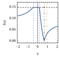 Figure 1
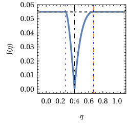 Figure 2
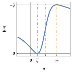 Figure 3
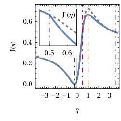 Figure 4
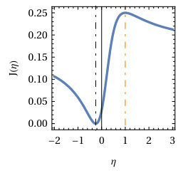 Figure 5
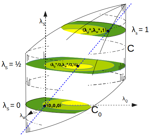 Figure 6
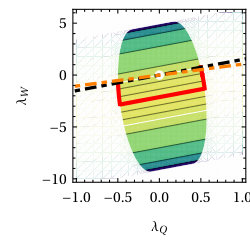 Figure 7
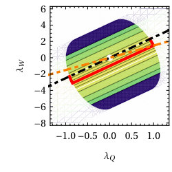 Figure 8
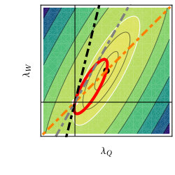 Figure 9
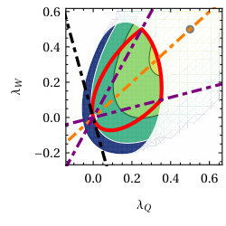 Figure 10
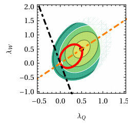 Figure 11
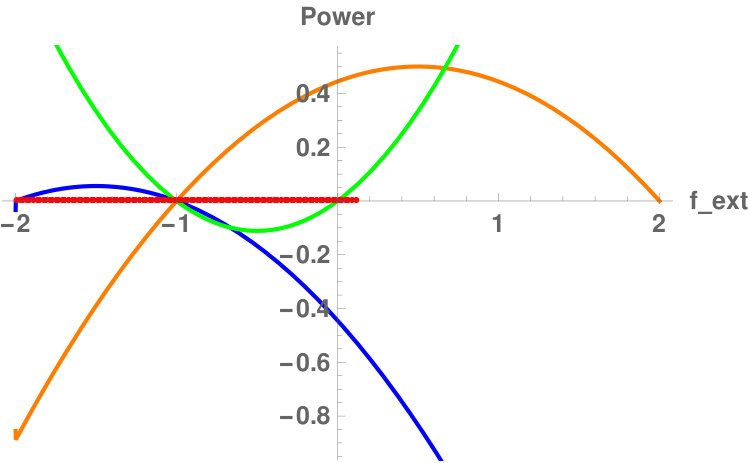 Figure 12
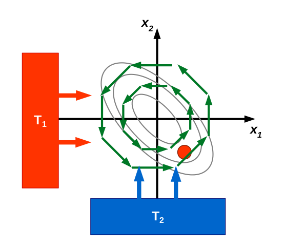 Figure 13
Peer Reviews
No public reviews on file for this paper yet. If you reviewed it on a platform where reviews are public (OpenReview, ICLR, NeurIPS, ICML), you can paste yours below so the community can read it here.
Videos
No videos yet. Explain this paper in a talk, walkthrough, or lecture? Add one.
Efficiency fluctuations in microscopic machines
Sreekanth K Manikandan
Department of Physics, Stockholm University,
SE-10691 Stockholm, Sweden.
Lennart Dabelow
Fakultät für Physik, Universität Bielefeld, 33615 Bielefeld, Germany
Ralf Eichhorn
Nordita, Royal Institute of Technology and Stockholm University, Roslagstullsbacken 23, SE-106 91 Stockholm, Sweden
Supriya Krishnamurthy
Department of Physics, Stockholm University,
SE-10691 Stockholm, Sweden.
(March 2, 2024)
Abstract
Nanoscale machines are strongly influenced by thermal fluctuations, contrary to their macroscopic counterparts. As a consequence, even the efficiency of such microscopic machines becomes a fluctuating random variable. Using geometric properties and the fluctuation theorem for the total entropy production, a “universal theory of efficiency fluctuations” at long times, for machines with a finite state space, was developed in [Verley et al., Nat. Commun. 5, 4721 (2014); Phys. Rev. E 90, 052145 (2014)]. We extend this theory to machines with an arbitrary state space. Thereby, we work out more detailed prerequisites for the “universal features” and explain under which circumstances deviations can occur. We also illustrate our findings with exact results for two non-trivial models of colloidal engines.
Understanding the functioning of machines on the micro- or nanoscale is of great interest because of their role in biological systems and their numerous technological applications Howard (2001); Parrondo and de Cisneros (2002); Benenti et al. (2017); Astumian (2012); Blickle and Bechinger (2012); Dinis et al. (2016); Krishnamurthy et al. (2016). Their small size makes this task a challenge since thermal fluctuations strongly affect their operation. As a result, average values are no longer sufficiently informative, and fluctuations in heat, work, efficiency etc. must be taken into account. Stochastic thermodynamics Seifert (2012) provides a convenient framework for analyzing such systems by extending the notions of classical (ensemble-based) thermodynamics to individual realizations of a given process.
Consider first a macroscopic heat engine operating cyclically between two reservoirs at different temperatures and performing work against an external load force. If and denote the average heat exchanged with the two reservoirs and the (average) performed work, the Second Law implies that the efficiency,
[TABLE]
is universally bounded from above by the reversible or Carnot efficiency .
The efficiency plays an equally pivotal role for microscopic machines; however, in these systems, due to thermal fluctuations, the value obtained in individual realizations can deviate significantly from the average behavior. We hence need to consider a distribution of efficiency values. Recently, in two seminal papers Verley et al. (2014a, b), Verley, Willaert, Van den Broeck, and Esposito (VWVE) developed a “universal theory of efficiency fluctuations” for machines with a finite state space. By characterizing the long-time behavior of the efficiency fluctuations in terms of their large-deviation function (see below for more details), they found that the macroscopic efficiency, defined as the ratio of average output and input powers, is the most likely and, for machines operating in a non-equilibrium steady state or under a time-symmetric periodic protocol, the reversible Carnot efficiency is the least likely one 111For machines driven asymmetrically in time, the reversible efficiency stands out as the value of at which the rate functions and for the forward and time-reversed drivings, respectively, intersect.. The VWVE theory has since been verified in numerous model systems with finite Gingrich et al. (2014); Proesmans and Van den Broeck (2015); Polettini et al. (2015a); Proesmans et al. (2015a); Esposito et al. (2015); Cuetara and Esposito (2015); Jiang et al. (2015); Agarwalla et al. (2015) but also infinite Proesmans and Van den Broeck (2015); Proesmans et al. (2015b); Agarwalla et al. (2015); Suñe and Imparato (2018) state spaces.
Nevertheless, there are a few examples of infinite state space systems at odds with the theory Park et al. (2016); Gupta (2018); Gupta and Sabhapandit (2017); Vroylandt (2018), in which the rate function fails to be smooth and/or does not exhibit a unique maximum at the reversible efficiency. A clear understanding of why some systems with infinite state space obey the “universal” theory while others do not is lacking. In this Letter, we give detailed prerequisites for when the features of the VWVE theory are found and when they are violated. In doing so, we develop an extended general theory of efficiency fluctuations, unifying the VWVE theory with deviations observed in specific models. Two examples of analytically solvable machines Gupta and Sabhapandit (2017); Filliger and Reimann (2007) serve as illustrations for our general findings.
We start by briefly summarizing the approach taken in the VWVE theory. For all systems, the total work and heat (as well as ) grow extensively with increasing operational time . For microscopic systems they also naturally fluctuate due to thermal noise, leading to a distribution for observing a heat absorption rate (the input power) and an output power with average values and . Using the theory of large deviations Touchette (2009), we can quantify the asymptotic decay of the probability towards the delta-distribution peaked at and by the large deviation or rate function ,
[TABLE]
where and . Similarly, the stochastic efficiency will tend towards the macroscopic efficiency . Again, we can describe this approach in terms of a rate function , providing an asymptotic relation for the probability distribution ,
[TABLE]
This can be extracted from the scaled cumulant generating function (sCGF) of heat and work Verley et al. (2014a, b),
[TABLE]
according to
[TABLE]
Here denotes an average over the distribution . Note that is a convex function by definition.
The relation (5) implies , where is the global minimum of . Moreover, it has the geometric interpretation, illustrated in Fig. 1: For fixed , We obtain by minimizing along the line and inverting the sign. The set of all points where the minima are attained as a function of describes a curve in the -plane (see Fig. 1) with .
Exploiting this geometrical picture, the aforementioned “universal theory” by VWVE Verley et al. (2014a, b) establishes generic properties of that are independent of system-specific details. As the main result they find that is a smooth function with a unique minimum at the macroscopic efficiency , such that , and a unique maximum at some finite efficiency . For time-symmetric driving protocols, this “least likely” efficiency coincides with the reversible efficiency Note (1), see the example in Fig. 1.
These results of the VWVE theory are based on a few assumptions, most notably: (i) The detailed fluctuation theorem Seifert (2005) for the total entropy production (where denotes the entropy change in the system itself) is valid, (ii) is a smooth function of its arguments and the fluctuation theorem implies that it has the symmetry property
[TABLE]
with and , and (iii) the minimum of is unique. The validity of (i) is by now well-established Seifert (2005, 2012). However, we will demonstrate that it does not necessarily entail the validity of the symmetry (6) for all as in (ii). Further, we discuss the case that assumption (iii) does not hold either.
While assumption (ii) appears plausible for systems with finite state space, it has been observed in certain models with infinite state space that the sCGF (4) can have a restricted domain of convergence Park et al. (2016); Gupta and Sabhapandit (2017). It has also been noticed that the symmetry property (6) need not necessarily hold Gupta and Sabhapandit (2017); van Zon and Cohen (2004a); Noh (2014a); Lee et al. (2013a); Sabhapandit (2011a); Pal and Sabhapandit (2013a). To clarify the relationship between a limited convergence domain and the symmetry relation (6), we express the sCGF in terms of the individual time-extensive and -intensive contributions to the total entropy production,
[TABLE]
Here, the term collects the time-intensive contributions to the total entropy production that depend only on the initial and final states of the system. denotes the change in internal energy, which is, according to the First Law, .
We first write down the moment-generating function (MGF) for the combined probability distribution of the individual contributions from (7),
[TABLE]
The fluctuation theorem for the total entropy production implies that has the symmetry property Lebowitz and Spohn (1999); García-García et al. (2010), . This symmetry is inherited by the three-dimensional sCGF
[TABLE]
so that
[TABLE]
The sCGF (4) of heat and work alone is the restriction of that “total” sCGF to the plane, i.e. .
As a consequence of Eq. (10) we arrive at the central observation that this restricted sCGF fulfills a “symmetry” relation of the form , instead of the relation (6). However, (6) could still be valid if were independent of . Indeed, the VWVE theory Verley et al. (2014a, b) is restricted to machines with a finite state space, in which case both, the internal energy and the system entropy , are bounded by -independent constants, implying that the dependence in (9) disappears in the limit.
However, if fluctuations of the intensive entropy production can become arbitrarily large, as is typically the case for machines with infinite state space Gupta and Sabhapandit (2017); van Zon and Cohen (2004b); Noh (2014b); Lee et al. (2013b); Verley et al. (2014c); Sabhapandit (2011b); Pal and Sabhapandit (2013b), we cannot argue that is independent of . In this case, too, the contributions drop out in Eq. (9) as wherever remains real and finite. However, in contrast to the finite state-space case, the limited domain of convergence of will in general depend on . As a consequence of the fluctuation theorem symmetry obeyed by , is symmetric about the point . Therefore, the restriction of to the plane satisfies a symmetry property like (6), but the domain of convergence of at will in general not obey this symmetry, and hence neither will . This situation is illustrated in Fig. 2.
What are the consequences of the limited domain of convergence and its lack of symmetry for the large deviation function ? The answer depends on whether the minimizing curve is completely contained inside or whether it touches or hits the boundary of . We illustrate this difference using the isothermal work-to-work converter from Ref. Gupta and Sabhapandit (2017), which exhibits both of these cases depending on the amplitude ratio of work and load forces. This machine consists of a Brownian particle in contact with a single heat bath at temperature and two additional white-noise forces, interpreted as a load and drive force, respectively. Identifying the work done by the drive force with and the work done by the load force with , we can calculate the sCGF exactly, and from that the curve and rate function (see Gupta and Sabhapandit (2017) and the Supplemental Material sup which includes references Gärtner (1977); Ellis (1984) for details).
In the first case, when lies completely inside , the existence of singular points for is irrelevant, resulting in a that has exactly the properties and “universal shape” predicted by the VWVE theory (see the top panels in Fig. 3). In particular, the reversible efficiency is still least likely, because the global minimum of is still attained at the point despite the “asymmetry” of . By contrast, in the second case, takes its minimal value on the boundary of (lower left panel in Fig. 3). The minimizing curve thus follows the boundary of for some range of values and becomes non-smooth at the points where the path transitions from the interior to the boundary and vice versa, leading to kinks in the first derivative of (lower right panel in Fig. 3). We conclude that the appearance of cutoffs in can lead to discontinuities or “kinks” in or its derivatives. In general (see also sup ), is a smooth function of if and only if is smooth along the curve . Note that in the second example of Fig. 3 (lower panels), the least likely efficiency is still , even though does not obey the symmetry (6). However, this need not be the case in general since the minimal -value need no longer be located on the line .
Next, we investigate the situation when assumption (iii) fails to hold and the global minimum of is not unique but rather degenerate 222Degeneracy in in systems with both tight coupling and dynamical phase transitions has been investigated in Vroylandt (2018), i.e. there exist multiple points in the set . Due to the convexity of , this set will be a connected region in the -plane. Then assumes its maximal value for all for which the line intersects the region , leading to a plateau of degenerate maxima. Presumably, such a scenario could also occur in systems with finite state space. The reversible efficiency is one of these maximizing efficiencies if and only if the line intersects the region within the domain of convergence (see also sup ).
We illustrate this situation with the example of the “Brownian gyrator” Filliger and Reimann (2007); Pietzonka and Seifert (2018). This heat engine consists of a colloidal particle in two dimensions, immersed in a fluid environment and experiencing thermal fluctuations of different intensity along two perpendicular directions (temperatures and , friction coefficients and ; see Argun et al. (2017); Chiang et al. (2017) for experimental realizations). The particle is trapped in a harmonic potential whose principal axes with stiffnesses and are rotated by an angle with respect to the preferred axes of the heat baths. As a consequence, the particle experiences a net torque letting it rotate around the origin on average Filliger and Reimann (2007). Applying a linear “load torque” with slope , the system operates as a stationary, heat engine Pietzonka and Seifert (2018) (see also sup for details). The resulting sCGF and rate function can be computed exactly using path-integral techniques Manikandan and Krishnamurthy (2017, 2018) ( see also sup , which includes references Onsager and Machlup (1953); Machlup and Onsager (1953); Chernyak et al. (2006); Kirsten and McKane (2003) ) and are shown for two different configurations in Fig. 4. In this system, the degenerate minimum of results from becoming a function of only within the domain of convergence due to tight coupling between work and heat Polettini et al. (2015a). The iso-contours of , one of them being the set , are therefore parallel lines with slope (see left panels of Fig. 4). The resulting plateaus for are visible in the right panels. For the configuration in the top panels, the region intersects the -axis, so that the plateau of extends to . Moreover, in this configuration the line intersects , so that the Carnot efficiency lies at the edge of the plateau of degenerate maxima of . In contrast, for the second configuration in the lower panels, does not intersect the -axis and the plateau is restricted to a finite region of values. Furthermore, this plateau does not contain the Carnot efficiency . We note that in both cases has kinks resulting from the minimizing curve hitting the boundary of the domain of convergence . A similar efficiency distribution has also been obtained in Park et al. (2016) for a closely related model.
In conclusion, we have extended the VWVE theory of efficiency fluctuations by including three crucial insights: First, the domain of convergence of determines if the fluctuation theorem symmetry (6) holds or not. The resulting cutoffs lead to a differing from the VWVE theory, if and only if is non-smooth along the curve . Since depends on the boundary terms, this opens up possibilities to fine-tune initial conditions to change and, for example, minimize fluctuations around the macroscopic efficiency. Secondly, can have degenerate minima, typically leading to a plateau of maximal values for . Finally, the symmetry (6) is sufficient, but not necessary for the least likeliness of the Carnot efficiency . On the other hand, is no longer least likely in general. Our results are obtained from generic features of the sCGF and incorporate as special cases the VWVE theory as well as exceptions found in specific models. Exact solutions for two non-trivial models support our observations.
Acknowledgements.
Acknowledgements. LD acknowledges funding by the Deutsche Forschungsgemeinschaft within the Research Unit FOR 2692 under Grant No. 397303734 as well as by the Stiftung der Deutschen Wirtschaft. LD also thanks Nordita for the hospitality and support during an internship in 2016. RE acknowledges financial support from the Swedish Research Council (Vetenskapsrådet) under the grant No. 2016-05412.
Supplemental material
This document provides further details of the calculations behind the results presented in the manuscript “Efficiency fluctuations in microscopic machines”. In the first section, we further elaborate the relationship between properties of the scaled cumulant generating function of heat and work and properties of the efficiency rate function . In the second section, we summarize the essential findings (relevant for our analysis) of Ref. Gupta and Sabhapandit (2017) about the isothermal work-to-work converter used as an illustrative example in the main text. In the third section, we introduce the Brownian gyrator model, which served as a second illustrative example in the main text, and present details on the derivation of its scaled cumulant generating function of heat and work.
Relation between properties of and properties of
In this section, we formalize how certain prerequisites for the scaled cumulant generating function (sCGF) of heat and work lead to properties of the efficiency rate function , namely, smoothness, the least likely efficiency and plateaus.
Before we turn to the specific observations from the main text, we collect a few basic properties of the sCGF . By definition (see Eq. (4) in the main text ), is a convex function, notably meaning that the sublevel sets
[TABLE]
are convex. Moreover, it satisfies the normalization condition . As is obtained from by minimizing along lines through the origin and inverting the sign (see Eq. (5) in the main text), this immediately implies . It also implies that the curve is contained in the sublevel set .
Furthermore, for large deviation theory to be applicable to the problem at all, we need that the rate function , defined via Eq. (2) from the main paper, is well-defined and, in particular, has a finite value. This in turn implies, according to the Gärtner-Ellis theorem Gärtner (1977); Ellis (1984); Touchette (2009) , that is bounded from below, so that there is a value with for all , . All these properties will be taken for granted in the following.
Smoothness
As argued in the main text, is a smooth function of if and only if is smooth along the curve . This follows immediately from the definition of [see also Eq. (5) from the main paper] and from the definition of , implying . However, this criterion is not very “practical” because it generally becomes quite complicated to determine the curve in the presence of singular points for . A more accessible (albeit weaker) characterization is as follows:
If the global minimum of is unique and there exists an open region with such that is smooth in and the Hessian matrix of is positive definite in , then is smooth.
This provides a sufficient (but not necessary) condition on for to be smooth. To prove this, assume that is smooth in some open region containing the sublevel set . Moreover, assume that the Hessian matrix of is positive definite on , implying that the function is strictly convex on . Smoothness means that is infinitely differentiable for all . For every , denote by a point with that minimizes Eq. (5), i.e. . As observed above, for all , so that . Obviously, , meaning that the function is determined by the values of on the curve with . It suffices to show that this mapping is smooth. The smoothness of in then implies that is smooth as well.
Smoothness and convexity of imply that the line is tangent to the iso-contour in the point . Due to smoothness, the iso-contour is , the boundary of the sublevel set from Eq. (11). Since is strictly convex, so are the sublevel sets , and consequently the point is unique for all . The fact that the line of efficiency is tangent to an iso-contour of in means that the ray vector of the line is orthogonal to the gradient of in . Thus
[TABLE]
This relation along with implicitly defines as a function of . More precisely, we consider the function
[TABLE]
Assume that we have a particular solution of (12) for some given , so that . Due to the assumed positive definiteness of the Hessian matrix of , we have
[TABLE]
By the implicit function theorem, there exists a function on an open interval with and such that for all . Moreover, this function is of the same differentiability class as . Put differently, the parameter function implicitly defined by Eq. (12) is well-defined and smooth in . As this holds everywhere in , we conclude that and thus is smooth.
Least likely efficiency
The “least likely” efficiency, i.e. the value that maximizes , is directly related to the global minimum of . Indeed, if assumes its minimal value at , then will become maximal for by Eq. (5). As observed in the main text and investigated in more detail in the next section of this Supplemental Material, the global minimum of need not be unique in general, so that can have a degenerate maximum (“plateau”) as well. In any case, the reversible efficiency maximizes if and only if the global minimum of lies on the line .
As observed in Refs. Verley et al. (2014a, b), the symmetry property Eq. (6) provides a sufficient (but not necessary) condition for the least likeliness of the reversible efficiency . Indeed, if Eq. (6) holds then the iso-contour lines of are invariant under reflection through the point . By convexity, must therefore attain its minimal value in the reflection point, so that . Hence assumes the maximum possible value for the line with slope .
Plateau
We have illustrated in the main text that there could be cases where the global maximum of is not unique, meaning that there may be an entire “plateau region” where assumes its maximal value. As stated in the main text,
The maximum of is unique if and only if all minimizing points of lie on a line through the origin with fixed slope .
Below, we elaborate on this feature.
Let us first assume that there exist with and , so that the minimizing points of do not lie on a single line through the origin. (Recall that denotes the set of all with , c.f. Eq. (11)). The latter condition ensures that the slopes of the lines connecting the origin with and , respectively, are different, meaning that . But since both lines cut through the global minimum, it follows that , establishing the degeneracy of . Moreover, by convexity of , all lines with slopes between and will also cross the global minimum, so that all plateau efficiencies are connected. In other words, there cannot be two separate plateaus in disjoint intervals of the extended(!) real line . (However, the plateau may be connected through the point , corresponding to the line .) We remark that the emergence of plateaus need not necessarily be due to “tight coupling” as in the Brownian gyrator example presented in the main text (Fig.4 ). The tight coupling case, where is a special case exhibiting a degenerate global minimum.
To show the converse direction, assume that there is a unique such that all points with satisfy . Then all such points lie on the line , while for all and all , . Hence has a unique maximum at .
Example 1: Isothermal work-to-work converter engine Gupta and Sabhapandit (2017)
In this section, we provide details about the example of an isothermal work-to-work converter by briefly summarizing the main results from Ref. Gupta and Sabhapandit (2017) that are relevant for our purposes.
The model consists of a Brownian particle of mass in a fluid environment at temperature with instantaneous velocity . By the fluctuation-dissipation theorem, the coupling to the heat bath gives rise to a fluctuating force as well as a frictional force , where is the friction coefficient and is a Gaussian white-noise process with and . In addition, the particle is subject to two more fluctuating forces and with Gaussian white-noise statistics, independent of each other as well as of the thermal noise, i.e. and . The resulting equation of motion thus reads
[TABLE]
The relative strength of the three fluctuating forces with respect to each other is parameterized by the positive parameters and such that and . The force and are interpreted as a load and drive force, respectively. The work done by them is given by
[TABLE]
Translated to the setting in the main text, we thus identify with and with . The resulting moment-generating function for and was found in Ref. Gupta and Sabhapandit (2017) to satisfy the asymptotic relation
[TABLE]
where
[TABLE]
From this, the scaled cumulant generating function can be extracted straightforwardly.
I Example 2: Brownian gyrator
In this section, we give a detailed definition of the Brownian gyrator model adapted from Ref. Filliger and Reimann (2007) and provide the exact solution of its scaled cumulant generating function .
The model consists of a Brownian particle in two dimensions at position , sketched in Fig. 5. The particle is immersed in a fluid environment and simultaneously coupled to two (effective) heat baths at different temperatures that only act in the and directions, respectively. For example, the colder temperature may be the temperature of the surrounding fluid, while there are additional fluctuations in the directions due to external fields or an irradiating heat bath leading to a higher effective temperature Filliger and Reimann (2007), see Argun et al. (2017) for an experimental realization or Chiang et al. (2017) for an equivalent electric circuit system.
By the fluctuation-dissipation theorem, the coupling to the environments leads, in both directions, to fluctuating forces on the one hand and frictional forces on the other hand, where are the respective friction coefficients and are independent Gaussian white-noise processes with and . The particle is confined by a parabolic potential with stiffnesses and along its principal axes, which are tilted by an angle with respect to the coordinate axes:
[TABLE]
Due to the asymmetry of the thermal and restoring forces (for , , and , ), the particle reaches a non-equilibrium steady state and rotates around the origin on average Filliger and Reimann (2007). It thereby exerts a torque on the environment and can thus work as a microscopic heat engine. To quantify the work done, we generalize the model studied in Filliger and Reimann (2007) by introducing an additional external force (see also Pietzonka and Seifert (2018))
[TABLE]
is the two dimensional antisymmetric tensor. In the overdamped limit the dynamics of the Brownian Gyrator is then described by the equations of motion
[TABLE]
where
[TABLE]
For the range of parameter values where the matrix A is positive definite, the system reaches a steady state with probability distribution Argun et al. (2017)
[TABLE]
where is obtained as a solution of
[TABLE]
The work done by the external load force as well as the heat taken from the hot reservoir over a process of time duration can be obtained using the standard definitions of stochastic thermodynamics as
[TABLE]
with
[TABLE]
In Fig. 6, we display the resulting average input and output powers , , and as a function of the load amplitude for a certain choice of parameters. It illustrates that the system indeed works as a heat engine for moderate loads with .
Now using the path integral formalism, the moment generating function (MGF) of and at arbitrary times can be obtained as
[TABLE]
where
[TABLE]
denotes the Onsager-Machlup path weight Onsager and Machlup (1953); Machlup and Onsager (1953); Chernyak et al. (2006). Since all the terms in the exponent of the RHS of Eq. (41) are quadratic in and their derivatives, we can write this as Manikandan and Krishnamurthy (2017)
[TABLE]
Here the operator is a matrix with differential operators as its entries Kirsten and McKane (2003), and the determinants that appear in Eq. (44) are functional determinants. For our problem, it can be shown that the matrix has the form
[TABLE]
where
[TABLE]
Then the determinant ratio that appears in Eq. (44) can be computed using a technique described in Kirsten and McKane (2003) and recently used in Manikandan and Krishnamurthy (2017), which is based on the spectral- functions of Sturm-Liouville type operators. Applying this method to the model at hand, it can be shown that this ratio can be obtained in terms of a characteristic polynomial function as
[TABLE]
Here is the matrix of independent and suitably normalized fundamental solutions of the homogeneous equation ,
[TABLE]
and and contain information about the boundary conditions from Eq. (43), for which we require
[TABLE]
A derivation of Eq. (49), applicable to a class of driven Langevin systems with quadratic actions, is given in Manikandan and Krishnamurthy (2017). We stress that the expression given in Eq. (49) is valid within the domain for which the operator doesn’t have negative eigenvalues. The MGF is not convergent outside this domain.
For the Brownian gyrator problem, we obtain the four independent solutions as
[TABLE]
The matrices and are given by
[TABLE]
Using these, the MGF can be computed exactly using Eq. (49). Notice that the solution is valid for arbitrary time . Various interesting finite time aspects of this solution will be discussed in a future publication. Here we focus on the large time limit, where the leading order form of the MGF is given by
[TABLE]
Using the exact solution obtained from Eq. (49), the large time functional form given above can be obtained by performing an asymptotic expansion using Mathematica. We provide here the exact functional forms for the completion of the discussion:
[TABLE]
In terms of the function defined as
[TABLE]
we obtain
[TABLE]
The reference list from the paper itself. Each links out to its DOI / PubMed record.
- 1Howard (2001) Jonathon Howard, Mechanics of Motor Proteins and the Cytoskeleton (Oxford University Press, 2001).
- 2Parrondo and de Cisneros (2002) JMR Parrondo and B Jiménez de Cisneros, “Energetics of Brownian motors: a review,” Applied Physics A 75 , 179–191 (2002).
- 3Benenti et al. (2017) Giuliano Benenti, Giulio Casati, Keiji Saito, and Robert S Whitney, “Fundamental aspects of steady-state conversion of heat to work at the nanoscale,” Phys. Rep. 694 , 1–124 (2017).
- 4Astumian (2012) R Dean Astumian, “Microscopic reversibility as the organizing principle of molecular machines,” Nat. Nanotechnol. 7 , 684 (2012).
- 5Blickle and Bechinger (2012) Valentin Blickle and Clemens Bechinger, “Realization of a micrometre-sized stochastic heat engine,” Nat. Phys. 8 , 143 (2012).
- 6Dinis et al. (2016) L Dinis, I A Martínez, É Roldán, J M R Parrondo, and R A Rica, “Thermodynamics at the microscale: from effective heating to the brownian carnot engine,” Journal of Statistical Mechanics: Theory and Experiment 2016 , 054003 (2016) .
- 7Krishnamurthy et al. (2016) Sudeesh Krishnamurthy, Subho Ghosh, Dipankar Chatterji, Rajesh Ganapathy, and A. K. Sood, “A micrometre-sized heat engine operating between bacterial reservoirs,” Nature Physics 12 , 1134 (2016) . · doi ↗
- 8Seifert (2012) Udo Seifert, “Stochastic thermodynamics, fluctuation theorems and molecular machines,” Rep. Prog. Phys. 75 , 126001 (2012) .