Score-based Tests for Explaining Upper-Level Heterogeneity in Linear Mixed Models
Ting Wang, Edgar C. Merkle, Joaquin A. Anguera, Brandon M. Turner

TL;DR
This paper introduces score-based tests to detect and explain heterogeneity in variance components within linear mixed models, helping researchers identify clusters with differing variances and improve fixed effect inference.
Contribution
The study extends score-based tests to linear mixed models, providing a systematic method to detect variance heterogeneity and identify specific clusters with differing variances.
Findings
Score-based tests effectively detect heterogeneity in variance components.
The tests can identify specific clusters with differing variances.
Application to empirical data demonstrates practical utility.
Abstract
Cross-level interactions among fixed effects in linear mixed models (also known as multilevel models) are often complicated by the variances stemming from random effects and residuals. When these variances change across clusters, tests of fixed effects (including cross-level interaction terms) are subject to inflated Type I or Type II error. While the impact of variance change/heterogeneity has been noticed in the literature, few methods have been proposed to detect this heterogeneity in a simple, systematic way. In addition, when heterogeneity among clusters is detected, researchers often wish to know which clusters' variances differed from the others. In this study, we utilize a recently-proposed family of score-based tests to distinguish between cross-level interactions and heterogeneity in variance components, also providing information about specific clusters that exhibit…
Click any figure to enlarge with its caption.
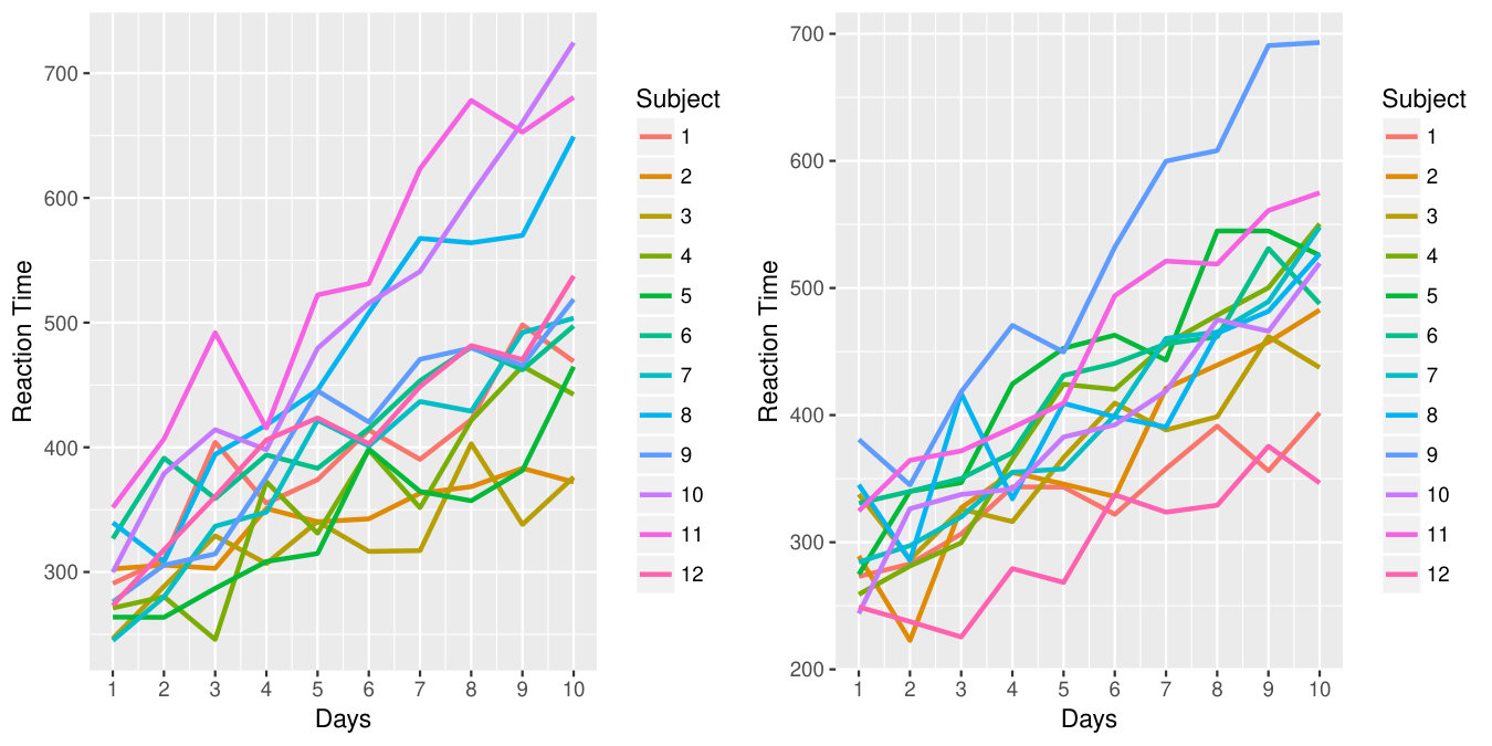 Figure 1
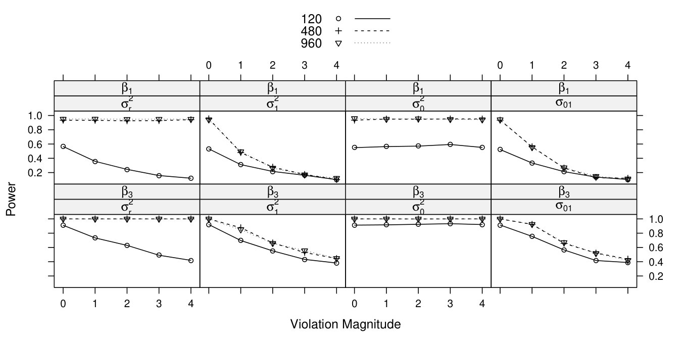 Figure 2
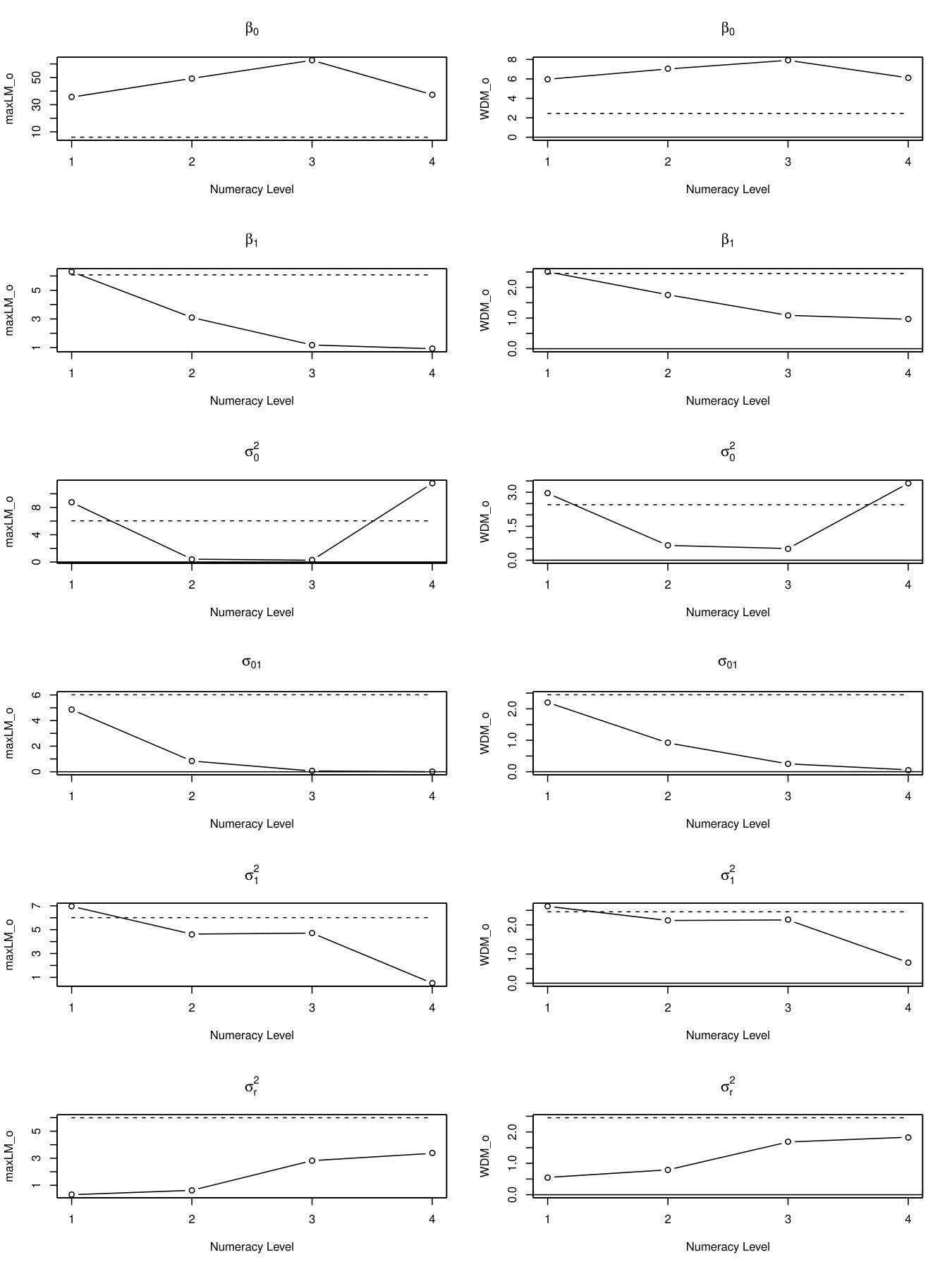 Figure 3
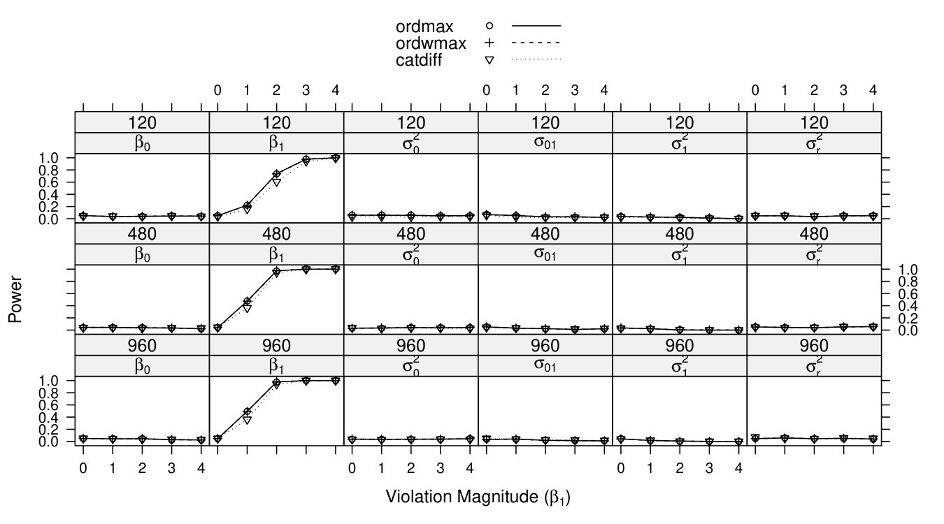 Figure 4
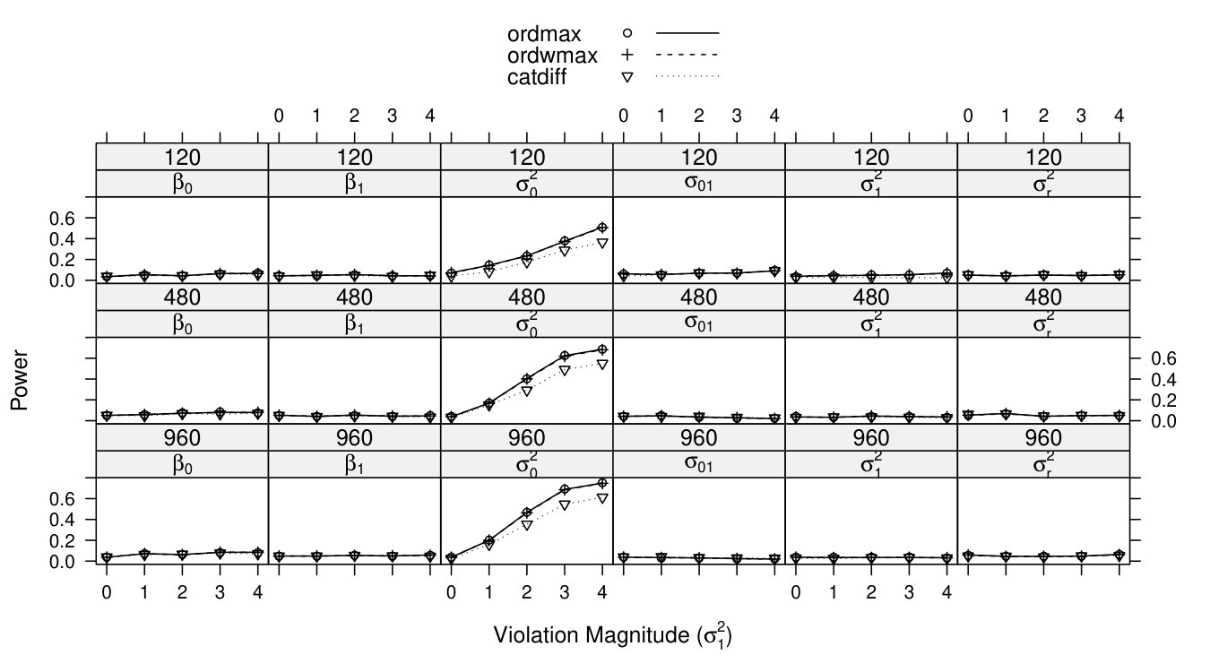 Figure 5
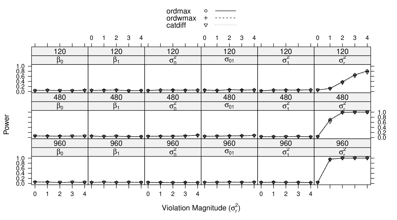 Figure 6
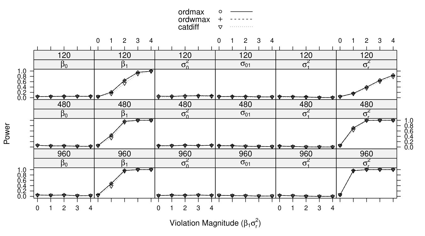 Figure 7
Peer Reviews
No public reviews on file for this paper yet. If you reviewed it on a platform where reviews are public (OpenReview, ICLR, NeurIPS, ICML), you can paste yours below so the community can read it here.
Videos
No videos yet. Explain this paper in a talk, walkthrough, or lecture? Add one.
Taxonomy
TopicsMental Health Research Topics · Advanced Statistical Modeling Techniques · Statistical Methods and Bayesian Inference
\setremarkmarkup
(#2)
\fourauthorsTing WangEdgar C. MerkleJoaquin A. Anguera Brandon M. Turner \fouraffiliationsThe American Board of Anesthesiology University of Missouri University of California, San Francisco The Ohio State University
Score-based Tests for Detecting Heterogeneity in Linear Mixed Models
Abstract
Cross-level interactions among fixed effects in linear mixed models (also known as multilevel models) can be complicated by heterogeneity stemming from random effects and residuals. When heterogeneity is present, tests of fixed effects (including cross-level interaction terms) are subject to inflated Type I or Type II error. While the impact of variance change/heterogeneity has been noticed in the literature, few methods have been proposed to detect this heterogeneity in a simple, systematic way. In addition, when heterogeneity among clusters is detected, researchers often wish to know which clusters’ variances differed from the others. In this study, we utilize a recently-proposed family of score-based tests to distinguish between cross-level interactions and heterogeneity in variance components, also providing information about specific clusters that exhibit heterogeneity. These score-based tests only require estimation of the null model (when variance homogeneity is assumed to hold), and they have been previously applied to psychometric models to detect measurement invariance. In this paper, we extend the tests to linear mixed models, allowing us to use the tests to differentiate between interaction and heterogeneity. We detail the tests’ implementation and performance via simulation, provide an empirical example of the tests’ use in practice, and provide code illustrating the tests’ general application.
Acknowledgements.
This work was supported by National Science Foundation grants SES-1061334 and 1460719. Correspondence to Ting Wang. Email: [email protected]
\rightheaderDetecting heterogeneity in mixed models
1 Introduction
Cross-level interactions are often of interest for researchers adopting linear mixed models (also known as multilevel models or hierarchical linear models), which specifically refers to the interaction between a lower-level (level 1) covariate and a upper-level (level 2) covariate. For example, in a cross-sectional study of students within schools, we might observe a cross-level interaction between students’ cognitive ability (level 1) and school climate (level 2). In a longitudinal study of repeated observations within participants, we might note a cross-level interaction between time (level 1) and participant socioeconomic status (level 2). However, the estimation and testing of cross-level interactions in linear mixed models (LMMs) is often complicated by the multiple variance terms in the model. For example, when a cross-level interaction exists, it may not be detected due to heterogeneity in a random effect variance or in a residual variance (?, ?). If this heterogeneity is not accounted for, it can lead to biased standard error estimates (?, ?, ?) and incorrect significance tests for fixed parameters (?, ?).
Heterogeneous (co-)variances often occur in longitudinal studies, where the heterogeneity in variance/covariance is observed across individuals. For example, recent ecological momentary assessment (EMA) studies have shown that substantial heterogeneity exists across individuals in the variance and covariance of emotional states over time (?, ?, ?, ?, ?). A similar phenomenon occurs in education research, where it is of interest to model student achievement over time (?, ?). This heterogeneity is often due to unobserved covariates or to confounding with other covariates (such as time; ?, ?, ?); issues that are inevitable in many applied scenarios (?, ?). Hence, it is important to develop accessible methods to detect heterogeneity in the multiple variance parameters observed in mixed models.
Several previous methods test for heterogeneity by building it into the model and using a likelihood ratio (LR) test or Kolmogorov-Smirnov test (?, ?, ?, ?). The LR test can be used when heterogeneity can be explained by observed variables. For example, semtree (?, ?), longRpart2 (?, ?) and ? (?) all utilize a series of LR test to detect potential split point(s) along auxiliary variables. However, this test can be cumbersome when the variable has many categories, and it can be sub-optimal when the variable is ordinal or continuous. In contrast, the Kolmogorov-Smirnov test utilizes a mixture model framework, and checks the correct number of mixture components in an omnibus goodness-of-fit test. However, as shown by ? (?), this approach is subject to low power, even decreasing to zero when the residual variance is large.
In this paper, we aim to extend a family of score-based tests (e.g., ?, ?, ?) to the study of heterogeneity in linear mixed models. These tests have been previously applied to detect measurement invariance in factor analysis (?, ?, ?, ?) and in models from item response theory (IRT; e.g., ?, ?, ?). This study serves as a novel application of the tests in the context of LMM by providing a unified new approach to differentiate heterogeneity in variance components (either random effects or residual) from cross-level interactions. From a technical perspective, this study differs from the previous measurement invariance studies in that the casewise scores are not i.i.d. any more by definition, since the observations within the same cluster are correlated. In addition, we focus on heterogeneity in both fixed parameters and variance/covariance parameters, whereas the related approach of ? (?) has tested only for changes in fixed parameters while maintaining homogeneity in variance and covariance parameters. We also discuss graphical methods associated with the tests, which can be helpful for identifying clusters that exhibit similar variance estimates. In the following section, we provide a brief overview of the score-based tests’ generalizations to linear mixed models. Next, we report on the results of a simulation to examine the tests’ abilities in the context of linear mixed models. Finally, we provide an empirical example with illustrating code and discuss the tests’ future generalizations.
2 Linear Mixed Model
The linear mixed model (LMM) can be expressed in both conditional and marginal forms. The former facilitates theoretical understanding, and the latter simplifies the computational expression. We will detail these two expressions in the following sections, focusing on a two-level model where individual observations are nested within a series of clusters.
2.1 Conditional Expression
The conditional version of the LMM can be written as
[TABLE]
where is the observed data vector for the th cluster, (so that the level 1 sample size is given as ); is an matrix of fixed covariates; is the fixed effect vector of length ; is an design matrix of random effects; and is the random effect vector of length .
The vector is assumed to follow a normal distribution with mean and covariance matrix , where is a matrix composed of variances/covariances for random effect parameters. The residual covariance matrix, , is the product of the residual variance and an identity matrix of dimension . Later, the matrix will include residuals across all clusters, so the identity matrix is of dimension .
Based on the notations above, the following notation is used to represent data and parameters across all clusters in the data.
[TABLE]
where is the Kronecker product.
Finally, we define to be a vector of length , containing all variance/covariance parameters (including those of the random effects and the residual). This implies that the matrix has unique elements. For example, in a model with two random effects that are allowed to covary, is a vector of length 4 (i.e., ). The first three elements correspond to the unique entries of , which are commonly expressed as , , and . The last component is then the residual variance .
2.2 Marginal Expression
Based on Equations 1, 2, and 3, the marginal distribution of the LMM is
[TABLE]
where
[TABLE]
where denotes a matrix transpose. By using the combined notation from Equation (4) to Equation (7), we can further define as
[TABLE]
Thus, Equation (9) can be rewritten as:
[TABLE]
From Equation (13), we can perceive the LMM as a regular linear model with correlated residual variance . From this perspective one can easily deduce that heterogeneity in has little impact on the estimate of , because is still equal to , but can have a large impact on the significance test of (?, ?). We will illustrate this issue in the following section.
3 Problems Stemming from Heterogeneity
We now illustrate implications of heterogeneity via both theoretical results and simulation.
3.1 Theoretical Demonstration
The variance-covariance matrix w.r.t. the fixed parameter corresponds to the inverse of the model’s Fisher information, the relevant part of which can be expressed as (e.g., ?, ?):
[TABLE]
The standard error of fixed parameters, , is then the square root of the diagonal elements of . This shows that directly contributes to the fixed parameters’ standard errors, which in turn influences the fixed parameters’ test statistics. With the under/over-estimates of , the t-statistic will be larger/smaller than it should be. Generally one can expect that the increasing of results in Type II error whereas decreasing of leads to Type I error. In practice, the former happens more often. ? (?) conducted a series of Monte Carlo simulations and found underspecification and misspecification of result in overestimation of , which lead to lower statistical power in significance tests of the fixed parameters. Although their simulations only examined main effects, one can expect similar results for interaction effects. We illustrate this issue in the next section.
3.2 Data Demonstration
In this section, we specifically illustrate how the change (increase) in could impact the significance of fixed parameters by using artificial data similar to the sleepstudy data (?, ?) included in lme4. This dataset includes subjects participating in a sleep deprivation study, where each subject’s reaction time (RT) 111Strictly speaking, the response variable should be log(RT) to have a meaningful infinity support. was monitored for consecutive days. The reaction times are nested within subject and continuous in measurement. Then we fit a model with day of measurement (“Days”) as the covariate, including random intercepts and slopes that are allowed to covary. This leads to a model whose free parameters include: the fixed intercept and slope and ; the random variance and covariances , , and ; and the residual variance . To illustrate the impact of heterogeneity on cross-level interactions, we also simulate an ordinal variable with four levels loosely called Cognitive Ability (CA), with its own main effect coefficient as and its interaction effect Cognitive Ability (CA) Days coefficient as . In the simulation, we focus on the significance test results of and . The true values were set to be and , respectively, with both far different from [math]. The random effect variance/covariance and residual variance were set to be the same as the estimates obtained from the sleepstudy data. This leads to the model displayed from Equation (17) to Equation (21).
[TABLE]
From Equation (10), it can be observed that changes in can come from either , which is composed of between-subjects variance parameters and , or the residual variance . We generated data so that changed with each of these four parameters, including the between subjects intercept variance , slope variance , covariance and residual variance , along with different sample sizes as small (), medium () and large (). Changes in these variance parameters began at cognitive ability level 2 and were consistent thereafter. Participants below cognitive ability level 2 deviated from participants at or above level 2 by times the parameters’ asymptotic standard errors (scaled by ), with . To obtain the asymptotic standard error, we first fit a model under the above parameter settings but with a large sample size, e.g. ; then the asymptotic standard error can be extracted by taking the square root of the diagonal elements of the variance covariance matrix. The replication code for obtaining asymptotic standard error used throughout this paper is provided in the supplementary material.
The magnitude of change is reflected in . When is 0, it represents homogeneity in the corresponding parameter, which serves as the baseline; when is greater than 0, it represents heterogeneity in (increasing with Cognitive Ability in this example), with larger indicating more severe heterogeneity. One example of data with and without heterogeneity is displayed in Figure 1. In the left panel, data were generated without heterogeneity in random slope (); whereas in the right panel data were generated with heterogeneity in random slope as large as . Within each panel, the subjects 1-6 denoted with gray lines have cognitive ability equal to or less than 2, whereas subject 7-12 denoted with yellow lines have cognitive ability greater than 2. Without the impact of variance heterogeneity (left panel), it is easy to observe that the RT has a positive relation with Days (), and this relation differ for subjects with different cognitive abilities . However, these relations are difficult to see under the impact of variance change (right panel). Unfortunately, the real data often look more similar to the right panel, with no obvious relations to be detected even if the generating fixed parameters are actually exactly the same as the left panel. To formally examine the impact of heterogeneity, we computed the percentage of significant fixed parameters related to “Days” ( and ) among replications in each condition.
The full simulation results for and are demonstrated in Figure 2, with the panel titles first indicating the tested parameter and then indicating the heterogeneous parameter, and the y-axis representing power (using ). In general, when sample size is medium or large, increasing heterogeneity in the slope variance or covariance reduces power for both the main effect and interaction effect. Heterogeneity in the residual variance or intercept variance does not impact power for or , because they can be compensated for during estimation (?, ?). That is to say, when the intercept variance (or residual variance) increases, the residual variance (or intercept variance) estimate will decrease to compensate for the change, leading to the diagonal of being unchanged. This compensation effect exists because the intercept covariate in the random effect design matrix () is all , so that the intercept and residual variance contribute equally to the diagonal of .
When sample size is small (), power is generally lower in all scenarios. In addition, greater heterogeneity in the residual variance also leads to lower power, which might be due to the fact that heterogeneity combined with small sample size is more likely to result in unstable variance/covariance estimates, or even convergence issues.
Overall, however, failing to account for the upward changes in would generally result in Type II error. Although it is important to systematically monitor heterogeneity in variance components, it is also plausible that a fixed parameter indeed changes according to another variable (e.g., that an interaction exists). Ideally, there would exist a statistical test that can differentiate between these two kinds of changes. In the next section, we will introduce a score-based family of statistical tests that can fulfill this need.
4 Score-based Tests
In this section, we will introduce the score-based test as applied to the framework of LMM. This introduction draws on LMM results described by ? (?) and is related to tests described by, e.g., ? (?), ? (?), and ? (?).
4.1 Scores
Based on the marginal model expression shown in Equation (13), the log likelihood of the LMM can be expressed as:
[TABLE]
Scores, denoted in this paper, are based on the first partial derivatives of w.r.t. . The scores involve these partial derivatives evaluated for each observation , where = , and they can be roughly viewed as a residual: values close to 0 imply that the model provides a good fit to case with respect to a specific parameter, and values far from 0 imply the opposite.
The model gradient is equal to the sum of scores across all individuals and clusters:
[TABLE]
where represents the first derivative within cluster , which can be expressed as the sum of the casewise score belonging to cluster . For LMMs, the function w.r.t. and can be expressed as the th component of the vectors or as the th row of the matrix (if contains multiple components):
[TABLE]
where represents the Hadamard product (component-wise multiplication). Further detail on these derivations can be found in ? (?), ? (?), and ? (?).
These equations provide scores for each observation , and we can construct the clusterwise scores by summing scores within each cluster. In situations with one grouping (clustering) variable, the clusterwise scores can be obtained from a fitted lme4 model via R package merDeriv (?, ?).
4.2 Statistics
As applied to the LMMs considered here, score-based tests can be used to study heterogeneity that is potentially explained by an auxiliary variable ; for example, in the data demonstration considered earlier, the auxiliary variable could have been Cognitive Ability. Because the scores can be viewed as a type of residual, the score-based tests basically help us judge whether the residual magnitudes are associated with . Because we have unique scores for each model parameter, we can also obtain information about where heterogeneity occurs.
Statistically, the tests considered here can be viewed as generalizations of the Lagrange multiplier test. The tests are based on a cumulative sum of scores, where the order of accumulation is determined by . If there is no heterogeneity explained by , then this cumulative sum should fluctuate around zero. Otherwise, the cumulative sum would systematically diverge from zero.
To formalize these ideas, we first define the (scaled) cumulative sum of the ordered scores. This can be written as
[TABLE]
where is an estimate of the information matrix, is the integer part of (i.e., a floor operator), and reflects the cluster with the -th smallest value of the auxiliary variable . While the above equation is written in general form, we can restrict the value of in finite samples to the set . We focus on how the cumulative sum fluctuates as more clusters’ scores are added to it, e.g., starting with the person of lowest cognitive ability and ending with the person of highest cognitive ability. The summation is premultiplied by an estimate of the inverse square root of the information matrix, which serves to decorrelate the fluctuation processes associated with model parameters. For LMMs, can be written as expected information matrix (e.g., ?, ?):
[TABLE]
4.3 Score-based tests statistics
To obtain an official test statistic, we must summarize the behavior of the cumulative sum in a scalar. Multiple summaries are available, leading to multiple tests of the same hypothesis. For example, one could take the absolute maximum that the cumulative sum attains for any parameter of interest, resulting in a double max statistic (the maximum is taken across parameters and clusters entering into the cumulative sum). Alternatively, one could sum the (squared) cumulative sum across parameters of interest and take the maximum or the average across clusters, resulting in a maximum Lagrange multiplier statistic and Cramér-von Mises statistic, respectively (see ?, ?, for further discussion). These statistics are given by
[TABLE]
For an ordinal auxiliary variable with levels, we can modify the statistics above so that the maximum is only considered after all clusters at the same level of have entered the summation. This leads to test statistics that are especially sensitive to heterogeneity that is monotonic with (?, ?). Formally, we define to be the empirical, cumulative proportions of clusters observed at the first levels of . The modified statistics are then given by
[TABLE]
where .
Finally, if the auxiliary variable is only nominal/categorical, the cumulative sums of scores can be used to obtain a Lagrange multiplier statistic. This test statistic can be formally written as
[TABLE]
where for all . This statistic is asymptotically equivalent to the usual, likelihood ratio test statistic, and it is advantageous over the likelihood ratio test because it requires estimation of only one model (the restricted model). We make use of this advantage in the simulations, described later.
In the following section, we apply these tests to a linear mixed model with one grouping variable, studying the tests’ ability to distinguish between heterogeneity and interactions.
5 Simulation
The goal of the simulation is to examine score-based tests’ abilities to differentiate between changes in fixed effect parameters (i.e., interaction effects) and changes in variance parameters (i.e., heterogeneity). For ease of description, we frame the data-generating model as being based on a longitudinal depression intervention administered to participants with different levels of cognitive ability (here, we assume that , i.e., that there are four ordered levels of cognitive ability). Each participant’s depression magnitude is measured once per month during a 10 month period. Thus measurements are nested within each participant, which comprises a typical application for LMMs. It is plausible that the amount of time needed to change the magnitude of depression is dependent on subjects’ cognitive ability. If so, there exists an interaction between time and cognitive ability. However, it is also possible that patients with higher cognitive ability have larger intercept variance () or residual variance (). In addition, the interaction and heterogeneity might occur simultaneously. Since both interaction and heterogeneity can be viewed as parameter instability w.r.t. an auxiliary variable, we aim to examine the extent to which the score-based tests could attribute the parameter instability to the truly changing parameter(s) in an LMM framework.
5.1 Method
Data were generated from an LMM. The predictor is time, with its associated coefficient as , and serves as the fixed intercept, which completes the fixed parameters in the model. We have covarying intercept and slope random effects as well, with the variance and covariance as , , and . The variance not captured by the random effects is modeled by the residual variance . The true parameter change can occur in one of seven ways: fixed intercept , time coefficient , random intercept variance , random covariance , random slope variance , residual variance , or and simultaneously. The fitted models matched the data generating model, and parameter estimates were obtained by marginal maximum likelihood. Parameter changes were tested in each of the estimated parameters, respectively.
Power and Type I error were examined across three sample sizes (n = 120, 480, 960), five magnitudes of parameter change, and six tests of each individual parameter. The parameters’ true values were set to be the same as the estimates from the sleepstudy data included in lme4. The parameter change point and changing magnitude is manipulated in the same way as the problem demonstration simulation.
For each combination of sample size () violation magnitude (), data sets were generated and all parameters were tested. Two ordinal statistics () and one categorical statistic were examined () (?, ?, ?). The categorical statistic is asymptotically equivalent to the usual likelihood ratio test. Thus, this statistic provides information about the relative performance of the ordinal statistics vs. the LRT.
5.2 Results
Full simulation results are presented in Figures 3 to 9. In each graph, the x-axis represents the violation magnitude and the y-axis represents the power of detecting parameter change. When , the corresponding power serves as the type I error. Figure 3 demonstrates power curves as a function of violation magnitude in , with sample size changing across rows, the tested parameters changing across columns, and lines reflecting different test statistics. Figure 4 to Figure 8 display similar power curves when the true changing parameter is , , , and , respectively. Figure 9 shows the power curves when there exist two changing parameters, and .
From these figures, one can generally observe that the score-based statistics could isolate the truly-changing parameter, with non-zero power curves for changing parameter(s), and near-zero power curves for non-changing parameters. For example, in Figure 3, for , the power increases with the violation magnitude and sample size (across rows); the power for the other five non-changing parameters remain near zero (across columns), even with increasing violation magnitude and sample size.
Within each non-zero power curve panel of Figure 3 to Figure 9, the two ordinal statistics, and , exhibit higher (when testing fixed parameter or random intercept variance) or similar (when testing residual variance) power compared with categorical statistic . This is partially consistent with the results demonstrated in ? (?), where ordinal statistics are shown to be more sensitive to monotonic parameter changes. The residual variance results (Figure 8) might be due to a ceiling effect, where all three power curves quickly increase to 1. In conditions with only one changing parameter (Figure 3 to Figure 8), and are mathematically equivalent (?, ?). In conditions with two changing parameters (Figure 9), and still demonstrate similar power curves. The advantages of are only apparent when testing many (more than two) parameters at a time (?, ?, ?).
Comparing the non-zero power curves across these seven figures, it shows the score-based tests have somewhat higher power to detect residual variance change when sample size is medium or large, followed by fixed parameter change and random variance/covariance parameter change. This phenomenon is most apparent by comparing Figure 5 to Figure 7 with Figure 9, with the power curve for the residual variance and fixed parameter approaching 1 in conditions with medium or large sample sizes, while the power curve for the random variance/covariance ranges from 0.4 to 0.8 even for the greatest under large sample size. The general difficulty to detect parameter changes in the matrix is related to the fact that large parameter changes in variance/covariance components often render as numerically non-positive definite, resulting in correlations of 1 or model non-convergence. The Discussion section provides more details on this issue.
In summary, we found that the score-based tests can attribute heterogeneity to the truly problematic parameter(s) in an LMM context. Additionally, the tests were more sensitive to changes in fixed effect parameters, as compared to variance parameters. In the next section, we apply the tests to real data to illustrate the potential usage of score-based tests in practice. The general approach is to fit a LMM of interest, then obtain each parameter’s score-based test statistics w.r.t. an auxiliary variable in level 2. If the variance (either random effect or residual) component is detected to have parameter instability, it indicates heterogeneity present in the data; if the fixed parameter demonstrates instability, then we can claim interaction between the covariate and the auxiliary variable.
6 Tutorial
In this section, we demonstrate how the score-based tests can be carried out in R, using package lme4 (?, ?) for model fit and strucchange (?, ?, ?) for testing, with the score computations handled in the background by merDeriv (?, ?). We use data from the 1982 “High School and Beyond” survey funded by the National Center for Education Statistics (NCES), which is available in R package mlmRev. In the dataset, 7185 U.S. high-school students from 160 schools completed a math achievement test, with the students’ socioeconomic status (ses) as a level 1 covariate. We center the ses covariate by school mean and focus on the centered ses (denoted as cses) below, as recommended by previous researches (?, ?, ?, ?). The centering only eases parameter interpretation, and generally has no impact on the cross-level interaction term’s statistical significance test (?, ?).
The aim of the current analyses is to determine how students’ math achievement scores (denoted as mAch in the dataset) are associated with their family socioeconomic status. It is plausible that the relationship between cses and math achievement differs across schools with different meanses (level 2 covariate). The traditional approach is to fit the linear mixed model with an interaction term and examine the significance of the coefficient for the interaction term.
6.1 Traditional Approach
The traditional approach to testing the interaction between cses and meanses can be carried out via
library("mlmRev")> library("lme4")> library("lmerTest")> m2 <- lmer(mAch ~ csesmeanses + (cses|school), data = Hsb82, REML = FALSE)> summary(m2) where csesmeanses specifies the model fixed effects (both main effects and interaction), and (cses|schools) specifies the random effects; REML = FALSE requests the marginal maximum likelihood estimation as described in Equation (22). From the results returned by summary() (not shown), we can see the coefficient for the interaction term is not significant (). However, as shown in the Figure 2, the significance test for the interaction might be impacted by variance/covariance heterogeneity in random effects (second row of Figure 2, second panel and fourth panel). Thus, we use the score-based tests to distinguish between the cross-level interaction and variance heterogeneity.
To conduct the score-based tests, we first fit the model with only the level 1 covariate, as shown in the code section below. One advantage of score-based test is that the focal level 2 covariate does not enter the model but serves as the auxiliary variable in the testing stage. This feature reduces model complexity and is more likely to lead to converged models.
library("mlmRev")> library("lme4")> m1 <- lmer(mAch ~ cses + (cses | school), data = Hsb82, REML = FALSE) This fitted model includes 6 parameters (with labels 1–6 below), which are , , , and (in this order). While the second level covariate meanses would generally be treated as continuous, for demonstration purposes we consider treating it as continuous, ordinal, and categorical. Each of these treatments is described separately below.
6.2 Continuous Treatment
If we treat the auxiliary variable meanses as continuous, we can employ sctest() to obtain continuous statistics from Equation (27) to Equation (29) for the parameter of interest, which is specified by the parm argument.
Because sctest() utilizes estfun() in the background, we need to ensure that the ordering of the auxiliary variable meanses matches the row ordering of the estfun() output, so that each value of meanses corresponds to its associated school. The ordering and checking can be completed by the code below. This step is highly recommended in practice; the data.table package (?, ?) is utilized here solely for speed purposes.
## data.table for speed.> library("data.table")> Hsb82 <- as.data.table(Hsb82)> ## ordering> orderHsb82 <- Hsb82[order(as.numeric(school))]> ## checking> all.equal(rownames(estfun(m1)), unique(levels(orderHsb82$school)))
[1] TRUE
After the ordering checking, we can proceed to the statistical tests. For example, we can test whether the random slope variance (, specified by parm = 5.) is stable across meanses. The code below displays how to conduct the tests.
library("strucchange")> library("merDeriv")> dm <- sctest(m1, order.by = unique(orderHsb82meanses), parm = 5,+ functional = "CvM")> maxlm <- sctest(m1, order.by = unique(orderHsb82$meanses), parm = 5,+ functional = "maxLM")
c(dmp.value, maxlm$p.value)
[1] 0.013039947 0.009432531 0.002934033 We can see that all three statistics indicate significant parameter instability for the random slope variance parameter, suggesting the existence of heterogeneity.
6.3 Ordinal Treatment
In some scenarios, the school-level ses variable may only be measurable as ordered categories. To mimic this situation, we categorize schools with similar meanses to yield an ordinal level 2 auxiliary variable with five categories. The code below first creates an ordinal variable and then shows that the only change in the sctest() command is the functional argument.
# create ordinal variable> orderHsb82[meanses < -0.5, schses:=1]> orderHsb82[meanses <= -0.1 & meanses > -0.5, schses:=2]> orderHsb82[meanses <= 0.1 & meanses > -0.1, schses:=3]> orderHsb82[meanses <= 0.45 & meanses > 0.1, schses:=4]> orderHsb82[meanses >= 0.45, schses:=5]> # compute test statistics> ordervar <- orderHsb82[,mean(as.numeric(schses)), by=school]p.value, maxlmo$p.value)
[1] 0.02977961 0.03029124 Like the previous statistics, both statistics are significant here as well.
6.4 Categorical Treatment
Lastly, when there is no ordering information contained in the auxiliary variable, categorical statistic can be implemented in the following way. This statistic is asymptotically equivalent to the traditional LRT as stated before, but has less power of detecting change as demonstrated in the simulation. In this example, the test result is not significant () because the ordering information was ignored.
lmuo <- sctest(m1, order.by = ordervar, parm = 5,+ functional = "LMuo")
lmuo$p.value
[1] 0.06175341
6.5 Subgroup Information
In addition to test statistics and value, “instability plots” can be generated by setting plot = TRUE in the sctest() functions above. Figure 10 displays the ordinal statistics’ fluctuation across schses levels. In this figure, the first column displays the fluctuation process associated with , and the second column displays the fluctuation process associated with . Each panel represents the test of a specific model parameter, shown in the panel title. Within each panel, the horizontal dashed line represents the 5% critical value. If the solid line crosses the critical value, then there is evidence that the corresponding parameter fluctuates across schses (because the full set of scores sum to zero, the final level of schses is not displayed on the x-axis).
In Figure 10, it is observed that the , , and demonstrate parameter instability, whereas and do not. The instability of indicates that there exists a main effect of schses, and the instability of implies that there exists a cross-level interaction effect between schses and cses. In addition, the random intercept and the random slope demonstrate instability. As described earlier, this heterogeneity in random effect variances appears to have “masked” the significance of the interaction term.
Figure 10 also provides information about levels of schses where parameters differ from one another; this can be discerned from levels where the solid line crosses the dashed horizontal line. Thus, the intercept parameter changes w.r.t. each of the four levels of schses (all points are above the line); the slope of ses () at schses level 1 differs from the other levels; the random intercept variance has two changing points: one at level 1 and the other at level 4; and the random slope differs between level 1 and the remaining levels. These results provide more detailed information about how schses is associated with different pieces of the model.
To expand on the results above, we can create a dummy variable for students at schses level 1 (coded as 0), then use that dummy variable in place of meanses. The code is given below:
Hsb82[schses==1, dummy := 0]> Hsb82[schses!=1, dummy := 1]> m3 <- lmer(mAch ~ cses*dummy + (cses | school), data = Hsb82, REML = FALSE)
The interaction between cses and dummy variable is 1.09 with , indicating a significant interaction. Thus, informed by the instability plots, we can detect the “masked” interaction effect via traditional methods. Alternatively, we can fit the model separately for students at schools with the lowest level of schses and and for students at other schools with larger values of schses. The former model results in (coefficient of cses) as 1.21, whereas the latter model has as 2.31. These results indicate that students’ cses has stronger relationship with math achievement in schools with higher SES.
In summary, score-based tests provide a statistical tool to closely examine an LMM’s parameter estimates with respect to an auxiliary, level-2 variable. The examination of variance components (random effect (co)variance and residual variance) provide tests of heterogeneity. Additionally, the fluctuation plots can be used to interpret the nature of heterogeneity or interactions, without arbitrary median splits or subsamples of data with few observations.
7 Discussion
In this paper, we extended a family of score-based tests to linear mixed models, focusing on models with one grouping variable. We found that the tests can isolate specific parameters that exhibit instability, which avoids masked cross-level interaction effects in the presence of heterogeneity. They also provide specific information about groupings of the auxiliary variable whose parameter values differ. The tests developed in this paper can currently only be carried out on an auxiliary variable measured at the model’s upper level (level 2), a restriction that leads to the future directions described below.
7.1 Grouping with multiple variables
The auxiliary variable is specifically required to be at the upper level because the tests described here require that the scores be independent. This independence assumption challenges models with at least two variables defining clusters, such as models with (partially) crossed random effects, or models with multilevel nested designs (e.g., ?, ?, Ch. 2). In these cases, we cannot simply sum scores within a cluster to obtain independent, clusterwise scores, because observations in different clusters on the first grouping variable may be in the same cluster on the second grouping variable. A related issue occurs when the auxiliary variable is at the lowest (first) level of the model: scores at the lowest level are not independent, so the tests described here cannot be immediately used to test parameters with respect to a level-one variable.
A natural approach to deal with the issue of dependent scores is to find a heteroskedasticity and autocorrelation consistent (HAC) covariance matrix estimator. The traditional Hessian matrix only accounts for the correlations among score columns, whereas the HAC estimator is a robust Hessian estimator that can serve the purpose of de-correlating the scores under a generalized linear model framework. Several methods have been proposed here, including kernel HAC estimators with automatic bandwidth selection and weighted empirical adaptive variance estimators (?, ?). For multilevel models with multiple grouping variables, ? (?) recently implemented a sandwich approach to obtaining robust variance/covariance matrices. It might be possible to deploy these methods in the context of linear mixed models.
In practice, however, the technical challenge is to find the optimal bandwidth in empirical studies with non-independent observations. Suboptimal selection of the bandwidth parameter could lead to decreasing power of detecting parameter change or even drop to zero (?, ?). ? (?) recently proposed use of a “self-normalizing” approach to tackle this technical issue, and they have utilized this approach in multivariate settings (?, ?). An extension to linear mixed models with non-independent level 2 grouping variables and non-diagonal residual covariance matrices is currently under development.
7.2 Model Estimation
Along with independence issues, general model estimation issues may influence the score-based tests’ accuracies. For example, in the relatively-common case where a parameter estimate lies on the boundary (e.g., a correlation between random effects near or a variance approaching zero), then it may be impossible to carry out the proposed tests due to the non-positive definite structure of the model information matrix. Additionally, model misspecification can also influence the tests. One common type of misspecification involves the residual covariance matrix having nonzero, off-diagonal elements that are fixed to zero in the estimated model. ? (?) examined the tests’ performance in the factor analysis framework, and they found that unmodeled parameters’ instability would lead the tests to identify instability in related model parameters. In the same manner, we speculate that instability in unmodeled, off-diagonal residual covariances would be incorrectly attributed to random effects’ variances or covariances ( components). Thus, it is important to carefully consider the specification of the estimated model.
7.3 Tests’ Power
The power curves demonstrated in the simulation section are related to parameters’ asymptotic standard errors and to sample size. In the simulation, we used the asymptotic variance-covariance matrix from the sleepstudy data, scaling these asymptotic standard error by square root of the sample size. However, as demonstrated in the tutorial section, applied researchers do not need to obtain the asymptotic standard error to utilize score-based tests. Further, as demonstrated in the simulation, the power generally increases with sample size. The simulation sample sizes of were used to conveniently allocate observations in 4 levels. To achieve high power, there is a trade-off between sample size needed and the magnitude of instability. In the simulation, the small sample size of was sufficient because the instability was large enough.
7.4 Summary
In this paper, we generalized a family of score-based tests to two-level linear mixed models, which allow researchers to test whether model parameters fluctuate with an unmodeled level two variable. We found that the tests could successfully decouple cross-level interactions from variance heterogeneity, whereas heterogeneity could cause the traditional significance test of a cross-level interaction to exhibit inflated Type II error. Along with providing information about parameter stability across all estimated LMM parameters, the tests provide additional information about heterogeneous subgroups when parameter instability is detected. Thus, applied researchers in psychology and education can use the tests to examine potential cross-level interactions while ruling out possible masked results due to heterogeneity.
Computational Details
All results were obtained using the R system for statistical computing (?, ?), version 3.6.1, employing the add-on package lme4 1.1-21 (?, ?) for fitting of the linear mixed models and strucchange 1.5-2 (?, ?, ?) for evaluating the parameter instability tests. R and both packages are freely available under the General Public License from the Comprehensive R Archive Network at http://CRAN.R-project.org/. R code for replication of our results is available at http://semtools.R-Forge.R-project.org/.
The reference list from the paper itself. Each links out to its DOI / PubMed record.
- 1Abdolell et al. (2002) Abdolell, M., Le Blanc, M., Stephens, D., Harrison, R. (2002). Binary partitioning for continuous longitudinal data: categorizing a prognostic variable. Statistics in medicine , 21 (22), 3395–3409.
- 2Abou El-Komboz et al. (2014) Abou El-Komboz, B., Zeileis, A., Strobl, C. (2014, January). Detecting differential item and step functioning with rating scale and partial credit trees (Technical Report No. 152). Department of Statistics, Ludwig-Maximilians-Universität München. Retrieved from http://epub.ub.uni-muenchen.de/17984/
- 3Algina Swaminathan (2011) Algina, J., Swaminathan, H. (2011). Centering in two-level nested designs. Handbook of advanced multilevel analysis , 285–312.
- 4Andrews (1993) Andrews, D. W. K. (1993). Tests for parameter instability and structural change with unknown change point. Econometrica , 61 , 821–856.
- 5Bates (2010) Bates, D. (2010). lme 4 : Mixed-effects modeling with R . New York: Springer.
- 6Bates, Kliegl, et al. (2015) Bates, D., Kliegl, R., Vasishth, S., Baayen, H. (2015). Parsimonious mixed models. ar Xiv preprint ar Xiv:1506.04967 .
- 7Bates, Mächler, et al. (2015) Bates, D., Mächler, M., Bolker, B., Walker, S. (2015). Fitting linear mixed-effects models using lme 4 . Journal of Statistical Software , 67 (1), 1–48. doi: 10.18637/jss.v 067.i 01 · doi ↗
- 8Bauer Curran (2005) Bauer, D. J., Curran, P. J. (2005). Probing interactions in fixed and multilevel regression: Inferential and graphical techniques. Multivariate behavioral research , 40 (3), 373–400.