Gapless Kitaev Spin Liquid to Classical String Gas through Tensor Networks
Hyun-Yong Lee, Ryui Kaneko, Tsuyoshi Okubo, Naoki Kawashima

TL;DR
This paper introduces a tensor network framework for the gapless Kitaev spin liquid, revealing its hidden string gas structure and accurately modeling its properties without Majorana fermions.
Contribution
It presents a novel tensor network approach that captures key features of the Kitaev spin liquid, including symmetries, gauge structure, and phase transitions, with minimal parameters.
Findings
Achieves a highly accurate KSL ansatz with bond dimension D=8
Reveals the hidden string gas structure of the KSL
Provides insights into gap opening and non-Abelian phases under magnetic field
Abstract
We provide a framework for understanding the gapless Kitaev spin liquid (KSL) in the language of tensor network(TN). Without introducing Majorana fermion, most of the features of the KSL including the symmetries, gauge structure, criticality and vortex-freeness are explained in a compact TN representation. Our construction reveals a hidden string gas structure of the KSL. With only two variational parameters to adjust, we obtain an accurate KSL ansatz with the bond dimension D = 8 in a compact form, where the energy is about 0.007% higher than the exact one. In addition, the opening of gap and non-Abelian phase driven by a magnetic field are naturally understood in our construction.
Click any figure to enlarge with its caption.
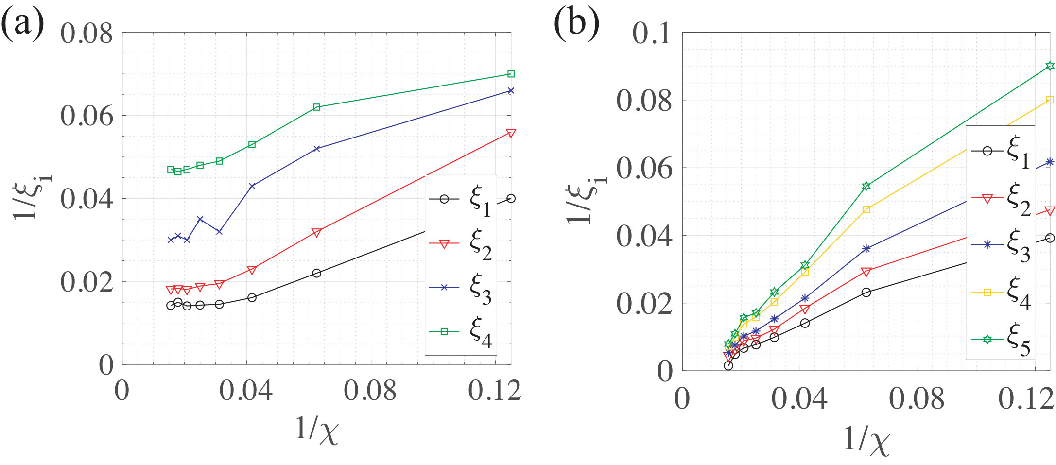 Figure 1
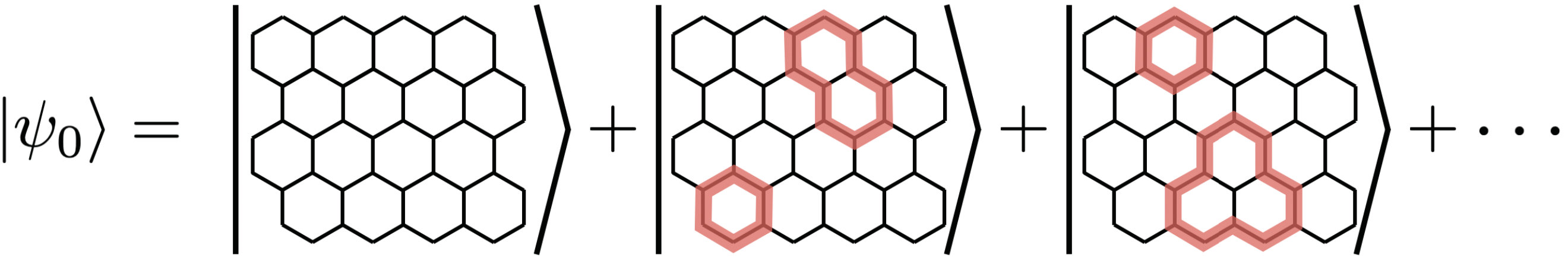 Figure 2
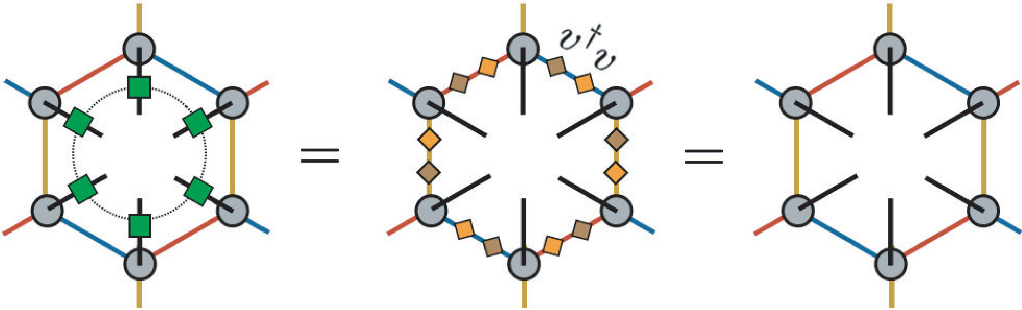 Figure 3
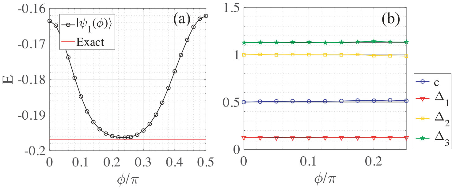 Figure 4
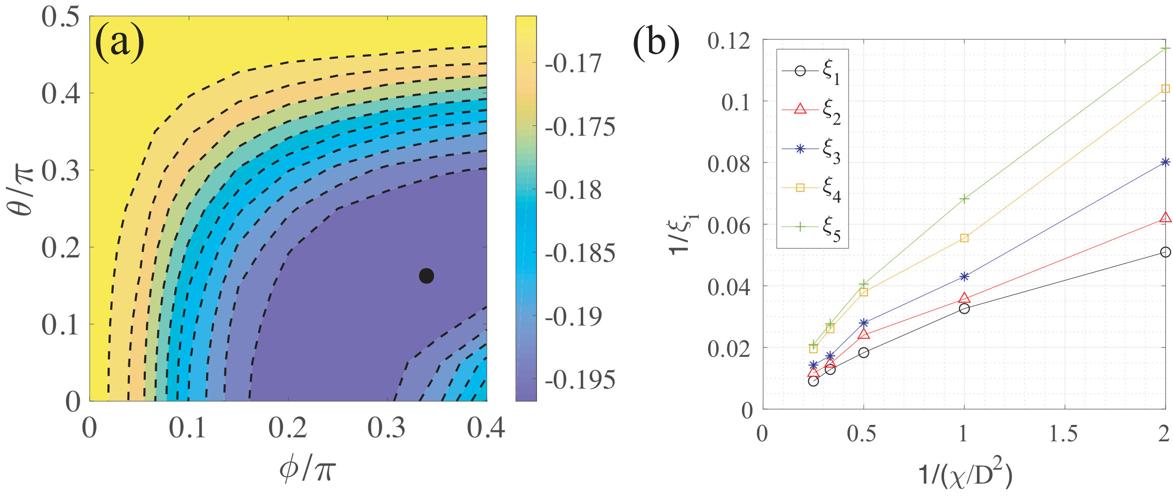 Figure 5
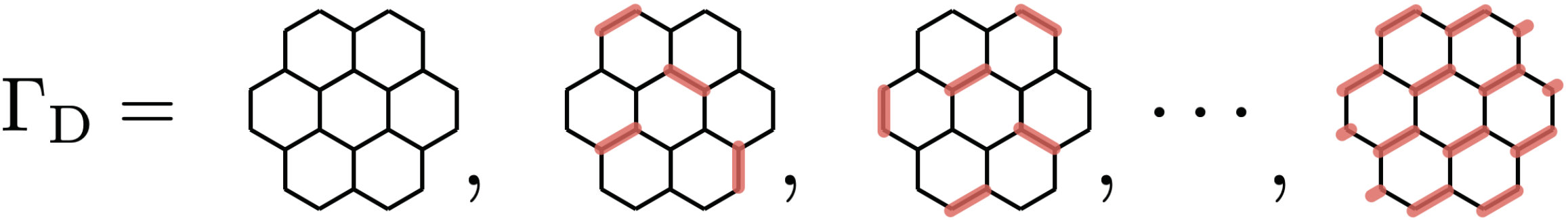 Figure 6
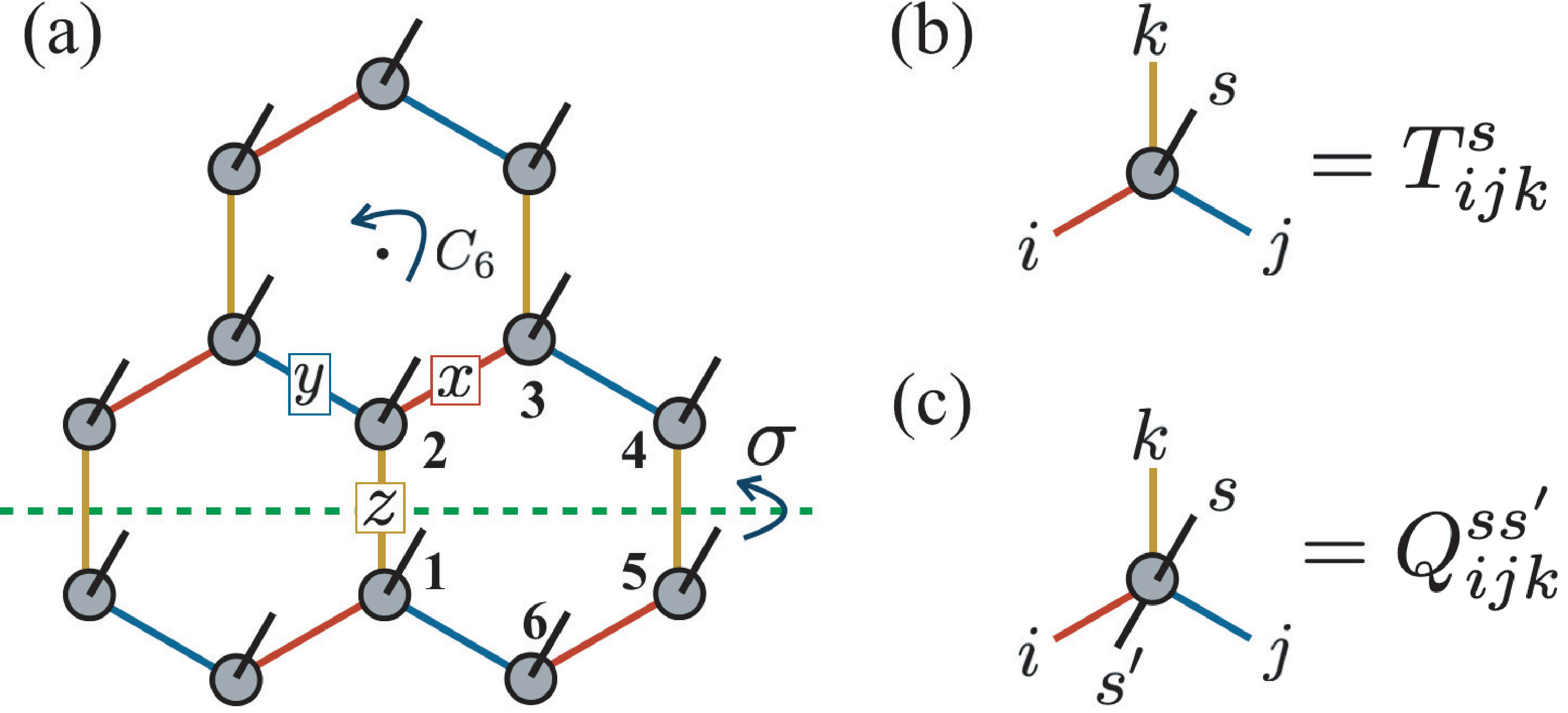 Figure 7
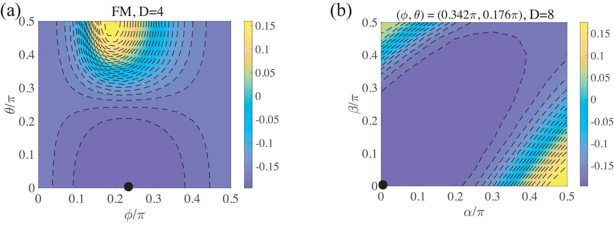 Figure 8
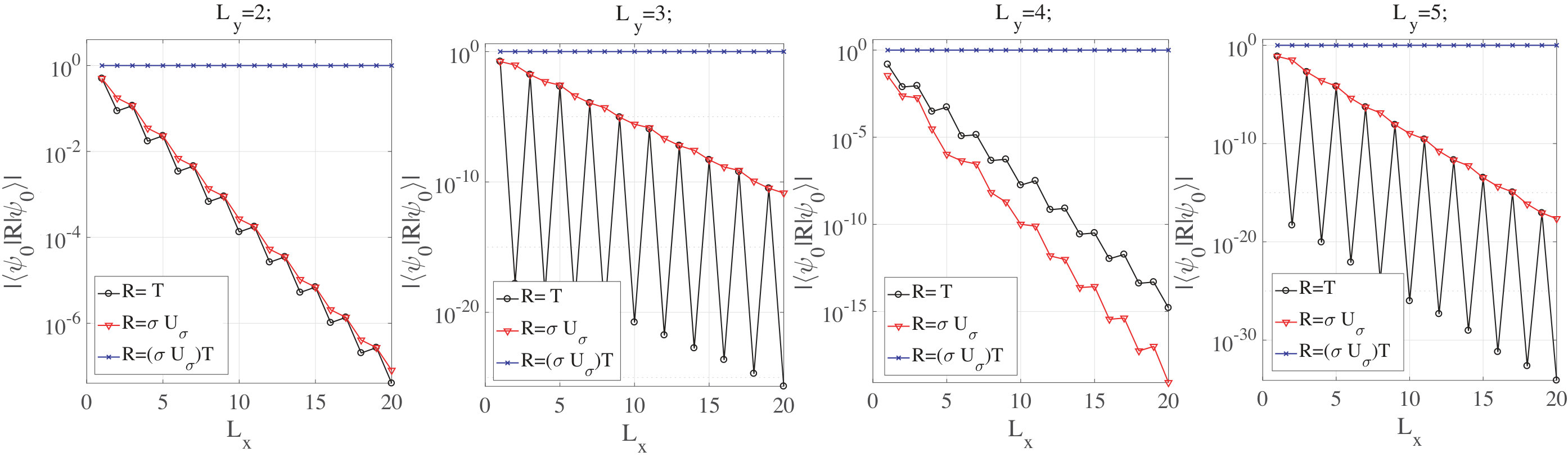 Figure 9
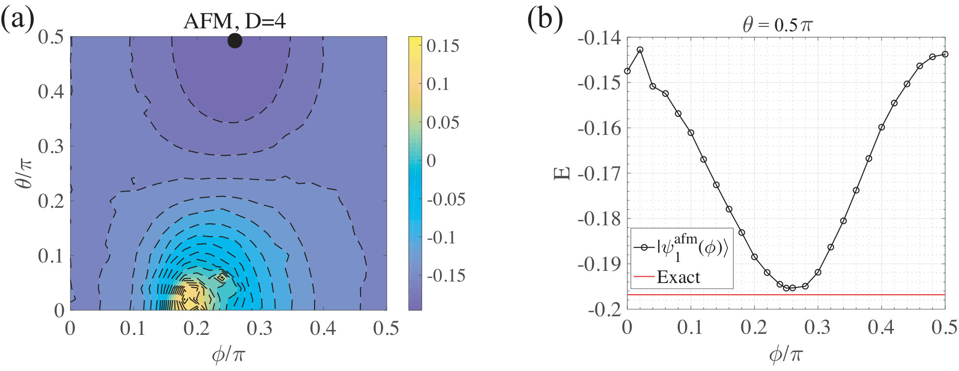 Figure 10
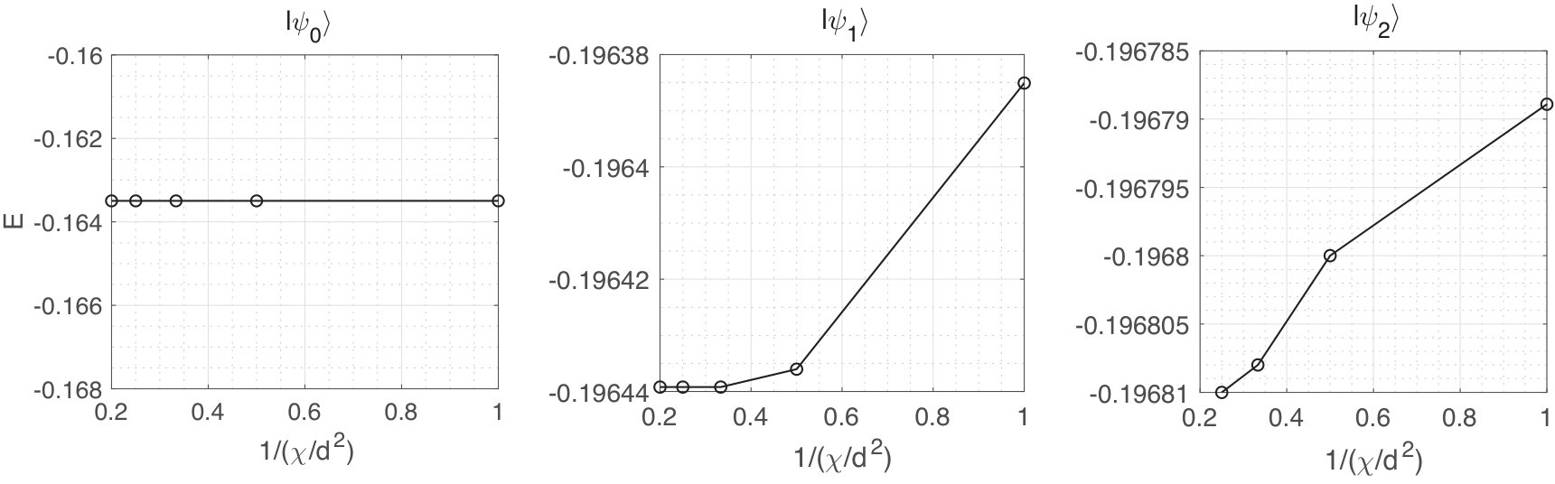 Figure 11
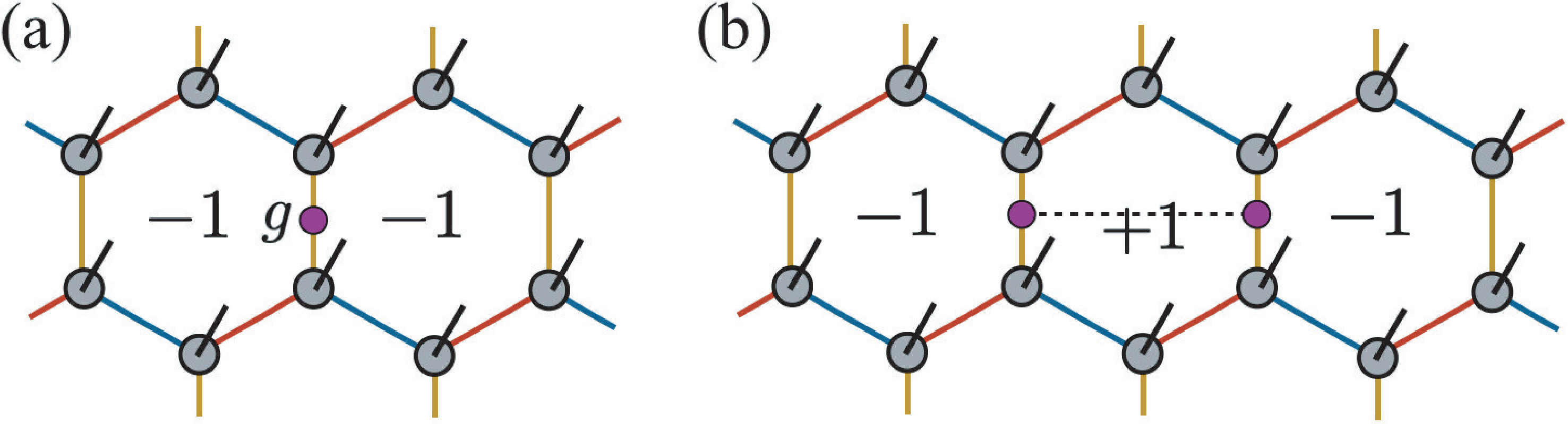 Figure 12
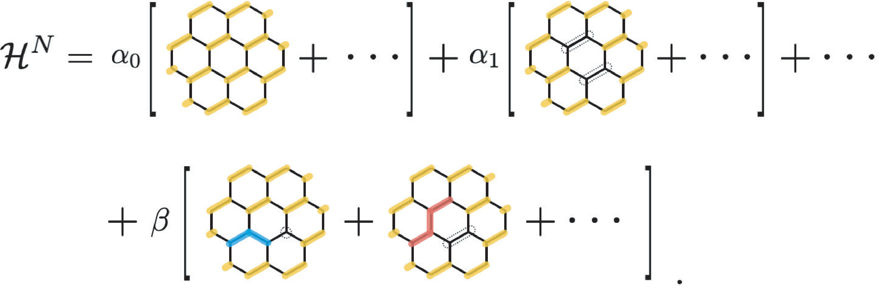 Figure 13
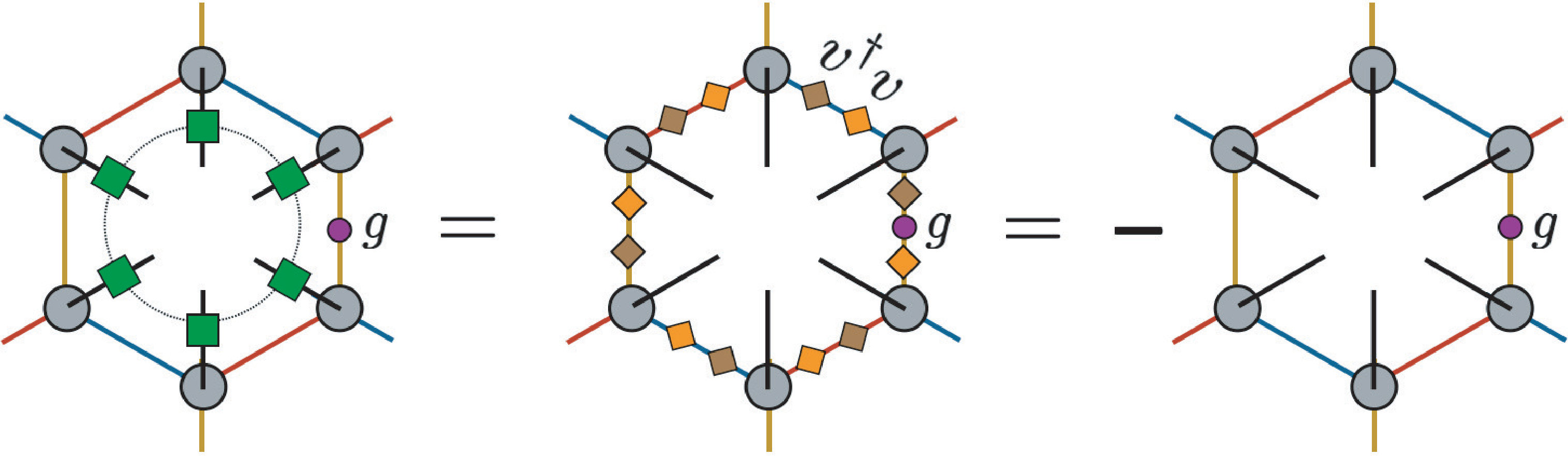 Figure 14
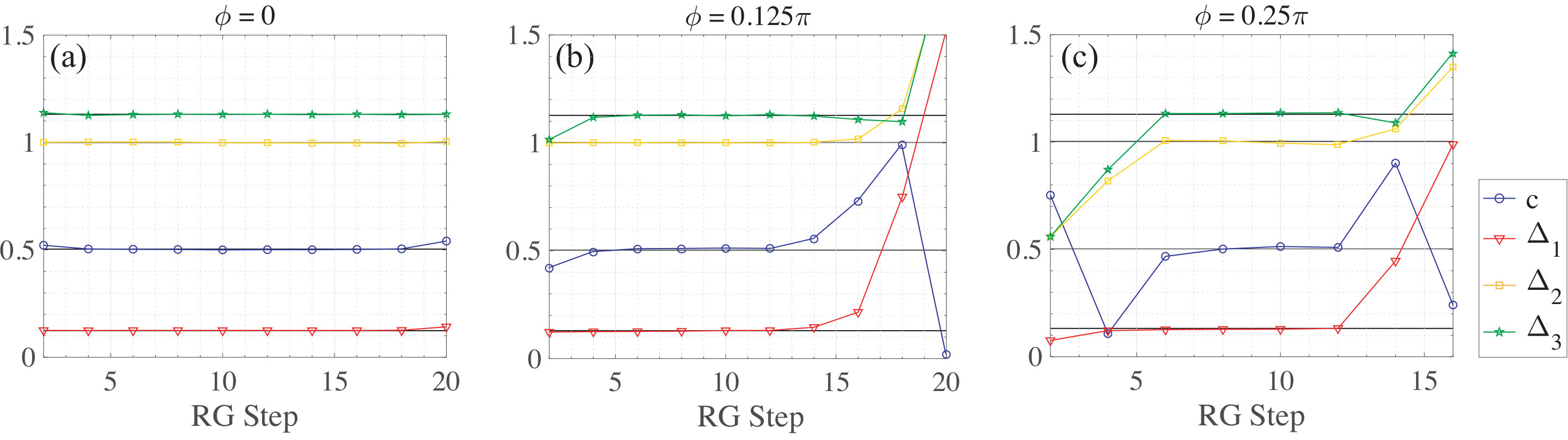 Figure 15
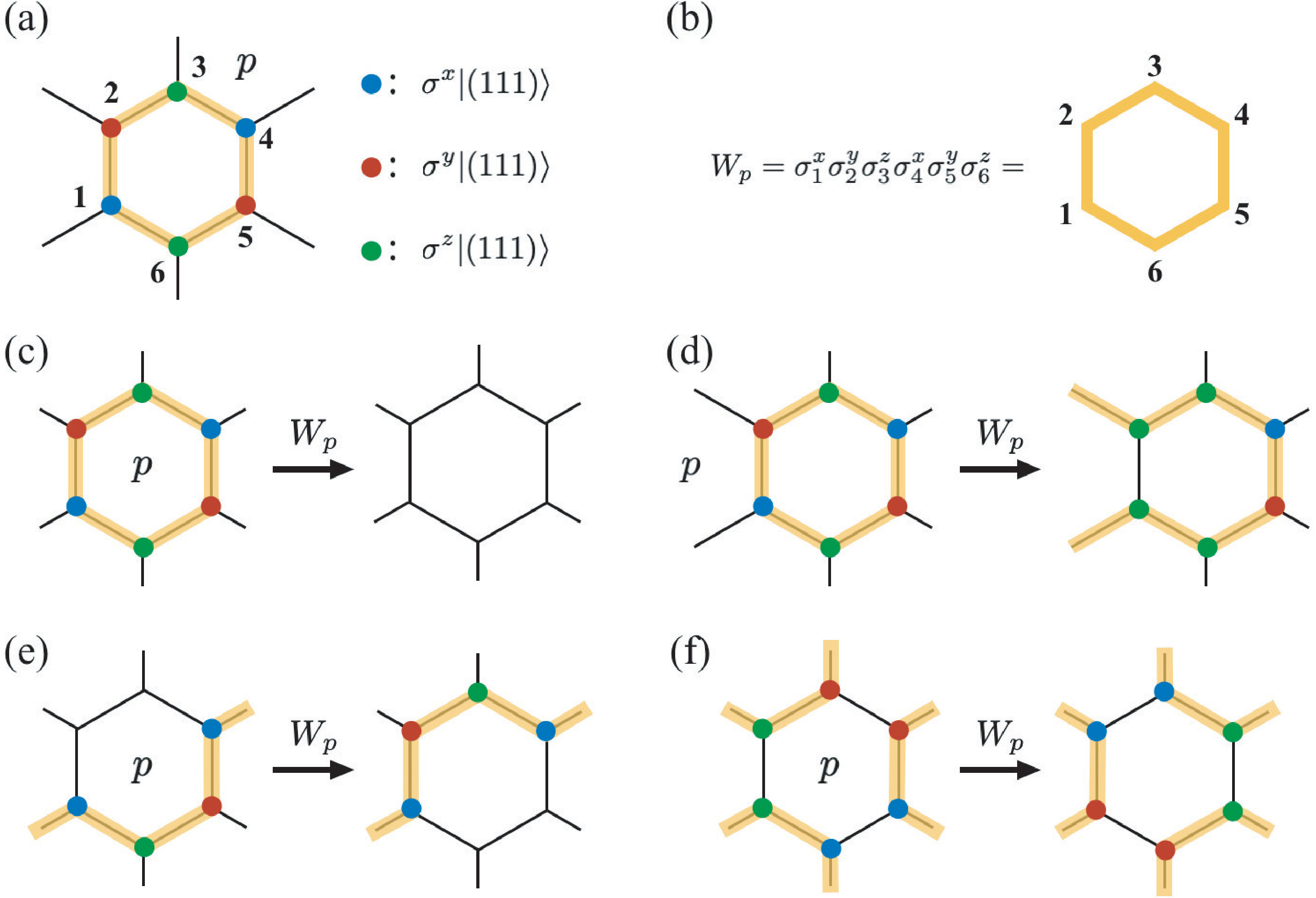 Figure 16
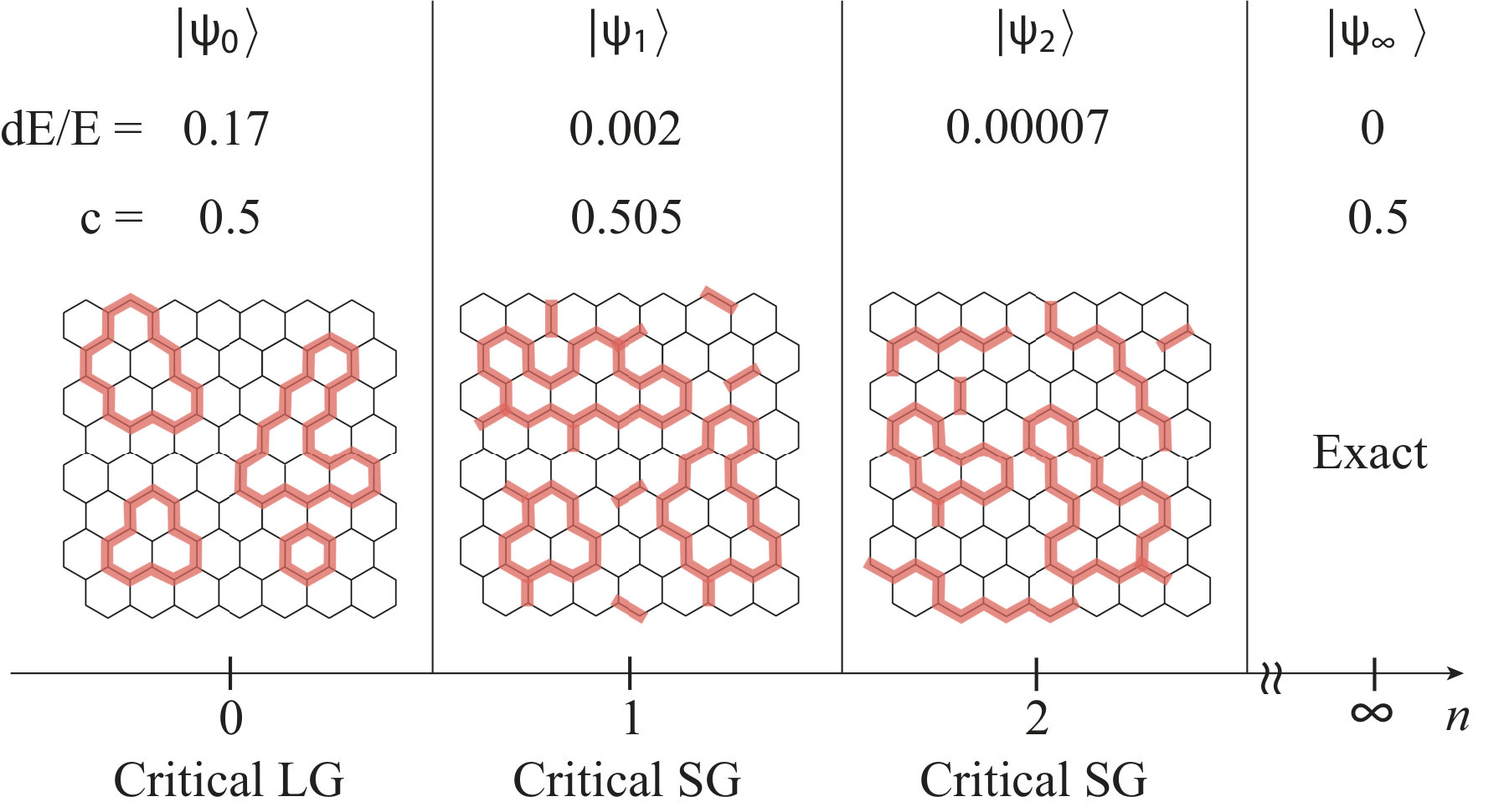 Figure 17
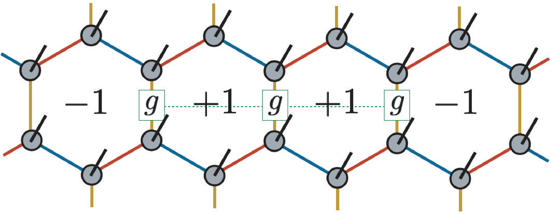 Figure 18
Peer Reviews
No public reviews on file for this paper yet. If you reviewed it on a platform where reviews are public (OpenReview, ICLR, NeurIPS, ICML), you can paste yours below so the community can read it here.
Videos
No videos yet. Explain this paper in a talk, walkthrough, or lecture? Add one.
Gapless Kitaev Spin Liquid to Classical String Gas through Tensor Networks
Hyun-Yong Lee
Institute for Solid State Physics, University of Tokyo, Kashiwa, Chiba 277-8581, Japan
Ryui Kaneko
Institute for Solid State Physics, University of Tokyo, Kashiwa, Chiba 277-8581, Japan
Tsuyoshi Okubo
Department of Physics, University of Tokyo, Tokyo 113-0033, Japan
Naoki Kawashima
Institute for Solid State Physics, University of Tokyo, Kashiwa, Chiba 277-8581, Japan
Abstract
We provide a framework for understanding the gapless Kitaev spin liquid (KSL) in the language of tensor network (TN). Without introducing Majorana fermion, most of the features of the KSL including the symmetries, gauge structure, criticality and vortex-freeness are explained in a compact TN representation. Our construction reveals a hidden string gas structure of the KSL. With only two variational parameters to adjust, we obtain an accurate KSL ansatz with the bond dimension in a compact form, where the energy is about higher than the exact one.
Introduction- Quantum spin liquids (QSL) represent a state of quantum matter which is not characterized by any local order parameters even at zero temperature. These novel states are expected to exhibit long-range entanglement leading to the topological order and fractionalized excitationsSavary and Balents (2017). For example, the nearest-neighbor resonating valence bond (nnRVB) statesAnderson (1987) have been extensively studied as variational wavefunctions for the ground states of frustrated quantum magnetsMoessner and Sondhi (2001); Wen (2002). Indeed, the nnRVB states are topologically orderedMoessner and Sondhi (2001); Wen (2002); Zhou et al. (2017); Poilblanc et al. (2012); Lee et al. (2017) and support spinon excitations carrying the fractionalized quantum numberWen (2002); Zhou et al. (2017). However, since they are not exact ground states of the antiferromagnetic Heisenberg model, variational methods with the nnRVB states have been employed to search for true ground statesKaneko et al. (2014); Jiang et al. (2016); Iqbal et al. (2016); Mei et al. (2017). The Haldane phase, which is also known as a symmetry-protected topological phase, is another fascinating phase one can find in the quantum spin chain. The novel character that discriminates the Haldane phase from trivial gapped states was most clearly revealed by the discovery of Affleck–Kennedy–Lieb–Tasaki (AKLT) model and its exact ground state or AKLT stateAffleck et al. (1987). The compact representation of AKLT stateKlümper et al. (1993) provided a new insight into the Haldane phase. In addition, it was subsequently used in a variety of contexts for variational calculations on the quantum spin systemsKlümper et al. (1993); Kolezhuk and Mikeska (1998).
Kitaev honeycomb model (KHM) is an exactly soluble model which exhibits gapless and gapped KSL ground states with fractionalized excitationsKitaev (2006). Recent successful realizations of Kitaev materialsKhaliullin (2005); Jackeli and Khaliullin (2009); Plumb et al. (2014); Zhou et al. (2016); Banerjee et al. (2016); Trebst (2017); Singh and Gegenwart (2010) triggered a burst of theoretical investigations on KHM and its extensionsKimchi and You (2011); Catuneanu et al. (2018); Gohlke et al. (2018). In addition, due to the non-Abelian phase of the KSL driven by the magnetic fieldJiang et al. (2011); Zhu et al. (2018) and its potential application to quantum computation, it has been a subject of active research for the last decade. We refer the readers to Ref.Nayak et al. (2008) for an exhaustive list of relevant literature. The TN methods have been also employed to represent the KSLSchmoll and Orús (2017); Osorio Iregui et al. (2014). However, the Majorana basis TN requires a three-dimensional structure which makes it impractical as a tool for the numerical optimizationSchmoll and Orús (2017). On the other hand, the spin basis TN study, which was done with the computationally expensive optimization, suffers from undesirable breaking of symmetriesOsorio Iregui et al. (2014). In this Letter, we provide a compact TN representation for KHM that is defined with the spin basis and retains various symmetries.
Model. The KHM is defined asKitaev (2006)
[TABLE]
where stands for a pair on the links connecting sites and as depicted in Fig. 1 (a). As demonstrated in Kitaev’s seminal workKitaev (2006), the Hamiltonian commutes with the so-called flux operators defined on all hexagonal plaquette (): with where the site indices 1-6 are defined in Fig. 1 (a). Therefore, the Hilbert space is sectorized by each flux number . Even further, in each sector, the KHM becomes a noninteracting Majorana fermion hopping model in the background of static gauge fields. The ground states live in the vortex-free sector ( for all ), which form a critical KSL phase around the isotropic point (). In this Letter, we only consider the isotropic point at which the KHM is invariant under the following symmetry transformations: and , where , , and , respectively denote the spatial rotation and inversion as depicted in Fig. 1 (a). One can easily verify . Also, the KHM is invariant under the time-reversal and translational symmetries.
Tensor network representation. We employ the tensor product state (TPS) representation Verstraete et al. (2008). Since the KSL is a zero-flux state You et al. (2012), we reasonably assume the TPS to be translationally symmetric. Additionally, we assume that the tensor does not depend on the sublattice, and therefore our ansatz is rewritten as where tTr stands for the tensor trace or contraction of all virtual indices , labels the site, with being the local quantum number. Its graphical illustration is presented in Fig. 1, where the black open leg denotes the physical degrees of freedom. In what follows, we will construct the local tensor (we identify and and call both “tensor” hereafter) with consideration for the symmetries, the vortex-free condition and gauge structure. In the main text, we only discuss the ferromagnetic model , since the antiferromagnetic one is a trivial generalization and discussed in the supplementary material (SM) Lee et al. (2019).
Zeroth order tensor. We begin with introducing a bond dimension tensor product operator (TPO) referred to as the loop gas (LG) operator, with a building block tensor
[TABLE]
which is depicted in Fig. 1 (c). The virtual indices and range from 0 to 1 (), and non-zero elements of -tensor are and . To simplify the notation, we define a local operator . One can verify in the local tensor level that the LG operator respects the symmetries of KHM. For instance, applying on the -tensor leaves it intactly, i.e.,
[TABLE]
Here, we use the facts that the -transformation rotates the spin, i.e., , while the -rotation permutes the virtual indices as followse . Therefore, the resulting LG operator is invariant under the -transformation, and other symmetries of KHM can be shown in a similar wayLee et al. (2019). Note that the -operator satisfies the following relation
[TABLE]
with a matrix , of which non-zero elements are and , acting on the virtual bonds. Repeated indices are summed over, except where explicitly stated otherwise. Using Eq. (3), one can verify a relation . To be more specific, the invariance of a patch of under the action of can be shown as follows:
[TABLE]
where the connected green squares denote , and a physical leg is omitted for simplicity. Here, Eq. (3) and are used in the first and second equalities, respectively. This remarkable relation guarantees a quantum state , where is an arbitrary state, being vortex-free and thus non-magnetic. Notice that the LG operator is identical to the projector up to a normalization factor.
Regarding the -symmetry, let us apply on a product state , where denotes a spin aligned along (1,1,1) direction: . Note that the ansatz is a classical ground state respecting the -symmetry. Now, we define a quantum state which consists of a building block tensor
[TABLE]
We refer to it as zeroth order tensor. By virtue of the -tensor in , one can visualize the ansatz as follows
[TABLE]
Here, the empty site stands for state while the red loops denote the product of and states depending on the direction of loop on each site.
By computing the norm of the LG ansatz, we can show its criticality. To this end, we first note that the LG operator is hermitian as well as idempotentLee et al. (2019): where is a total number of the loop configuration in the system. Using such properties and a simple identity , it is straightforward to show that the norm of reads
[TABLE]
where denotes a set of all possible loop configurations and is a total length of loops in a configuration . Also, stands for the partition function of the classical loop gas model with the fugacity , which is exactly solvable and critical at Nienhuis (1982). It indicates that the norm of is exactly mapped into the partition function of the critical classical model which guarantees the criticality of Ardonne et al. (2004). In addition, the Ising conformal field theory (CFT) with the central charge is known to characterize the critical LG modelNienhuis (1982), which is consistent with the KSL of KHMMånsson et al. (2013); Lahtinen et al. (2014); Meichanetzidis et al. (2016).
The LG structure encoded in the -tensor is useful in describing the vortex excitation of the KSL. To see this, we first note that the -tensor is invariant under a gauge transformation , i.e. , and thus
[TABLE]
With a trivial gauge transformation being a two-dimensional identity matrix, they form a invariant gauge group (IGG). String-like action of on links would twist the gauge fieldsKitaev (2006) along the string and hence create two vortices at both ends as demonstrated below:
[TABLE]
where in the hexagon denotes . One can explicitly showLee et al. (2019) such creation and move of fluxes using Eq. (3).
Finally, we measure the KHM energy (per bond) of and obtain which is rather higher than the exact one Kitaev (2006). Details in numerics will be discussed later. By construction, the LG ansatz made of zeroth order tensor satisfies most of the physical constraints respected in the KSL [see SM for the time-reversal and symmetries] but is energetically far away from the exact solution. In what follows, we present a simple but effective TPO () applied to the LG ansatz which reduces the energy greatly without violating the constraints. We refer to it as the dimer gas (DG) operator.
Higher order tensors. The DG operator is defined by with
[TABLE]
Here, non-zero elements of -tensor are and with , and is a real(or pure imaginary) variational parameter fixing the fugacity of a dimer. In this context, the dimer denotes the operator . Then, the DG operator can be interpreted as a sum of all possible dimer configurations, i.e., where is defined for each dimer configuration , and is the set of all dimer configurations:
[TABLE]
Due to , it is obvious that commutes with for any , and hence does; . In fact, we can easily prove and that the DG operator respects all symmetries of the KSL Lee et al. (2019). Therefore, its multiplication to does not contaminate the features of the KSL regardless of . Moreover, it can be expressed as the polynomial function of the KHM Hamiltonian, which may be the reason why it improves the energy of the ansatz quite efficiently. The first key observation is that we can graphically represent Eq. (1) raised to the -th power as the linear combination of elements of as
Here, the number of sites in the system is assumed to be . The terms grouped with a coefficient are the fully-packed configurations while the second ones are configuration with dimers. The terms on the second line have -mers longer than dimer, e.g. trimer . All those terms with -mers are canceled by the anticommutativity of Pauli matrices, and thus . Note that the configurations with the same number of dimers share the coefficient which resembles the . Then, one can recast it as with proper coefficients . Note that our approach is not a perturbative oneVanderstraeten et al. (2017).
Now, we define the -th order ansatz as having complex variational parameters. Due to the application of the DG operator, the ansatz can be interpreted as a string gas state which is a linear superposition of string configurations. The string configuration consists of open and closed strings, connected loops and string-connected loops as depicted in Fig. 2. The building block tensor of , referred to as the -th order tensor, is obtained by applying the -operator -times on the zeroth order tensor in Eq. (14). The bond dimension scales as . Note that the LG feature or -tensor in the zeroth tensor is inherited by all higher order tensors. Furthermore, the -operator is invariant only under the trivial gauge transformation, and thus its action does not enlarge the IGG of which the non-trivial element is simply . In contrast to the zeroth order case, the norm of does not map to the LG model. However, by employing the loop TN renormalizationYang et al. (2017), we numerically prove that the -th order ansatz are also critical and characterized by the Ising CFT as summarized in Fig. 2. We also present the best variational energies at each order in Fig. 2, and the details are given below.
Variational ansatz. Now, we turn on and tune variational parameters to obtain a better ansatz than the zeroth one. We parametrize the -tensor as follows: , , and hence . For measuring the energy, we employ the corner transfer matrix renormalization group method (CTMRG)Nishino and Okunishi (1996); Orús and Vidal (2009); Corboz et al. (2010) of which accuracy is controlled by the dimension of CTM. The parallel C++ library mptensorMorita et al. (2016–) is utilized to perform CTMRG.
Let us begin with the first order ansatz and its building block tensor
[TABLE]
where and . The energy of is presented in Fig. 3 (a) as a function of , of which the lowest is found at . Here, we fix . It is remarkable that the first order tensor () already attains such a small error of . Furthermore, we perform the loop TN renormalization to evaluate the norm of and extract the central charge and scaling dimensions presented in Fig. 3 (b)[see SM for more details]. All those are in excellent agreement with the ones of Ising CFT, and therefore our ansatze are critical and belong to the same universality class.
To obtain an ansatz even closer to the KSL, we consider the second order ansatz and tensor ():
[TABLE]
Its overall energy landscape is shown in Fig. 4 (a) as functions of and minimized at . After an additional scaling with respect to Lee et al. (2019), we obtain the best variational ansatz with which is only higher than the exact one. Also, using the environment tensorsLee and Kawashima (2018), the five largest correlation lengths () are extracted and shown in Fig. 4 (b), which are diverging with . Analogous figure is shown for in SM. Therefore, we reasonably conclude that the ansatz made of higher order tensors form a family of gapless states which we believe are smoothly connected to the exact KSL and, as a series, converge to it.
Further, we foundLee et al. (2019) that applying the (111)-direction magnetic field drives the ansatze into the gapped phaseKitaev (2006). We speculate that these gapped ansatze host non-Abelian anyonic excitations. The description of the non-Abelian and Abelian topological phases under the LG and SG schemes is an interesting question, and now further study is in progressLee et al. .
Conclusion. Based on the physical and gauge symmetries and the vortex-free condition, we have constructed the compact TN representation, which generates a family of KSL-like states sharing the features of the KHM ground state. In this sense, the ansatze given in this study are analogous to the AKLT state as a member of the Haldane states or the RVB state as an ansatz of frustrated quantum magnetsAffleck et al. (1987); Wen (2002). Under this scheme, the string gas structure of the KSL comes in sight clearly which offers a novel viewpoint for the KSL and its physics. It also provides an intuitive picture for the KSL in the spin language without referring to the Majorana fermion, which has never been provided before. There are many generalizations that one can envision as well as concrete open questions involving the LG and SG ansatze, e.g., general LGs having larger internal degrees of freedom and their parent Hamiltonians. The relation between the general LGs and the string-net statesFendley (2008) is another interesting question to ask. We also find that the ansatz discussed in the present Letter provides a good initial state for variational method for the KHM with the magnetic fieldKaneko et al. . Further, for the anisotropic KHM, one can choose the initial magnetic state which differs from the state and introduce a bond-dependent dimer fugacity as additional variational parameters to optimize the modelLee et al. . Therefore, we expect our work could furnish a better understanding of KSL and its neighboring phases observed in the Kitaev quantum magnets such as -RuCl3 Banerjee et al. (2016, 2018) and studied theoretically in extended KHMsJackeli and Khaliullin (2009); Chaloupka et al. (2010); Singh and Gegenwart (2010); Kimchi and You (2011); Gohlke et al. (2018). Using two variational parameters, the accuracy of in energy is obtained, which has never been achieved by other numerical optimizationsPhien et al. (2015); Corboz (2016); Vanderstraeten et al. (2016). This high accuracy, together with the observed systematic convergence, leads us to believe that the present scheme not only correctly captures the essence of KSL physics, but also provides a new direction for quantitatively accurate description of quantum spin liquids.
Acknowledgements.
Acknowledgements- The computation in the present work was executed on computers at the Supercomputer Center, ISSP, University of Tokyo, and also on K-computer (project-ID: hp180225). N.K.’s work is funded by ImPACT Program of Council for Science, Technology and Innovation (Cabinet Office, Government of Japan). H.-Y.L. was supported by MEXT as “Exploratory Challenge on Post-K computer” (Frontiers of Basic Science: Challenging the Limits). R.K. and T.O. were supported by MEXT as “Priority Issue on Post-K computer” (Creation of New Functional Devices and High-Performance Materials to Support Next-Generation Industries), and JSPS KAKENHI No. 15K17701, respectively.
I Symmetries of the Loop Gas Operator
In the main text, we define the loop gas (LG) operator with the building block tensor
[TABLE]
where , and the non-zero elements of -tensor are
[TABLE]
We consider unitary operators
[TABLE]
which transform the Pauli matrices in the following way:
[TABLE]
Let us see how the LG operator transforms locally under the and rotations:
[TABLE]
where Eq. (4) is used. Now, we consider the spatial rotation and reflection transformations defined in Fig. (1) in the main text. Such lattice symmetry transformations permute the virtual indices: and . Let us apply those transformations on Eq. (5),
[TABLE]
where we use the fact that the -tensor is fully symmetric under any permutation. The first equation in Eq. (6) directly indicates that the operator , and thus the LG operator, is invariant under the -transformation, . Note that the length of any loop on the honeycomb lattice is even, which indicates that the extra minus signs in the second equation in Eq. (6) are redundant. Therefore, the LG operator remains invariant under the -transformation: . Now, we consider the time-reversal transformation which transforms the operator as follows:
[TABLE]
where is used. Even though the -tensor is not symmetric under the time-reversal transformation, an additional gauge transformation can restore its original form, i.e.,
[TABLE]
Therefore, the LG operator is time-reversal symmetric: . By construction, the translational symmetry is respected in the LG operator, and therefore it keeps all symmetries of the isotropic Kitaev honeycomb model.
II Details on the Dimer gas operator
As demonstrated in the main text, in order to reduce the energy, we define the DG operator with
[TABLE]
and , and the non-zero elements of -tensor are
[TABLE]
The constant is a variational parameter. As shown in the previous section, let us first consider the -symmetry, i.e., :
[TABLE]
where we used the fact that the -tensor is invariant under any permutation in the indices. Above relation implies . Next, under the -symmetry, the transforms as
[TABLE]
Here, although an extra minus sign appears, it will be canceled after after contraction since the dimer is a two-site object. Consequently, the DG operator is symmetric under the -transformation: . As for the time-reversal symmetry, one can show
[TABLE]
Therefore, in any case, the DG operator is invariant under the time-reversal transformation: . Consequently, if one can apply the PEPO on some ansatz respecting the symmetries, then the resulting state is also guaranteed to satisfy those symmetries.
III The time-reversal symmetry and -symmetry of ansatze
The zeroth order ansatz is obtained by contracting the zeroth order tensor
[TABLE]
Let us see how it transforms under the -symmetry and time-reversal symmetry ,
[TABLE]
where denotes a spin aligned along direction: . Here, relations , and are used. Note that one cannot restore and to by applying a gauge transformation. Consequently, the zeroth order tensor does not ensure the resulting state to be time-reversal symmetric and -symmetric. However, it is invariant under the combination of and transformations, i.e., . More precisely, the zeroth order tensor is transformed as follows
[TABLE]
where Eqs. (6) and (7) are used. The overall phase does not affect the resulting state, and therefore the zeroth order ansatz is invariant under the -transformation.
Even though the building block tensor does not guarantee the and symmetries, those symmetries might be restored in a larger unit-cell. In order to carve this out, we measure the fidelity between the states and its transformed one on a torus geometry with size , where and , and denotes the number of unit-cell on horizontal and vertical directions. The results are shown in Fig. 1. As one can see, the transformed state becomes orthogonal to each other, and thus not symmetric under the transformations. Then, how can we make them symmetric? In fact, Eq. (15) provides a quick cure to construct an ansatz respecting both the and symmetries by doubling the bond dimension:
[TABLE]
where and
[TABLE]
The resulting state from above tensor is simply and thus, by construction, invariant under the time-reversal operation. The symmetry is also guaranteed as shown below
[TABLE]
which is restored to its original form by flipping in with a proper coefficient to eliminate the minus sign in the second line. It can be simply done by applying a gauge trasformaion
[TABLE]
such that
[TABLE]
This procedure also applies to the higher order tensors, and therefore one can always construct a higher order ansatz, which is time-reversal and -symmetric, by doubling the bond dimension.
IV Manipulation of vortices
As mentioned in the main text, one can create the vortices by acting the non-trivial elements of invariant guage group (IGG) on the virtual bonds. Let us see how it happens. For simplicity, we only consider the zeroth order tensor with , but its generalization to the general case is straightforward. In the main text, we explicitly showed that a plaquette patch of the LG operator is invariant under the action of flux operator using Eq. (3) in the main text. Let us consider the same tensor network except that the is inserted between two sites as depicted below:
[TABLE]
where the connected green squares denote the flux operator while
[TABLE]
In the last equality, we use and . Therefore, the resulting state is an eigenstate of the flux operator with the eigenvalue . The vortex is created. Similarly, another vortex is created on the opposite plaquette covering the -inserted bond as depicted in Fig. 2 (a). Inserting another in the plaquette, the minus sign will be canceled such that the vortex is removed. But, on the opposite plaqutte of newly -inserted bond, another vortex is created. In other words, the vortex can be moved from a plaquette to another one as demonstrated in Fig. 2 (b). The -tensor embedded in the DG operator is invariant only under the trivial gauge transformation , and thus the IGG of the DG operator is the trivial IGG. It indicates that the multiplication of the DG operator does not enlarge the IGG. Therefore, one can create and move the vortices with with the higher order tensors and ansatze.
V Loop Configurations
V.1 Deformation of loops
As mentioned in the main text, the zeroth ansatz has the quantum loop gas structure. In other words, the ansatz are represented by linear superpositions of all possible closed loop configurations with an equal weight. Here, the loop denotes the product of and states along the loop as depicted in Fig. 3 (a), while an empty state is simply . By applying the flux operator , one can deform the loop configurations following a simple rule. First, one regards the flux operator on as a loop along the boundary of as demonstrated in Fig. 3 (b). Then, we put on a loop gas configuration and draw the loop along the plaquette. If some part of loops are overlapped, then we eliminate the overlapped fragments. This procedure does not break any loop but just deform or detour the loops. Also, it does not give any extra phase after the deformation. For example, applying the flux operator on in Fig. 3 (a), then the and apply on and , respectively. Therefore, the local states on the sites and rotates as follows:
[TABLE]
The phases are canceled each other, and a part of loop on the bond between the sites 3 and 4 is deleted and extended to wrap the plaquette . In Fig. 3 (c)-(f), we present some exemplary deformations of some loops by applying the flux operator. Using these local deformations, one can completely remove some loop configurations by applying the flux operators or create them from empty configurations.
V.2 Norm of
The norm of wavefunction contains important informations on the low-lying excitations in the system. In this subsection, we compute the norm of state. It is easy to see that an inner product between the loop free and an arbitrary loop configurations is simply
[TABLE]
where and denote respectively the arbitrary loop configuration and loop free configuration and is the total length of loops in the configuration . Here, we used . As explained in the previous subsection, any loop configuration can be obtained by a product of flux operators, i.e.,
[TABLE]
where denotes a proper choice of plaquettes to create the from the loop free configuration. Then, the norm of is rewritten as
[TABLE]
We use the fact that in the third equality, and Eq. (24) is substituted in the last equality. The norm of turns out to be the partition function of the loop gas model at a critical point as presented in the main text.
V.3 Norm of
The norm of does not map to the exactly solvable point of the loop gas model. Therefore, we employ the loop tensor network renormalization (LTNR) to numerically obtain the norm of and extract the central charge and scaling dimensions . Results for and are shown in Fig. 4 as a function of the real space renormalization step (RG step). Here, the bond dimension of LTNR is fixed to . The number of iteration for loop optimization varies up to 20 to find the best ansatz at each RG step. As shown in Fig. 4 (a), at where the tensor becomes zeroth order one, the conformal data match nicely with the exact values from Ising universality class and shows a stable behavior up to about 20 RG step. Although the accuracy of LTNR becomes less as increasing the fugacity of dimer operator , we could obtain reasonable and consistent results up to around as presented in Fig. 4 (b) and (c).
VI General dimer fugacity and energy land scapes
Generally, the variational parameter in the DG operator is allowed to be complex though it breaks the time-reversal symmetry. The results with only real parameters are shown in the main text. Here, the energy dependence on the complex coefficients is presented and briefly discussed. The first order ansatz is in general defined as
[TABLE]
where the -tensor in the tensor is parameterized as follows: and . Here, the parameter is additionally introduced to give an arbitrary phase. Now, we should fix two parameters to find the energy minimum point, and the energy landscape is shown in Fig. 5 (a). The lowest energy is obtained at . Though we could not mathematically prove whether or not the lowest energy is found by real coefficients, we observe that real coefficients give the lowest energy at several parameter points. Now, let us consider the second order ansatz
[TABLE]
Two phase variables and are introduced. Therefore, we have to fix four independent parameters. Therefore, we present, in Fig. 5 (b), the and dependence of energy only at at which the lowest energy is measured.
VII Antiferromagnetic Kitaev Honeycomb Model
In the main text, we construct the ansatze for the ferromagnetic Kitaev model by applying the LG and DG operators on the classical ground state, where runs over all sites. Following the same strategy, we prepare the classical ground state of the antiferromagnetic model:
[TABLE]
where labels the unit-cell, and denote two different sublattices, respectively. Then, we apply the LG and DG operators on the state as we did in the ferromagnetic model and fix the variational parameters in the DG operator to find the lowest energy ansatz. The zeroth order ansatz gives the energy which is rather higher than the one obtained by the zeroth ansatz of the ferromagnetic model (see the main text). Now, let us see how the DG operator reduces the energy. Here, we only consider the first order ansatz
[TABLE]
where the -tensor in the tensor is parameterized as follows: and . The energy as functions of and is shown in Fig. 6 (a). In contrast to the ferromagnetic case, the lowest energy is found with a negative dimer fugacity or . In Fig. 6 (b), the energy is presented as a function of with . Here, the lowest energy is obtained at , and it is only higher than the exact one. Again, this energy is slightly higher than the one obtained for the ferromagnetic model but still surprisingly close to the exact one with only . We also confirmed that our ansatz for the antiferromagnetic model exhibit critical behavior. We believe that one could obtain much better ansatz by applying another DG operator () as shown in the main text.
VIII Effect of the (111)-direction magnetic field
In the current representation of the KSL, it is naturally anticipated that the (111)-direction magnetic field opens the excitation gap and drives the KSL into the non-Abelian phaseKitaev (2006). Applying the field, the vortex-free condition is not required anymore, and therefore introducing a parameter into the -tensor in is allowedLee et al. (2019), such that and . It is obvious that element generates the local magnetic state while the others do . In the weak-field limit, one can control to modify the weight of LG and reasonably choose , since the (111)-field prefers the state rather than states. Then, the norm of wavefunction maps to [Eq. (6) in the main text], where the model enters into a massive phaseDomb (2000). Consequently, the gap is opened by the magnetic field.
In order to find a better ansatz with , we introduce two additional parameters in , which tune the weight of local states. To be more specific, let us explicitly write down the non-zero elements of the first order tensor where . For simplicity, we redefine the first order tensor as with
[TABLE]
Note that the -tensor is the same as the zeroth order tensor. Now, we assign parameters tuning the weight of states in the -tensor and -tensor, respectively. In other words, the ansatz becomes dependent on three parameters: where the parameter multiplied to the states. For example, the non-zero elements of -tensor are
[TABLE]
Note that the -symmetry is still valid even in the presence of the (111)-field. Therefore, one allows to introduce only a single parameter in the -tensor. Since the -field prefers the local state rather than , one may naively expect that reducing the parameters from 1 helps lowering the energy. Indeed, we found that the energy is optimized at with the energy which is competitive to the one obtained by the numerical optimization Kaneko et al. . The norm of the ansatz is not mapped into the LG model similar to . Therefore, in order to show its gapped nature, we directly measure the most dominant correlation lengths of the ansatz using the environment tensor in CTMRGTakahashi (2005); Lee and Kawashima (2018). The result for ansatz with is presented in Fig. 7 (a) as a function of . As one can see, the correlation lengths converge to finite values with increasing indicating a finite gap in the ansatz. For comparison, those in the critical state are shown in Fig. 7 (b), which exhibit diverging behavior with . Therefore, the gapped ansatz in the presence of (111)-field can be reasonably obtained by giving some fugacity to the tensor element generating state. In addition, it has been recently shownFendley (2008) that the gapped LG having non-trivial inner products between two configurations can be systematically mapped into string-net states describing non-Abelian anyonic excitationsFendley (2008). It strongly suggests that our ansatz belongs to a non-Abelian phase in the presence of (111)-field, which is consistent with the perturbation calculation using the Majorana fermion in Kitaev’s original work Kitaev (2006).
IX -scaling of the variational energies
We provide the bond dimension of CTMRG, , dependence of the variational ansatze shown in the main manuscript. In Figure 8, the scaling behavior of the variational energies of the LG state , the first order SG ansatz , and the second order SG ansatz are shown from left to right, respectively.
The reference list from the paper itself. Each links out to its DOI / PubMed record.
- 1Savary and Balents (2017) Lucile Savary and Leon Balents, “Quantum spin liquids: a review,” Reports on Progress in Physics 80 , 016502 (2017) .
- 2Anderson (1987) PW Anderson, “The resonating valence bond state in la 2cuo 4 and superconductivity.” Science (New York, NY) 235 , 1196 (1987).
- 3Moessner and Sondhi (2001) R. Moessner and S. L. Sondhi, “Resonating valence bond phase in the triangular lattice quantum dimer model,” Phys. Rev. Lett. 86 , 1881–1884 (2001) . · doi ↗
- 4Wen (2002) Xiao-Gang Wen, “Quantum orders and symmetric spin liquids,” Phys. Rev. B 65 , 165113 (2002) . · doi ↗
- 5Zhou et al. (2017) Yi Zhou, Kazushi Kanoda, and Tai-Kai Ng, “Quantum spin liquid states,” Reviews of Modern Physics , 025003 (2017) , ar Xiv:1607.03228 . · doi ↗
- 6Poilblanc et al. (2012) Didier Poilblanc, Norbert Schuch, David Pérez-García, and J. Ignacio Cirac, “Topological and entanglement properties of resonating valence bond wave functions,” Phys. Rev. B 86 , 014404 (2012) . · doi ↗
- 7Lee et al. (2017) Hyunyong Lee, Yun-tak Oh, Jung Hoon Han, and Hosho Katsura, “Resonating valence bond states with trimer motifs,” Phys. Rev. B 95 , 060413 (2017) . · doi ↗
- 8Kaneko et al. (2014) Ryui Kaneko, Satoshi Morita, and Masatoshi Imada, “Gapless spin-liquid phase in an extended spin 1/2 triangular heisenberg model,” Journal of the Physical Society of Japan 83 , 093707 (2014) , https://doi.org/10.7566/JPSJ.83.093707 . · doi ↗