Darboux and Calapso transforms of meromorphically isothermic surfaces
Andreas Fuchs

TL;DR
This paper studies how Darboux and Calapso transformations affect certain special isothermic surfaces with meromorphic Hopf differentials, focusing on their behavior near singularities and the continuity of the transformations.
Contribution
It characterizes the limiting behavior of Darboux and Calapso transforms of meromorphically isothermic surfaces near singularities, providing insights into their continuity and geometric properties.
Findings
Transformations yield new isothermic surfaces away from singularities.
Limiting behavior near zeros or poles is explicitly characterized.
Continuity of transformed surfaces around singular points is analyzed.
Abstract
We consider those simply connected isothermic surfaces for which their Hopf differential factorizes into a real function and a meromorphic quadratic differential that has a zero or pole at some point, but is nowhere zero and holomorphic otherwise. Upon restriction to a simply connected patch that does not contain the zero or pole, the Darboux and Calapso transformations yield new isothermic surfaces. We determine the limiting behaviour of these transformed patches as the zero or pole of the meromorphic quadratic differential is approached and investigate whether they are continuous around that point.
Click any figure to enlarge with its caption.
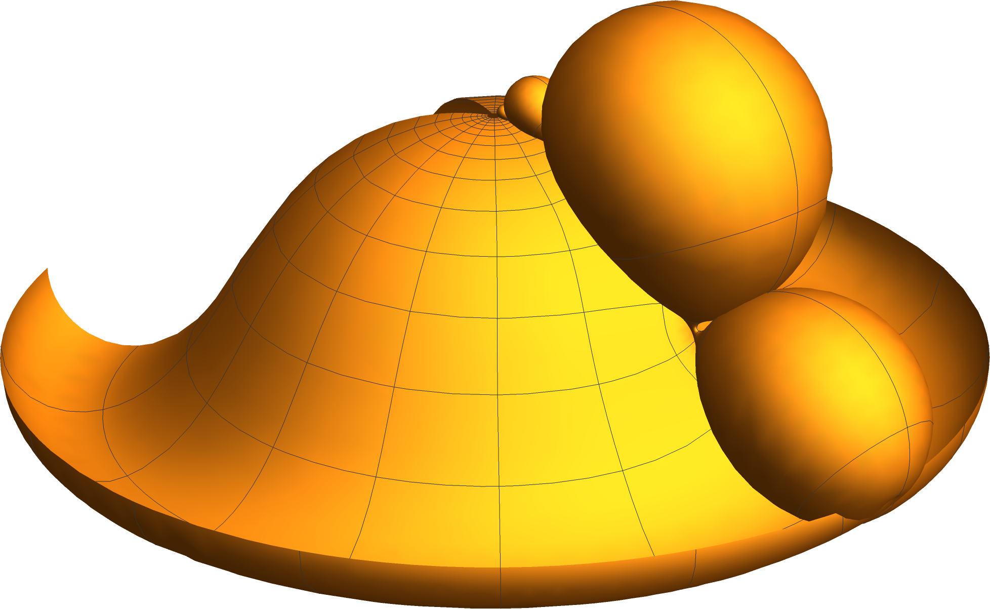 Figure 1
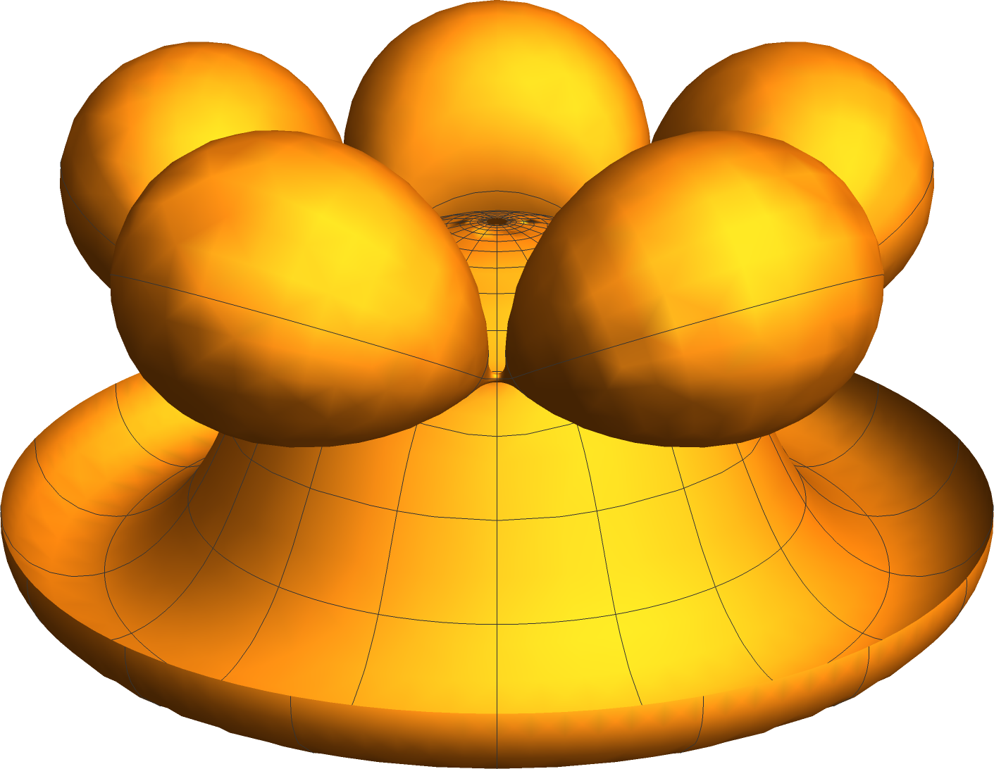 Figure 2
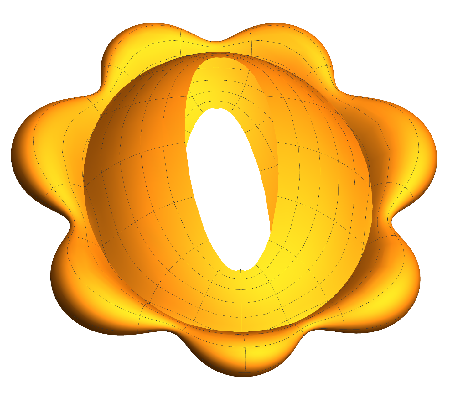 Figure 3
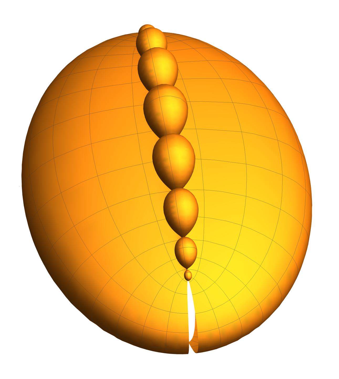 Figure 4
Peer Reviews
No public reviews on file for this paper yet. If you reviewed it on a platform where reviews are public (OpenReview, ICLR, NeurIPS, ICML), you can paste yours below so the community can read it here.
Videos
No videos yet. Explain this paper in a talk, walkthrough, or lecture? Add one.
Taxonomy
TopicsMeromorphic and Entire Functions · Advanced Differential Equations and Dynamical Systems · Holomorphic and Operator Theory
MnSyE120 MnSyE125
Darboux and Calapso transforms of meromorphically isothermic surfaces
Andreas Fuchs
(Jan 17, 2019)
Abstract
We consider those simply connected isothermic surfaces for which their Hopf differential factorizes into a real function and a meromorphic quadratic differential that has a zero or pole at some point, but is nowhere zero and holomorphic otherwise. Upon restriction to a simply connected patch that does not contain the zero or pole, the Darboux and Calapso transformations yield new isothermic surfaces. We determine the limiting behaviour of these transformed patches as the zero or pole of the meromorphic quadratic differential is approached and investigate whether they are continuous around that point.
MSC 2010: 35B40, 51B10, 58K10, 58J72
1 Introduction
In differential geometry transformations of surfaces have contributed considerably in revealing the structures of various surface classes and relations between them. Already in the nineteenth century geometers discovered methods to construct new surfaces from a given one while preserving some geometrical properties, such as the Combescure transformation, which preserves tangent planes up to translations, and the Ribaucour transformation, which preserves curvature lines and an enveloped sphere congruence, see [Bia22] and [Eis62], or [DT03] for a more modern treatment. While these transformations exist for arbitrary smooth surfaces in Euclidean space, others are defined only on subclasses of smooth surfaces, such as the Bäcklund and Lie transformations of pseudospherical surfaces (see [Eis60]) in Euclidean geometry or the Christoffel, Darboux and Calapso transformations of isothermic surfaces in Möbius geometry (see [Bur06, HJ03]) and Lie applicable surfaces in Lie sphere geometry (see [Pem16]). During the last three decades, many of these surfaces have been shown to constitute integrable systems by relating their transformations to a pencil of flat connections, as summarized in [Bur17], cf. [TU00, BC10, Bur06, BFPP93, FP96]. Thereby, their rich transformation theory is placed into common ground and the highly developed tools of integrable systems theory are made available. A discrete version of integrability serves as the guideline for how to define discrete analogues of certain smooth surface classes [BS07].
Transformations of surfaces can also be used to shed a different light on representation formulas. For example, the Weierstrass representation of a minimal surface can be interpreted as the Goursat transform of its Weierstrass data, as explained in [HJ03, HJH17], and Bryant’s representation [Bry87] of CMC-1 surfaces in hyperbolic space can be related to the Darboux transformation of isothermic surfaces, see [HJMN01]. Recently, these and further representation formulas have been linked to the transformation theory of -surfaces in [Pem16].
We are interested in the class of smooth isothermic surfaces, classically characterized by the local existence of conformal curvature line coordinates, away from umbilics. For these surfaces, the transformation theory is defined only locally and away from problematic umbilics. In other words, it is well defined only on the subclass that contains those simply connected isothermic surfaces which can be covered by conformal curvature line coordinate charts. These surfaces, which we call simple isothermic, can equivalently be characterized by the existence of a factorization of the Hopf differential of the surface into a real factor and a nowhere zero holomorphic quadratic differential (cf. [Bur06, HJ03, Smy04]). In particular, a simple isothermic surface cannot contain an umbilic of nonzero index and hence cannot have the topology of the sphere by the Poincaré-Hopf theorem (cf. [Hop89]).
Arguably, this limitation of the transformation theory is not quite satisfactory though as many classical examples of isothermic surfaces are not simple isothermic. For instance, a triaxial ellipsoid, surfaces of revolution which smoothly intersect the axis of revolution, and minimal surfaces with appropriate Weierstrass data all contain umbilics with nonzero index. However, all these examples fall into the class of meromorphically isothermic surfaces, that is, their Hopf differential factorizes into a real factor and a globally defined meromorphic quadratic differential. The globally existing factorization makes this class of surfaces a promising candidate for an extension of the simple isothermic transformation theory.
For a given meromorphically isothermic surface which is not simple isothermic, the transformation theory is still not defined globally. But after removing the zeros and poles of the meromorphic quadratic differential from the domain of the surface and then passing to the universal cover, one obtains a simple isothermic surface as a branched covering of the original surface. One may then ask which transforms of this simple isothermic covering surface descend to surfaces that qualify as transforms of the original meromorphically isothermic surface. More precisely, for a meromorphically isothermic surface with domain , denote by the set of zeros and poles of the meromorphic quadratic differential obtained from the factorization of the Hopf differential. Then the pullback of that surface to the universal cover of is simple isothermic. The fundamental group of acts on the space of transforms of and one question is whether there are transforms which are invariant under this action. These would then qualify as transforms of the original surface restricted to . A second question is how the transforms of behave as one approaches the zeros and poles of . In particular, do the transforms have limits at ?
In this work, we address these questions for the Darboux and Calapso transforms of a simply connected meromorphically isothermic surface where the meromorphic quadratic differential has a pole of first or second order at an interior point , but is nowhere zero and holomorphic otherwise. According to the local Carathéodory conjecture [GK08], these are the only poles that can occur on an isothermic surface. We investigate for which parameters the Darboux and Calapso transforms of the pullback of that surface to the universal cover of are invariant under the action of the fundamental group and what their limiting behaviour at is. We also briefly treat the case where has a zero and argue that it is conceptually much simpler than a pole of . Our results about the limits of transforms at a pole of are generalizations of the corresponding results for transforms of polarized curves, found in [Fuc18b], to surfaces. The action of the fundamental group on the space of Darboux and Calapso transforms however is a novel feature, which is specific to surfaces.
In Sect 2, we present a hierarchy of definitions of isothermic surfaces in the conformal -dimensional sphere , including meromorphically isothermic and simple isothermic surfaces. We then introduce our formulation of the Darboux and Calapso transformations of simple isothermic surfaces using the concept of primitives of the pencil of flat connections associated to a simple isothermic surface. These primitives are Möb-valued maps characterized by
[TABLE]
for any point in the domain. A -Darboux transform of is obtained by acting with on a point and a -Calapso transform is the product of with .
These constructions of the Darboux and Calapso transformations cannot be extended to meromorphically isothermic surfaces. The family of flat connections exists only away from the poles of the meromorphic quadratic differential and, in general, they have nonzero monodromy around poles. Therefore, their primitives do not exist globally, not even away from the poles of . But the primitives along closed loops generate the monodromy group. In Prop 2.5, we use this to derive actions of the fundamental group of a meromorphically isothermic surface with removed poles on the spaces of Darboux and Calapso transforms of its simple isothermic covering. We conclude this section with some results about the case of a meromorphically quadratic differential with a zero.
In Sect 3, we develop tools to analyse the limiting behaviour of the primitives and the monodromy of the flat connections associated to a meromorphically isothermic surface. In particular, we introduce a class of singular flat connections which have a pole at some point in the domain. We then analyse the limiting behaviour of primitives of such connections at the pole and investigate the structure of their monodromy.
In Sect 4, we consider the case of a simply connected meromorphically isothermic with a meromorphic quadratic differential that has pole of first order at a point , but is nowhere zero and holomorphic otherwise. Using the results of Sect 3, we show that all Darboux and Calapso transforms of the simple isothermic covering of have a limit at . Moreover, we show that no Calapso transform is continuous around the pole and for every value of the spectral parameter there is precisely one Darboux transform that is continuous around and at the pole
The case of a pole of second order is treated in Sect 5. We can again apply the results of Sect 3 to show that in this case a generic Darboux transform still has a limit at the pole, but there are Darboux transforms which do not converge as one approaches the pole. The Calapso transforms either have a limit point or a limit sphere, depending on the value of the spectral parameter . Moreover, for positive we show that no Calapso transform and almost no Darboux transform is continuous around the pole.
Acknowledgements: The author would like to thank C. Bohle for his comments on the monodromy of the family of flat connections. Special thanks go to U. Hertrich-Jeromin for his numerous discussions, valuable feedback and his support as supervisor of the author’s doctoral thesis [Fuc18a], on which this work is based. It has been supported by the Austrian Science Fund (FWF) and the Japan Society for the Promotion of Science (JSPS) through the FWF/JSPS Joint Project grant I1671-N26 “Transformations and Singularities”.
2 Darboux and Calapso transforms of isothermic surfaces
The characterization of isothermic surfaces is invariant under conformal transformations. We thus study them in Möbius geometry, the geometry of the group of conformal transformations of the -dimensional sphere equipped with its standard conformal structure111More generally, one may consider isothermic submanifolds of symmetric -spaces, as explained in [BDPP11]. We use the projective model of Möbius geometry to identify with the projectivization of the light cone in -dimensional Minkowski space (cf. [HJ03, Ch 1] or [Bur06, Ch 1]). We always assume a surface in to be orientable and immersed, such that it can be realized as a conformal immersion of a Riemann surface into . The symbol indicates that it can equivalently be described by pointwise taking the linear span of an immersion , called a lift of . When is a spacelike unit normal field of any lift of , then, for any function , we say that is an equivalent normal field. The equivalence class is then a normal field of and we call any of its representatives a lift of . The normal fields of are sections of the normal bundle of .
The pullback of the Minkowski inner product of via a lift induces a Riemannian metric on . Different lifts of induce conformally equivalent metrics. In this way, a surface in equips its domain manifold with a conformal structure, which we always assume to agree with that induced by the complex structure of .
Classically, a surface in is isothermic if conformal curvature line coordinates exist locally around every non-umbilic point. However, the transformation theory of isothermic surfaces is defined only on the subclass of simple isothermic surfaces. To define the latter, we need the notion of the Hopf differential of a surface in given by
[TABLE]
for all lifts of , all lifts of all normal fields and all complex sections of . Here, we have extended the Minkowski inner product \left\llangle\cdot,\cdot\right\rrangle bilinearly to and denote by the Dolbeault operator of the Riemann surface , such that .
While the classical definition of isothermicity is purely local, the following definitions link the geometry of a surface to a globally existing meromorphic quadratic differential on .
Definition 2.1**.**
A polarized surface in is a pair of a surface and a meromorphic quadratic differential on . A polarized surface in is
meromorphically isothermic* if is connected and the Hopf differential of factorizes into and a (real) bilinear map , that is,*
[TABLE] 2. 2.
holomorphically isothermic* if it is meromorphically isothermic and additionally is holomorphic;* 3. 3.
simple isothermic* if it is holomorphically isothermic, is simply connected and is nowhere zero.*
As proved in [Fuc18a], we have the proper inclusions
[TABLE]
For a meromorphically isothermic surface with domain , if the restriction of to a curve in is real, then also the restriction of the Hopf differential to is real, such that is a curvature line of (cf. [Hop89, Ch VI, Sect 1.2]). Therefore, if is not totally umbilic, the differential for which is meromorphically isothermic is determined up to nonzero, constant rescalings. If on the other hand is totally umbilic, then is meromorphically isothermic for any meromorphic quadratic differential on .
The central object for the transformation theory of a simple isothermic surface is its associated 1-form with values in the Lie algebra of the Möbius group. In the projective model of Möbius geometry, the action of the Möbius group on is identified with the action of the projective Lorentz group on . We view as a subgroup of , which in turn is a submanifold of . Taking the linear span of elements of then provides a diffeomorphism from the group of orthochronous Lorentz transformations to . Similarly, we view the Lie algebra as a subspace of the tangent space of at the identity. The differential of at the identity then restricts to an isomorphism of Lie algebras
[TABLE]
where we further identify with via
[TABLE]
for . We denote the image of an element under in by and call the orthogonal lift of .
Definition 2.2**.**
Let be a lift of a polarized surface with domain . Away from the poles of , we define the -valued 1-form associated to by
[TABLE]
Here, is the unique symmetric, trace-free endomorphism of that satisfies
[TABLE]
By we denote the orthogonal lift of .
Clearly, is independent of the chosen lift and takes values in , but depends on the choice of holomorphic quadratic differential . From the requirement that be symmetric and trace-free, it follows that , linearly extended to , maps sections of to sections of and vice versa. Using (6) we then find that it satisfies
[TABLE]
Here, the right hand side is the -valued 1-form locally given by f_{\bar{z}}\frac{Q_{z}}{2\left\llangle f_{\bar{z}},f_{z}\right\rrangle}\operatorname{d}z with in terms of an arbitrary holomorphic coordinate .
The transformation theory of simple isothermic surfaces relies on the closedness of their associated 1-forms .
Lemma 2.3**.**
Let be a polarized surface in with connected domain and holomorphic . Then is holomorphically isothermic if and only if its associated 1-form is closed, which in turn is equivalent to the flatness of for all .
Proof.
Choose a local holomorphic coordinate and write . Then
[TABLE]
A small computation using (7) and holomorphicity of shows that
[TABLE]
where are lifts of orthonormal normal fields. Using the definition (1) of the Hopf differential of , we conclude that is closed if and only if is a real multiple of which by definition is equivalent to being holomorphically isothermic.
Since , closedness of is equivalent to flatness of for all . ∎
Let be a Lie group with Lie algebra and a -valued 1-form on a simply connected manifold such that is flat. For any , we denote by
[TABLE]
the unique primitive that satisfies (cf. [Sha97, Ch 3, Thm 6.1])
[TABLE]
From the defining properties (8) of and its uniqueness it follows readily that
[TABLE]
Therefore, the map is the composition of with taking the inverse in and thus satisfies
[TABLE]
Under a gauge transformation
[TABLE]
using a smooth map , the primitives transform as
[TABLE]
We also remark that for the orthogonal lift of a -valued 1-form , we have
[TABLE]
For the 1-form associated to a simple isothermic surface, is flat for all . We may thus define
Definition 2.4**.**
Let be simple isothermic with domain and associated 1-form .
For spectral parameter and , the pair with
[TABLE]
is called the -Calapso transform of normalized at .
For , a point and not lying on the image of , the pair with
[TABLE]
is called the -Darboux transform of with initial point .
Using (11) and (8), one readily finds that our definitions agree with [BS12, Def 1.12], up to Möbius transformation, and [BS12, Def 1.7] (cf. [HJ03, §8.6.13] and [HJ03, §8.7.1]). In particular, our condition that not lie on the image of is equivalent to condition (1) of [BS12, Def 1.7].
Replacing by with has the same effect as replacing by . Thus, the sets of all Darboux and Calapso transforms of and those of are the same. We will use this in Sect 5 and scale conveniently.
The Darboux and Calapso transformations are well defined on all simple isothermic surfaces. In particular, any Darboux or Calapso transform of a simple isothermic surface is again simple isothermic222Although of geometric importance, we do not prove this fact here. The proof can be found in [Fuc18a], see also [HJ03, §8.6.17, §8.7.3], [BS12, Sect 1.3].. There are several obstacles that one faces when trying to extend Def 2.4 to meromorphically isothermic surfaces. First, at a pole of the meromorphic quadratic differential , the 1-form associated to is not defined, but also has a pole there. Second, although at a zero of the primitives of all are well defined and therefore also the maps of Def 2.4, these maps fail to immerse at that point and hence are not meromorphically isothermic again. A third obstacle arises when the domain is not simply connected. In that case, the 1-forms may have non-trivial monodromy and the primitives of are not globally defined on .
However, for any meromorphically isothermic surface with domain , we can first remove the set of zeros and poles of from and then pull back the restriction of to to the universal cover of . This pullback is then a simple isothermic surface, such that all its Darboux and Calapso transforms in the sense of Def 2.4 exist. One can then investigate whether these transforms can be pushed forward to and what their limiting behaviour at the points of is.
In this work, we partly answer these questions for the specific cases of a meromorphically isothermic surface on a simply connected domain where has a pole of first or second order at an interior point of , but is holomorphic and nowhere zero otherwise.
We denote the universal cover of by333At this point, should be understood as one symbol. Later, we will define the branched universal cover , such that the symbol for the universal cover may also be understood as without . and the covering map by . Since is a local diffeomorphism, we can pullback any tensor defined on to via . We always use the corresponding bold symbol for this pullback.
Whether or not the pushforward of a -Darboux or -Calapso transform of to the -fold cover of exists depends on the monodromy group of . In our case, the fundamental group of is isomorphic and so the monodromy group of with base point is generated by the single element
[TABLE]
where is a loop with base point and winding number around . We call the monodromy of with base point .
Proposition 2.5**.**
Let be a holomorphically isothermic surface with domain , where is simply connected and is an interior point of . Suppose further that is nowhere zero on . For and , let be the -Calapso transform of normalized at and let be a -Darboux transform of . For ,
the pushforward of to the -fold cover of exists if and only if is invariant under \big{(}\mathcal{M}_{\mathfrak{p}(p)}(\lambda\omega)\big{)}^{j}, and 2. 2.
the pushforward of to the -fold cover of exists if and only if every point in the image of is invariant under \big{(}\mathcal{M}_{\mathfrak{p}(p)}(\lambda\omega)\big{)}^{j}.
Proof.
The cases follow from the case if we replace by its pullback to the -fold cover of . Therefore, it is sufficient to prove the proposition for .
The pushforward of to exists if and only if
[TABLE]
From Def 2.4 and (9), we know that
[TABLE]
If are such that , then is an element of the monodromy group of with base point . Thus, (13) holds if and only if is invariant under the monodromy group of with base point for all . But that is equivalent to the invariance of under the monodromy for one because the monodromy group with base point is related to that with base point by
[TABLE] 2. 2.
Similarly, the pushforward of to exists if and only if
[TABLE]
With and using Def 2.4 and (9), we may write
[TABLE]
Since if , condition (15) is thus equivalent to
[TABLE]
Due to (14), condition (16) is equivalent to
[TABLE]
which is equivalent to the invariance of every point in the image of under .
∎
We note that as soon as there is one point such that is not invariant under \big{(}\mathcal{M}_{P}(\lambda\omega)\big{)}^{j}, the pushforward of no -Calapso transform to the -fold cover of exists.
The domains of the Darboux and Calapso transforms of are the universal cover of , which does not contain . Therefore, in order to investigate whether the transforms have a limit at , we first need to add the limit point to to obtain the branched universal cover.
Definition and Lemma 2.6**.**
Let be a simply connected Riemann surface and an interior point of . Denote by the universal cover of . Then the union444We remind that we used the compound symbol to denote the universal cover of . We now define as the union of that universal cover and such that indeed . can be equipped with a topology such that is a limit point of in and such that the subspace topology of agrees with the topology induced by . The space equipped with this topology is the branched universal cover of .
Proof.
To construct the desired topology, choose a neighbourhood of and a holomorphic coordinate on such that is the open unit disc with centre [math]. Denote by the covering map and by the preimage of under . Let be polar coordinates on , that is, real smooth functions that satisfy . Then the map
[TABLE]
is a bijection from to a simply connected subset of . Now define a topology on by saying that a subset is open if and only if is open in the topology induced by on and h\big{(}A\cap(\boldsymbol{\mathcal{U}}\cup\{s\})\big{)}\subset\mathcal{D} is open in the subspace topology of . Clearly, this indeed defines a topology on such that is a limit point of in . ∎
By Lemma 2.3, the connections associated to a holomorphically isothermic surface with domain are flat on all of , including the zeros of . Therefore, if additionally is simply connected, all primitives are defined on all of . We thus get
Corollary 2.7**.**
Let be holomorphically isothermic with simply connected domain such that has a zero at an interior point , but is nowhere zero otherwise. Then all Darboux and all Calapso transforms of the pullback of to the universal cover of can be pushed forward to . Moreover, all Darboux and all Calapso transforms have continuous limits at .
Hence, zeros of are conceptually much simpler than poles. However, this does not mean that the transformation theory of simple isothermic surfaces can readily be extended to simply connected holomorphically isothermic surfaces. In particular, Darboux transforms of holomorphically isothermic surfaces do not immerse at the zeros of and hence are not again holomorphically isothermic in the sense of Def 2.1 (cf. [Fuc18a, Ch 2]).
3 Monodromy and limits of primitives of pole forms on 2-dimensional discs
Throughout this section, denotes a compact Riemann surface diffeomorphic to a closed disc and an interior point of . Due to (9), in order to compute the monodromy and investigate the limiting behaviour of primitives of a -valued 1-form on around and at , we may always replace by a smaller closed neighbourhood of . Using such a replacement, we can achieve that a holomorphic coordinate defined in a neighbourhood of is defined on all of . This is not necessary, but convenient. By and , we denote the universal and branched universal covers of , respectively, with covering map , as defined in Def 2.6.
We continue the notation of Sect 2. A bold symbol always denotes a quantity defined on which is the pullback via of some quantity with domain or and denoted by the corresponding normal symbol. Moreover, the capital greek letters , and always denote the orthogonal lifts of -valued 1-forms , and , respectively.
3.1 Preliminaries
Let be a holomorphic coordinate on . On , we define polar coordinates
[TABLE]
associated to up to translations with by
[TABLE]
For such polar coordinates, let be the radius of the largest disc with centre that is entirely contained in . For , we denote by the -parameter line at angle , that is,
[TABLE]
Similarly, for , we denote by the -parameter circle at radius , that is,
[TABLE]
By and we denote the corresponding curves in .
We would like to characterize, when a map with values in or the Lie algebras or tends to infinity. To do this, we view and as subsets of and equip with a positive definite, submultiplicative norm such that for the adjoint of with respect to the Minkowski inner product. On , we define by the pushforward of restricted to by the isomorphism (4). We also denote by a positive definite norm on such that for all and all .
Let be a 1-form on with values in some vector space with norm and a holomorphic coordinate on . We say that is bounded if its component functions and with respect to and are bounded. Since is compact, this is independent of the chosen coordinate on . In terms of polar coordinates associated to , the pullback can then be written as
[TABLE]
Therefore, if is bounded, then for every holomorphic coordinate on there is a constant such that
[TABLE]
3.2 Primitives of pure pole forms
We now introduce the notion of a coordinate adapted to a meromorphic 1-form on with a pole of first order at .
Definition and Lemma 3.1**.**
Let be a nowhere zero holomorphic 1-form on with a pole of first order at . Then there is a neighbourhood of and a holomorphic coordinate on such that
[TABLE]
where is the residue of at . We call a coordinate adapted to . Such a coordinate is unique up to multiplication by a complex constant.
Proof.
Think of fixed. It follows from the residue theorem that the function
[TABLE]
is well defined, that is, independent of the path from to along which the integral is computed. But has a holomorphic extension to all of . To see this, choose a holomorphic coordinate on a neighbourhood of and write
[TABLE]
with a holomorphic function on . Substituting this into (20) shows that indeed is holomorphic on . Clearly, on . In particular its derivative is nowhere zero and so there is a neighbourhood of where is bijective and thereby a holomorphic coordinate.
Now suppose, that there is another such coordinate . Then , which implies that is a complex constant.
∎
Analogously to [Fuc18b, Sect 3.1], we now define pure pole forms on .
Definition 3.2**.**
A -valued 1-form on is called a pure pole form if
[TABLE]
where is a meromorphic 1-form with a pole of first order at and , but is holomorphic and nowhere zero on , and
[TABLE]
In particular, and commute. For convenience, we assume that there is a coordinate adapted to defined on all of , which we call a coordinate adapted to .
We say that a pure pole form is Minkowski, spacelike or degenerate according to the signature of . In the Minkowski case, denote by the positive eigenvalue of . If is Minkowski with , spacelike or degenerate, we say that is of the first kind. Otherwise, it is of the second kind.
The condition fixes the scaling of . The requirement that a globally defined coordinate adapted to exist can always be satisfied by using the freedom to replace by a simply connected, closed neighbourhood of .
In terms of polar coordinates associated to a coordinate adapted to , we have
[TABLE]
In particular, and are flat. Moreover, for any -parameter line , the pullback is a pure pole form on in the sense of [Fuc18b, Sect 3.1] which is Minkowski, spacelike, degenerate, of the first kind or of the second kind if and only if has that property.
Since and commute, we find that
[TABLE]
where is the exponential map. Due to this commutativity, the monodromy of a pure pole form is independent of the base point and its radial component and given by the simple exponential
[TABLE]
Moreover, the angular component is bounded and only its radial component is singular at . Therefore, for any compact subset , there is a constant such that
[TABLE]
We now investigate the limiting behaviour of primitives of pure pole forms.
Lemma 3.3**.**
Let be a pure pole form on . For any subset such that is compact with limit point , there is a such that
if is Minkowski,
[TABLE]
where are eigenvectors of with eigenvalues , . 2. 2.
If is spacelike,
[TABLE]
but , restricted to , does not have a limit at . 3. 3.
If is degenerate, let the symmetric function be given by
[TABLE]
Then
[TABLE]
where with .
Proof.
The bounds (26), (28) and (30) follow from (23), the bound (25) and [Fuc18b, Prop 3.1]. The limits (27) and (31) follow from (23), [Fuc18b, Prop 1], (21) and again the bound (25). Finally, if the restriction of to had a limit at , then also its restriction to some segment of some -parameter line contained in and ending in would have a limit at , which would contradict [Fuc18b, Prop 3.1].
∎
We note that the functions and are independent of the chosen coordinate adapted to .
3.3 Primitives of pole forms
We now study the behaviour of primitives of those -valued 1-forms for which is a sum of a pure pole form and a bounded -valued 1-form.
Definition 3.4**.**
A -valued 1-form on is a pole form if is flat and is bounded for a pure pole form on .
Let be polar coordinates associated to a coordinate adapted to . Then the pullback of to any -parameter line is a pure pole form in the sense of [Fuc18b, Sect 3.1] such that the pullback of is a pole form in the sense of [Fuc18b, Def 3].
Thus, we know from Cor 1 and Prop 2 of [Fuc18b] how the primitives of behave as one approaches along an -parameter line. We now investigate how the primitives of the pullbacks of via the family of -parameter circles behave as tends to zero. It follows directly from (19) that there is a constant such that
[TABLE]
We now use this bound to get a corresponding bound for the primitives of .
Lemma 3.5**.**
Let be a pole form on with bounded for the pure pole form . Choose a coordinate adapted to with associated polar coordinates and denote by the radius of the largest disc with centre in . Let be the family of -parameter circles in . Then for every compact subset , there is a constant such that
[TABLE]
and
[TABLE]
Proof.
We first show (33). As in [FR17, Prop A.1], we have the bound
[TABLE]
This, the boundedness of and (25) show that indeed there is a such that (33) holds. To show (34), we note that by differentiation and setting one readily verifies that
[TABLE]
holds for all and all . Now take the norm of this and use the bounds (32), (33) and (25) to find that indeed there is a constant such that (34) holds.
∎
We now come to the main result of this section for pole forms with bounded for a pure pole form of the first kind.
Proposition 3.6**.**
Let be a pole form on with bounded for a pure pole form of the first kind. For every denote the gauge transform of using the map by
[TABLE]
such that
[TABLE]
and
[TABLE]
There is a limit map defined on all of such that for all for which is compact with limit point we have
[TABLE]
Moreover, if is degenerate or spacelike, that limit map satisfies
[TABLE] 2. 2.
The monodromy of with base point is
[TABLE]
where is an arbitrary point in such that and is the above limit map.
Proof.
Again, due to (9), we may replace by any closed, simply connected neighbourhood of . By doing so, we can achieve that there is a coordinate adapted to that is defined on all of and such that is a closed disc with some radius . By , we denote polar coordinates associated to .
The relations (37) and (38) follow from (9) and (10).
It is sufficient to prove the proposition for all and such that . Namely, if (39) holds for some such that is compact with limit point , it also holds for all with limit point . Therefore, the cases in which follow from the cases in which . So fix such that is compact with limit point and a point . Denote by any compact subset of such that , where are polar coordinates associated to . Since we assumed to be a disc, we can connect to a point by first moving radially along the -parameter line from to and then moving along the -parameter curve from to . To simplify notation, we just write for throughout this proof. Accordingly
[TABLE]
To prove that the left hand side has a limit at , we show that both factors on the right hand side have a limit at .
To see that the first factor has a limit at , we note that, since , we have
[TABLE]
This is precisely the gauge transform of the pole form in the sense of [Fuc18b, Def 3] on by the map , where is a pure pole form of the first kind such that is bounded. We can therefore conclude from [Fuc18b, Cor 1] that the first factor on the right hand side of (42) has a limit at .
We now prove that the second factor in (42) converges to the identity as approaches in . For we have
[TABLE]
where we used
[TABLE]
By (25), is bounded by some constant for all . Since is a pole form, is bounded and so by (19), there is a constant such that on
[TABLE]
Thus, the 1-form in (43) is of the form
[TABLE]
where is a continuous map from to which is bounded on . One can easily generalize [Fuc18b, Lemma 1] to bounded maps with domain (see [Fuc18a, Lemma 4.1.12]) to conclude that there is family of integrable functions on such that
[TABLE]
and
[TABLE]
Using this, the norm of (44) is seen to satisfy
[TABLE]
Now use [FR17, A.6] to conclude that the second factor in (42) satisfies
[TABLE]
for all . Taking the limit of this using (45), we finally find that indeed
[TABLE]
Thus, the second factor in (42) converges to the identity as one approaches in .
Taking the limit of (42) thus yields
[TABLE]
which defines the limit map . Clearly, that map is independent of the chosen subset . (40) follows directly from (47) and [Fuc18b, Lemma 1]. 2. 2.
We now compute the monodromy of with base point . Choose such that . The coordinate adapted to is unique up to multiplication by a complex constant (see Lemma 3.1). We may thus conveniently choose and such that . Then
[TABLE]
The 1-form is a gauge transform of and hence is flat. Thus, instead of computing the primitive of along the -parameter circle at radius , we may first integrate radially from to some , then along the -parameter circle at radius and then radially back from to . Accordingly,
[TABLE]
for arbitrary . We want to take the limit . Substituting
[TABLE]
into (49), using (10) with a constant , and substituting the result into (48) yields
[TABLE]
for arbitrary . As tends to zero, the second factor on the right hand side tends to the identity, by (46). Thus, together with the previous result (47), the limit of (50) yields (41). Using (38), one may see that indeed the right hand side of (41) is independent of the chosen with , as it has to be.
∎
We now turn to primitives of pole forms where is bounded for a Minkowski pure pole form .
Proposition 3.7**.**
Let be a pole form on with bounded for a Minkowski pure pole form . Denote by eigenvectors of to the eigenvalues , . Then there is a smooth map so that
[TABLE]
and, for every such that is compact with limit point ,
[TABLE]
Proof.
Again, due to (9), we may replace by an arbitrary simply connected, closed neighbourhood of and thereby achieve that is a disc of some radius . Let be polar coordinates associated and denote by and the families of - and -parameter curves in , respectively. Similarly as in [Fuc18b, Prop 2], define the map by , where
[TABLE]
Since is a pole form for all , it follows from [Fuc18b, Lemma 2] that is bounded, such that the integral in exists for all . Thus, and are well defined. We now show that has all the required properties and start with the limit in (51). From the boundedness of it follows that the family of 1-forms on is uniformly bounded. In exact analogy to [Fuc18b, Lemma 2], one may use this uniform boundedness to show that there is a such that
[TABLE]
Thus, the integrand in is uniformly bounded and we can conclude that converges to \frac{V_{+}}{\left\llangle V_{+},V_{-}\right\rrangle} as one approaches .
Next, we prove (52). So let be such that is compact with limit point and choose . By the same arguments as in the proof of Prop 3.6, it is sufficient to prove the statement for and such that . Since we assumed to be a disc of radius , we can connect to a point by first moving radially along the -parameter line at angle and then along the -parameter circle of radius . Accordingly
[TABLE]
The 1-form is a pole form on and we have defined the map precisely such that by [Fuc18b, Prop 2] the first factor in (54) has the limit
[TABLE]
where are eigenvectors of to the eigenvalues . Now write (54) in the form
[TABLE]
Due to (55) and the boundedness (25) of , the first summand on the right hand side converges to zero as approaches . Due to (34), also the second summand converges to zero. Since for all , we have and so the third summand equals . Therefore, indeed
[TABLE]
which proves (52).
To show (53), we note that the map which sends an endomorphism of to its adjoint with respect to the Minkowski inner product is continuous. Since , the limit (53) follows from (52).
Finally, the first relation in (51) is a consequence of
[TABLE]
Smoothness of now follows from (51) and the smoothness of . ∎
The expression (41) for the monodromy of a pole form of the first kind is very useful. It not only shows that its Jordan normal form is the same as that of , which can be computed explicitly. When is the 1-form associated to a meromorphically isothermic surface, (41) also gives a geometric meaning to the (generalized) eigenvectors of , as we will see in Cor 4.3, Cor 5.4 and Cor 5.10. The results that we have found for the monodromy of pole forms of the second kind are less explicit and incomplete.
Proposition 3.8**.**
Let be a pole form on with bounded for a pure pole form of the second kind. Then, for all the monodromies and have the same eigenvalues. Moreover, with as in Prop 3.7 and such that , the line is an eigendirection of with eigenvalue .
Proof.
Since and are similar for all , it is sufficient to prove that and have the same eigenvalues for one point . Let be a coordinate adapted to and choose such that can be joined to along an -parameter line entirely contained in . For , define
[TABLE]
such that . Then is continuous. Moreover, and are similar for all . Thus, the eigenvalues of are the same for all . But since is continuous and eigenvalues of a matrix depend continuously on its entries, we can conclude that the eigenvalues of are the same for all . In particular, the eigenvalues of coincide with those of .
To see that is an eigendirection of , write and let be eigenvectors of to the eigenvalues with . Denote by the lift of from Prop 3.7. Then, by (51), we get
[TABLE]
Now choose such that is compact with limit point and take the limit to find
[TABLE]
where we used (52), (34) and (51). ∎
In particular, this shows that the pushforward of from to is well defined. However, we cannot conclude from Prop 3.8 that is diagonalizable (over ). Namely, although is a rotation and thus diagonalizable over , it could be that is similar to a product with , spacelike and , . In other words, could be the product of a rotation and a commuting translation. Thus, either there is an -dimensional sphere of points invariant under or is the only invariant point.
4 Pole of first order
We now consider the case of a meromorphically isothermic surface with domain diffeomorphic to a closed disc and such that has a pole of first order at an interior point , but is nowhere zero and holomorphic otherwise. For simplicity, we say that has a pole of first order at . Using (7), we may write
[TABLE]
Now define
[TABLE]
Then is a degenerate pure pole form for all . Since is smooth and has a pole of first order at , the difference is bounded and hence is a pole form for all . Now choose to be such that
[TABLE]
This choice of is independent of the choice of lift of . Then, from Def 3.2 we find
[TABLE]
Using (24), the monodromy of thus reads
[TABLE]
We remark that there are precisely two curvature lines that end in the umbilic . The tangent directions of these two lines at coincide and are orthogonal to .
4.1 Limiting behaviour of transforms
We can now apply Prop 3.6 to the pole forms , where is bounded for the degenerate pure pole form , given by (57). In particular, the primitives of the gauge transformed 1-forms defined in (36) have limits at . First we determine the limiting behaviour of the -Calapso transforms of .
Theorem 4.1**.**
Let have a pole of first order at and be the -Calapso transform normalized at of . For a smooth lift of , let the lift be given by
[TABLE]
and choose such that is compact with limit point .
The lift , restricted to , has the limit at . In particular, , restricted to , has a limit at . 2. 2.
Denote by a smooth, nowhere zero tangent vector field on and by its pullback to . Then has a nonzero limit at . 3. 3.
With as above,
[TABLE]
In particular, the limit of the tangent congruence of is
[TABLE]
Proof.
Let be a coordinate adapted to . Then, by Lemma 3.3 and the smoothness of , there is a constant such that
[TABLE]
Since and , we find
[TABLE]
Therefore, using the factorization (37), we find
[TABLE] 2. 2.
With given by (60), since and , we get
[TABLE]
which has a finite limit at . 3. 3.
To see (61), we write
[TABLE]
Similarly as in (62) we find
[TABLE]
where in the first equality we used smoothness of and , and in the second equality we used . Substituting (64) into the limit of (63) yields the result.
The statement about the tangent congruence of follows readily from (61).
∎
We now turn to the limiting behaviour of Darboux transforms of at the umbilic .
Theorem 4.2**.**
Let have a pole of first order at . Choose such that is compact with limit point . Then, all Darboux transforms of , restricted to , have the limit at .
Proof.
Let be a -Darboux transform of and choose . If is different from , the limit point of the -Calapso transform normalized at , then, using the factorization (37) and (31) we find
[TABLE]
If on the other hand , we use Thm 4.1 and (40) to find
[TABLE]
∎
4.2 Monodromy of transforms
An expression for the monodromy of is directly obtained from Prop 3.6.
Corollary 4.3**.**
Let have a pole of first order at and denote by its associated 1-form. Then, for and such that , the monodromy of with base point is
[TABLE]
where is any lift of , the subset is such that is compact with limit point and is any smooth section of such that with as in (58). In particular, is the only null eigenspace of any power with .
Proof.
This simply follows from (59), Thm 4.1 and the fact that the only null eigendirection of a Lie algebra element with degenerate is . ∎
Corollary 4.4**.**
Let have a pole of first order at . Then no -Calapso transform of with can be pushed forward to any -fold cover of with .
Proof.
This follows directly from Prop 2.5 and Cor 4.3: In order for the pushforward to the -fold cover of to be defined, the image of would need to be invariant under . But the only point invariant under is and is certainly not constant. ∎
In the same way, we get
Corollary 4.5**.**
Let have a pole of first order at . The pushforward of a -Darboux transform of to the -fold cover of is well defined if and only if for some .
5 Pole of second order
We now come to the case of a meromorphically isothermic surface with simply connected domain and such that has a pole of second order at an interior point , but is nowhere zero and holomorphic otherwise. For simplicity, we say that has a pole of second order at . In this case, the 1-form associated to has a pole of second order at . But we can gauge transform every using a singular map to a 1-form that has only a pole of first order.
As explained below Defs 2.1 and 2.4, we may replace by any nonzero, real multiple of it and thereby achieve that the holomorphic 1-form has residue at . Denote by a coordinate adapted to , such that . As before, we assume to be defined on all of . Polar coordinates associated to are curvature line coordinates for because
[TABLE]
such that and thus also the Hopf differential restricted to or are real (cf. [Hop89, Ch VI, Sect 1.2] or [Fuc18a, Lemma 1.1.5]). Conformal curvature line coordinates on are thus given by with , that is, .
The map that we use for the gauge transformation has the form of a product . The first factor is constructed with a smooth frame for the flat lift of with respect to . We choose such that
[TABLE]
where with \left\llangle o,\boldsymbol{\iota}\right\rrangle=-1 and , are two orthonormal vectors in . We define the second factor by
[TABLE]
It is singular at and so the product is a singular frame for with limit
[TABLE]
The -component of the gauge transformed 1-form then computes to
[TABLE]
with
[TABLE]
where is the projection of onto and the 1-form is -valued. In particular, and are bounded 1-forms on with respect to . Thus,
[TABLE]
with the pure pole form
[TABLE]
Clearly, is bounded, such that is a pole form.
For later use, we record the eigenvalues and -vectors of and . Direct computation shows that
[TABLE]
Thus, is Minkowski, degenerate or spacelike for greater than, equal to or smaller than zero, respectively. Using (23), the primitives of are explicitly given by
[TABLE]
where are polar coordinates associated to .
The conditions (66) on the frame do not determine it uniquely. The following Lemma shows that we can choose it such that not only , but even is bounded.
Lemma 5.1**.**
Let be a smooth curvature direction field of on . The frame can be chosen such that, additionally to (66), it frames the -curvature sphere congruence, that is555Here, .,
[TABLE]
and is bounded for any holomorphic coordinate around .
Proof.
Let be lifts of parallel orthonormal normal fields such that
[TABLE]
Now choose the frame such that (66) and (73) hold and such that it maps a constant orthonormal basis of to . In order to show that is bounded, by (68) we need to show that |z|^{-1}2\Re(\mathcal{F}^{\perp\perp})=|z|^{-1}(F^{-1}\operatorname{d}F)\big{|}_{\Lambda^{2}\langle o,\boldsymbol{\iota}\rangle^{\perp}} is bounded. Since we chose flat with respect to and since the normal fields are parallel, we find that
[TABLE]
respectively. Using this, one readily finds that boundedness of |z|^{-1}(F^{-1}\operatorname{d}F)\big{|}_{\Lambda^{2}\langle o,\boldsymbol{\iota}\rangle^{\perp}} is equivalent to boundedness of the rescaled shape operators for . Now choose lifts of that are smooth on all of and denote by the eigenvalues of corresponding to the common eigendirection . We then find and hence
[TABLE]
where we used that is an umbilic of and thus . That (74) is bounded now follows from smoothness of on and Lipschitz continuity of the eigenvalues of a smooth endomorphism. ∎
We separately consider the cases and in the next two sections. We claim without proof that the results in the case qualitatively resemble the case .
5.1 The behaviour at and around the singularity for
For with , the pure pole form given by (69) is Minkowski.
5.1.1 Limiting behaviour of transforms
Theorem 5.2**.**
Let have a pole of second order at . For with , let be the -Calapso transform of normalized at and be such that is compact with limit point .
The limit of restricted to at is , where is the image666See Prop 3.7.* of the map .* 2. 2.
If , let be the pullback to of any smooth curvature sphere congruence of the restriction of to . Then the -curvature sphere congruence of has the limit
[TABLE]
where the frame in is chosen such that (73) holds.
Proof.
Using (10), Prop 3.7 and \left\llangle V_{-},o\right\rrangle\neq 0, we find
[TABLE] 2. 2.
Let satisfy (73). For , the pure pole form is of the first kind. Using the factorization (37), we then find
[TABLE]
The result now follows because is invariant under and converges as approaches in by Prop 3.6.
∎
We remark that for it follows directly from the convergence of and any of its smooth curvature sphere congruences that also the tangent congruence of has a limit as one approaches inside .
Theorem 5.3**.**
Let have a pole of second order at . Choose such that is compact with limit point . Then any -Darboux transform of with converges to as one approaches in .
Proof.
Choose . We distinguish two cases. Let first be distinct from . Then, using (10), (67), Prop 3.7 and \left\llangle\boldsymbol{\iota},V_{-}\right\rrangle\neq 0 yields
[TABLE]
If on the other hand is equal to , then we use (51) and \left\llangle\boldsymbol{\iota},V_{+}\right\rrangle\neq 0 to find
[TABLE]
∎
5.1.2 Monodromy of transforms
For spectral parameter , the pure pole form , given by (69), is of the first kind. An expression for its monodromy is thus obtained directly from Prop 3.6.
Corollary 5.4**.**
Let have a pole of second order at . For with and points and with , the monodromy of with base point is
[TABLE]
where
[TABLE]
All points on the -dimensional sphere represented by are invariant under . That sphere intersects the limiting curvature sphere of the -Calapso transform normalized at orthogonally in the limit point (cf. Thm 5.2).
Moreover, if and only if .
Proof.
The expression (76) with (77) is obtained directly from (41). If , then it is a Euclidean rotation with fixed point set
[TABLE]
The null lines in this set are the points of an -dimensional sphere that intersects the limiting curvature sphere of at orthogonally, as can be seen from (75). Both these spheres contain the limit point
[TABLE]
and hence they intersect orthogonally in that point. ∎
Corollary 5.5**.**
Let have a pole of second order at . For with , let be the -Calapso transform of normalized at . The pushforward of to the -fold cover of exists if and only if is an integer.
Proof.
By Prop 2.5, the pushforward of to the -fold cover of exists if and only if every point in the image of is invariant under . When is an integer, by Cor 5.10 and all points in are invariant under . But when is not an integer, then and the set of points invariant under form an -dimensional sphere which is orthogonal to the limiting curvature sphere of at , by Cor 5.10. If the image of was contained in that -dimensional sphere, it would intersect its limiting curvature sphere orthogonally, which is certainly not possible. ∎
Corollary 5.6**.**
Let have a pole of second order at and be a -Darboux transform of with . The pushforward of to the -fold cover of exists if and only if for any the point lies on the sphere
[TABLE]
or is an integer, where is as in (77).
Proof.
Again, this follows from Prop 2.5 and Cor 5.10. ∎
When , the pure pole form is of the second kind. In that case, from Prop 3.8 and Thm 5.2 we can conclude that is an eigendirection of for all . Therefore, the pushforward of the Darboux transform with to is well defined. However, when is not an integer, there may be an entire -dimensional sphere in invariant under and if is an integer, it may be that is the identity. It depends on that, whether there are further Darboux transforms which can be pushed forward to the -fold cover of and, similarly, whether the pushforward of is well defined.
5.2 The behaviour at and around the singularity for
5.2.1 Limiting behaviour of transforms
For spectral parameter such that , the pure pole form given by (69) is spacelike. In particular, it is of the first kind and we can apply the results of Prop 3.6.
Theorem 5.7**.**
Let have a pole of second order at . For with , let be the -Calapso transform of normalized at . Choose such that is compact with limit point . Then, as one approaches in , the surface tends towards
[TABLE]
which is a parametrization of the universal cover of the limit set
[TABLE]
a 2-sphere with two points removed.
Proof.
With the orthogonal lifts and of and , respectively, consider the lifts
[TABLE]
of and , respectively. From the explicit form (72) of , we can deduce that and therefore also the lifts (79) are bounded from below with respect to on . Using (40) and the boundedness (28) of on , one easily finds that the inner product \left\llangle f_{\lambda,p},S_{\lambda,p}\right\rrangle tends to zero as is approached in and thus approaches . Hence, the limit set of agrees with that of . But since is periodic, its limit set is equal to its image. To see that the image of is given by (78), we use again (72) to find that
[TABLE]
∎
A generic Darboux transform again converges to , as proved in the following
Theorem 5.8**.**
Let have a pole of second order at . For with , let be the limit set of the -Calapso transform of normalized at and be a -Darboux transform of such that does not lie in . Choose such that is compact with limit point . Then, the restriction of to has the limit at .
Proof.
Apart from a small subtlety, the proof is analogous to that of [Fuc18b, Prop 3]. Let be a coordinate adapted to and think of fixed. With , we use the factorization (37) to write
[TABLE]
The singular frame has limit at by (67) while does not have a limit at . To show that nevertheless the restriction of to has a limit at , we want to apply [Fuc18b, Lemma 4]. Thus we convince ourselves that there is an and a neighbourhood of such that
[TABLE]
To prove this, we note that as one approaches in , the map approaches defined by
[TABLE]
because, by (40), \lim_{\mathcal{C}\ni q\rightarrow s}\left\llangle u(q),\tilde{u}(q)\right\rrangle=0 for the lifts
[TABLE]
which are bounded from below with respect to . Under our assumption on , this limiting map does not contain in its image. Namely, we have the equivalence
[TABLE]
for all . From (78) we see that is a point on while, by assumption, . Thus, we can conclude from (81) that indeed does not lie in the image of . Finally, since approaches as one approaches in , the limit set of does not contain and so there is an such that (80) holds. We can thus apply [Fuc18b, Lemma 4] to complete the proof. ∎
The following theorem treats the case of those -Darboux transforms for which lies on the limit set of the -Calapso transform normalized at . Since it can be proved in complete analogy to the first two parts of [Fuc18b, Thm 6], we only sketch its proof very briefly.
Theorem 5.9**.**
Let have a pole of second order at and be a -Darboux transform of with and . For any such that is compact with limit point , as one approaches in , the surface approaches the curvature sphere of at , but does not have a limit.
Proof.
Using the frame and lifts of normal fields of Lemma 5.1, one can show that \left\llangle{\hat{f}},N_{i}\circ\mathfrak{p}\right\rrangle converges to zero as one approaches inside for a lift that is bounded from below with respect to . Thus, approaches the curvature sphere of at the umbilic . To show that both and are limit points of , one may use the form (78) of the limit set to conclude that there are sequences and in with limit such that
[TABLE]
As in the second part of the proof of [Fuc18b, Thm 6] one can then show that converges to and converges to as tends to infinity. ∎
5.2.2 Monodromy of transforms
For , the pole form is of the first kind. An expression for its monodromy is thus obtained from Prop 3.6.
Corollary 5.10**.**
Let have a pole of second order at . Denote by the 1-form associated to . For with and points and with , the monodromy of with base point is
[TABLE]
where
[TABLE]
are two points on the limit sphere of the -Calapso transform normalized at .
In particular, are the only null eigenspaces of for all .
We remark that, by (78), the points lie on the limit sphere, but not on the limit set of the -Calapso transform normalized at .
Corollary 5.11**.**
Let have a pole of second order at . No -Calapso transform of with can be pushed forward to the -fold cover of for any .
Proof.
This follows readily from Prop 2.5: no -Calapso transform is constant. Therefore, the image of any -Calapso transform contains infinitely many points. But for any there are only two points, , which are invariant under , by Cor 5.10.
∎
Corollary 5.12**.**
Let have a pole of second order at . The pushforward of a -Darboux transform of with to the -fold cover of is well defined if and only if for any
[TABLE]
Proof.
The reference list from the paper itself. Each links out to its DOI / PubMed record.
- 1[BC 10] F. E. Burstall and D. M. J. Calderbank. Conformal submanifold geometry I-III. E Print Ar Xiv:1006.5700 , June 2010.
- 2[BDPP 11] F. Burstall, N. Donaldson, F. Pedit, and U. Pinkall. Isothermic submanifolds of symmetric R 𝑅 R -spaces. J Reine Angew Math , 660:191–243, 2011.
- 3[BFPP 93] F. E. Burstall, D. Ferus, F. Pedit, and U. Pinkall. Harmonic tori in symmetric spaces and commuting Hamiltonian systems on loop algebras. Ann of Math (2) , 138(1):173–212, 1993.
- 4[Bia 22] L. Bianchi. Lezioni di geometria differenziale. 1922.
- 5[Bry 87] R. L. Bryant. Surfaces of mean curvature one in hyperbolic space. Astérisque , (154-155):12, 321–347, 353 (1988), 1987.
- 6[BS 07] A. I. Bobenko and Yu. B. Suris. On discretization principles for differential geometry. The geometry of spheres. Uspekhi Mat Nauk , 62(1(373)):3–50, 2007.
- 7[BS 12] F. Burstall and S. D. Santos. Special isothermic surfaces of type d 𝑑 d . J Lond Math Soc (2) , 85(2):571–591, 2012.
- 8[Bur 06] F. Burstall. Isothermic surfaces: conformal geometry, Clifford algebras and integrable systems. In Integrable systems, geometry, and topology , volume 36 of AMS/IP Stud. Adv. Math. Amer Math Soc, Providence, RI, 2006.