Convexification of box-constrained polynomial optimization problems via monomial patterns
Gennadiy Averkov, Benjamin Peters, Sebastian Sager

TL;DR
This paper introduces a unified framework for convexifying box-constrained polynomial optimization problems using monomial relaxations, balancing computational cost and relaxation tightness, with promising experimental results.
Contribution
It develops a novel convexification strategy that unifies nonlinear programming and positivity certificate approaches within a monomial relaxation framework.
Findings
The method effectively balances relaxation quality and computational effort.
Computational experiments demonstrate promising results.
The framework offers a flexible trade-off between bound tightness and computational cost.
Abstract
Convexification is a core technique in global polynomial optimization. Currently, there are two main approaches competing in theory and practice: the approach of nonlinear programming and the approach based on positivity certificates from real algebra. The former are comparatively cheap from a computational point of view, but typically do not provide tight relaxations with respect to bounds for the original problem. The latter are typically computationally expensive, but do provide tight relaxations. We embed both kinds of approaches into a unified framework of monomial relaxations. We develop a convexification strategy that allows to trade off the quality of the bounds against computational expenses. Computational experiments show very encouraging results.
Click any figure to enlarge with its caption.
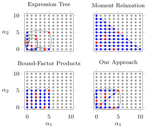 Figure 1
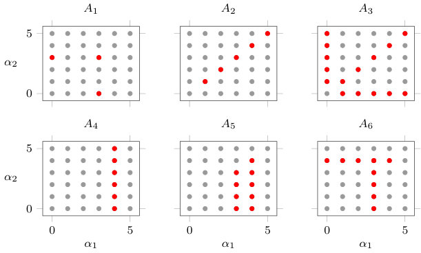 Figure 2
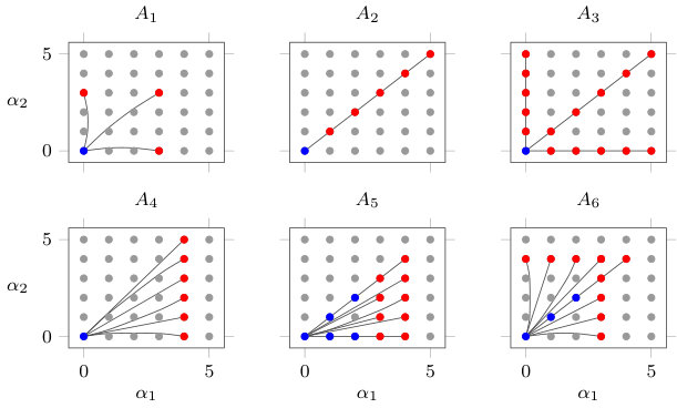 Figure 3
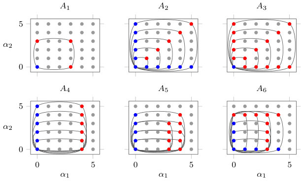 Figure 4
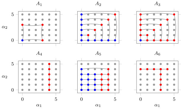 Figure 5
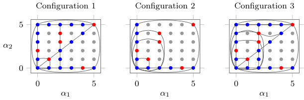 Figure 6
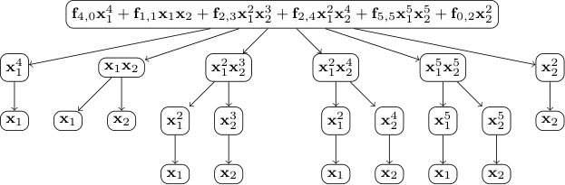 Figure 7
 Figure 8
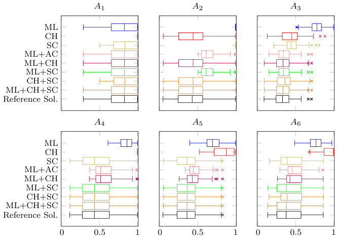 Figure 9
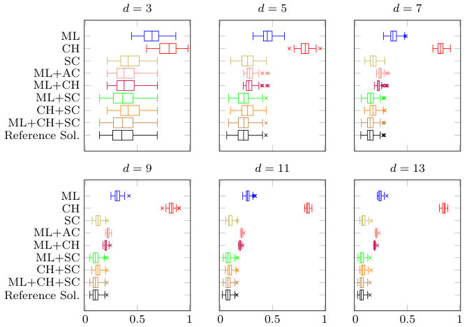 Figure 10
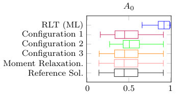 Figure 11
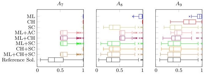 Figure 12
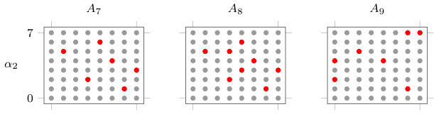 Figure 13
| Label | Description |
|---|---|
| (B) | Reference solution: To approximate we use the best upper bound for and the best lower bound for that BARON returns within a CPU time limit of seconds each. |
| (R) | Root node relaxation of the BARON solver. |
| (CS) | Reference solution obtained from solver CS-TSSOS. |
| (Y) | Reference solution obtained from YALMIP’s sos method. |
| (SOS) | Self-implemented sos relaxation (that does not exploit sparsity) of the lowest hierarchy level. |
| (M) | Relaxation based on the multilinear patterns , which consists of the inclusion-maximal elements of |
| (S) | Relaxation based on a family of shifted chains , which consists of the inclusion-maximal elements of {η+CH(e^i,d) : d∈2N\{0}, η∈N^n, i∈[n]}, that satisfy and #(η+CH(γ,d))∩A¿ #(η+CH(γ,d-1))∩A. The latter conditions ensure that each shifted chains contains at least two exponents from and that we cannot include more exponents from if we choose a bigger . |
| (C) | Relaxation based on a family of chains , which consists of the inclusion-maximal elements of {CH(γ,d) : d∈2N\{0}, γ∈N^n}, that satisfy and |
| (MC) | Relaxation based on a family of multilinear patterns, chains and shifted chains, F^mc_A:= F^m_A∪F^c_¯A ∪F^s_~A where , . |
| (H) | Let and . A relaxation based on the family F^h_A: = {CH(γ,d(A)) : γ∈Γ}∪F^m_ {CH(γ,d(A)) : γ∈Γ}∪F^m_A, which uses chains that are linked by multilinear patterns to strengthen . |
| (T) | Let , and . A relaxation based on the family , which consists of the inclusion-maximal elements of {TS((e^i)_i∈supp(α),d_1) : α∈A\TS(Γ,d_2) }∪{TS(Γ,d_2)}. Here, is a matrix with columns . The family uses -variate truncated submonoids with to cover the exponents in and connects these chains using one -variate truncated submonoid. |
Peer Reviews
No public reviews on file for this paper yet. If you reviewed it on a platform where reviews are public (OpenReview, ICLR, NeurIPS, ICML), you can paste yours below so the community can read it here.
Videos
No videos yet. Explain this paper in a talk, walkthrough, or lecture? Add one.
Taxonomy
TopicsAdvanced Optimization Algorithms Research · Polynomial and algebraic computation · Numerical Methods and Algorithms
\newsiamremark
hypothesisHypothesis
\newsiamthmclaimClaim
\headersConvexification via monomial patternsA. Averkov, B. Peters, and S. Sager
\externaldocumentex_supplement
Convexification of box-constrained polynomial optimization problems via monomial patterns ††thanks:
\fundingThis work was funded by the the Deutsche Forschungs gemeinschaft (DFG, German Research Foundation) - 314838170, GRK 2297 MathCoRe.
Gennadiy Averkov Fakultät 1, Brandenburgische Technische Universität Cottbus-Senftenberg, Germany (). [email protected]
Benjamin Peters Fakultät für Mathematik, Otto-von-Guericke Universität Magdeburg, Germany (, ). [email protected]
Sebastian Sager33footnotemark: 3
Abstract
Convexification is a core technique in global polynomial optimization. Currently, there are two main approaches competing in theory and practice: the approach of nonlinear programming and the approach based on positivity certificates from real algebra. The former are comparatively cheap from a computational point of view, but typically do not provide tight relaxations with respect to bounds for the original problem. The latter are typically computationally expensive, but do provide tight relaxations. We embed both kinds of approaches into a unified framework of monomial relaxations. We develop a convexification strategy that allows to trade off the quality of the bounds against computational expenses. Computational experiments show very encouraging results.
keywords:
Convexification, McCormick envelopes, moment problem, nonlinear optimization, polynomial optimization, sum-of-squares, sparsity
{AMS}
68Q25, 68R10, 68U05
1 Introduction
Many important convexification techniques applied to polynomial optimization problems share the following common distinctive features: in the case of a problem in variables , monomials
[TABLE]
with are substituted with monomial variables and the relationships among them are captured, exactly or in a relaxed fashion, by systems of convex constraints. In order to describe the relationship between different monomial variables by constraints one needs to introduce additional auxiliary monomial variables.
Different approaches exist on how to pick these auxiliary monomial variables and the respective convex constraints. The “nonlinear optimization community” uses monomial variables and constraints such that the resulting relaxations are cheap to compute. The resulting poor lower bounds are compensated by solving many relaxations within a branch-and-bound framework. The “polynomial optimization community” usually aims to solve only one single relaxation, which often produces a very tight bound. This comes at the price of a large number of monomial variables and hard constraints. Interestingly, up to now there has been little interaction between the two different schools of thought. The authors believe that a major reason is the lack of a mathematical formalism that would allow a uniform description of different convexification techniques.
One contribution of this paper is the introduction of the notion of patterns to fill this gap. Patterns are finite sets of exponent vectors that are chosen in such a way that the monomial variables indexed by can be linked by constraints that satisfy a given demand on the computability. While various kinds of patterns have been implicitly used by the disjoint research communities, the introduction of the explicit notion of patterns allows for the development of a unifying mathematical language that highlights common ideas. Promoting the elementary notion of patterns enables to see similarities of the different research directions and will help to connect different communities that work independently on the same problems.
For example, the pattern corresponds to the well-known McCormick envelope [31, 7], i.e. the convexification of the variables and and their product . Other examples of methods that can be expressed using the notion of patterns are truncated moment relaxation and its dual the sum-of-squares relaxation [2, 21, 28], scaled-diagonally-dominant sums of squares [1], sums of non-negative circuit polynomials [13, 38], bound-factor products [10] and their dual Handelman’s hierarchy [17], multilinear intermediates [4], polyhedral outer approximations [43] as well as expression trees [40, 39]. We propose a flexible template for the relaxation of box-constrained polynomial optimization problems (pop) that allows to use the ideas of these until now largely disjoint schools of thought. It allows to combine different types of patterns to build convex relaxations of a pop. Our new and more general point of view might also help to understand numerical issues and the facial structures of feasible sets in the aforementioned convexification approaches. This, in turn, can be expected to have a positive impact on the improvement of existing and on the development of novel approaches to polynomial optimization.
We address in this paper the case of box-constrained pops. In nonlinear global optimization, convexification of expressions occurring in constraints and objective functions (with the underlying variables in specified finite ranges) is a widely used technique. Since objective functions and constraints can be convexified by the same principles, one could also use our strategy for more general versions of polynomial optimization, with more general sets of constraints. On the other hand, developing our strategy into a sound method for general polynomial optimization would require more thought and ideas. Therefore, this is out of scope for this paper. Furthermore, box-constrained subproblems are an essential part of branch-and-bound frameworks such as employed in BARON [36]. Thus, in the future one can also try to employ our method developed for box-constrained pops with more general constraints by using them within branch-and-bound frameworks.
We derive various new convexification techniques from the monomial pattern template. The resulting relaxations can be solved by a variety of different numerical approaches. In the interest of analyzing the tightness and computational expenses related to different convexification strategies, we use the interior point solver MOSEK.
The paper is organized as follows. The basic notation is given in Section 2. In Section 3 the notion of the pattern relaxation is introduced and the separation problem for patterns is formulated as an optimization problem. Section 4 is dedicated to the interpretation and discussion of established convexification techniques as monomial patterns. Multilinear envelopes are generalized as multilinear patterns. In Section 5 new pattern types are introduced, which give rise to new algorithmic approaches to pop. Computational results in Section 6 highlight the benefits of our novel approach. Finally, a conclusion is given in Section 7.
2 Basic Notation
is the set of natural numbers including zero. For integers and we define , and . Let be nonempty, finite sets with cardinalities and . We denote vectors of real numbers with entries indexed by the elements of set as . Note that is isomorphic to . We define the bilinear product of two such vectors and as
[TABLE]
Furthermore, if , we define the coordinate projection of onto components indexed by as The and norms of are and , respectively. Let be a nonempty and compact set. We call
[TABLE]
the diameter of and
[TABLE]
the width function of in direction . We define the support of a vector and the support of a set as
[TABLE]
is said to have full support if . The standard basis vectors of are denoted by for and the all ones vector by . is the ring of polynomials in a vector of intermediates and the set of polynomials . That is, by we prescribe which monomials can occur in . The vector is called the coefficient vector of . The monomial support of a polynomial is . A polynomial is called sum-of-squares (sos), if for finitely many polynomials . We use to denote the cone of -variate sos of degree at most . The -truncated moment vector map is
[TABLE]
The minimum and maximum of the monomial , over a compact set are
[TABLE]
respectively, and The degree of the set is For vectors we understand notions like componentwise. Let with , we define the box as We use to abbreviate positive semidefinite.
3 Pattern Relaxation
3.1 Monomial Convexification and Monomial Relaxation
Let be a finite and nonempty set and be given. We consider the problem of minimizing a polynomial over the box , i.e.
[TABLE]
Via lifting, we reformulate (4) as an optimization problem in with a linear objective:
[TABLE]
Replacing the feasible set by its convex hull yields the monomial convexification of (4):
[TABLE]
We refer to as a (-variate) moment body. Clearly, the convexification (8) of (4) is tight, that is, the optimal values of (8) and (4) coincide. For general sets , the constraint is difficult to verify. Thus, it is natural to relax to a system of simpler constraints of the same type
[TABLE]
where is a finite family of finite subsets of that satisfies
[TABLE]
Our intention is to cover by sets such that the corresponding moment bodies yield more structure that we can exploit algorithmically than the original moment body . We call a pattern and (9) a pattern relaxation of with respect to the pattern family . Throughout the paper we use to denote and refer to as original exponents and to as auxiliary exponents. Using a pattern relaxation of we obtain a lower bound on (4) by solving
[TABLE]
An advantage of this approach is that we can choose patterns such that the computational costs of solving (possibly several instances of) (14) and the obtained lower bounds on the objective function value of (4) are well balanced.
This procedure can also be seen as embedding into for some set that contains and can be represented nicely as a union of patterns . Geometrically, the passage from (4) through (8) to (14) can be represented by the diagram
[TABLE]
The quality of a pattern relaxation of with respect to the family of patterns depends on how the moment variables are connected by the system of conditions (9). We say that monomial variables are directly connected by if holds for some . Furthermore, are indirectly connected by if there exist , such that and for all .
4 Known Convexification Techniques are Monomial Patterns
We formulate established convexification techniques from the literature as monomial patterns. These pattern types can be used – alone or in combination – to generate computationally tractable pattern relaxations (14) of (4).
4.1 Multilinear Pattern
Let , and . We call
[TABLE]
a multilinear pattern (ML), see subplot in Fig. 1 for an illustration. It is well known that the convex envelope of multilinear functions over is a polytope. In our context this implies the following.
Proposition 4.1**.**
Let be of full support. The moment body is a polytope satisfying
[TABLE]
*with . *
Multilinear patterns can be found in different contexts in the literature. In their basic version they are used to convexify multilinear polynomials. An essential building block for the convexification of product terms is the McCormick envelope [30], that is the convexification of bilinear products by a tight description of the moment body , noting that . McCormick envelopes have been successfully used to build convex relaxations of multilinear monomials by applying them recursively. For a monomial with and this recursion can be described as follows. Let and . For each element write as with . Remove from and add to if respectively to if . Add the multilinear pattern to . This procedure corresponds to a binary tree with root and the moment body of each pattern in is tightly described by a McCormick envelope.
In general it is not clear how to favorably decompose a multilinear exponent . For the smallest nontrivial case this has been investigated in [41].
Another way to convexify with and is to introduce for each factor with a moment variable [11]. This corresponds to the pattern
[TABLE]
For the pattern relaxation corresponding to the pattern family is tight, while relaxation corresponding to is usually not tight for . It is however not clear which system
[TABLE]
or
[TABLE]
yields a tighter convex relaxation of for with . This is due to the different choice of auxiliary variables and how the original moment variables are connected by the different pattern families. In our definition (15), the parameter allows to flexibly choose auxiliary variables and thereby control the connective properties of the multilinear pattern family.
Multilinear patterns have also been applied to general polynomials with and [4, 16]. Using the set , the substitution and a multilinear intermediate of is generated. This corresponds to relaxing the usually non-polyhedral with the polytope and
[TABLE]
(22) is further relaxed using (18) or (17). The entire process can be expressed using multilinear patterns as well. For example using (17) to further relax (22) yields the family .
Example 4.2**.**
We consider different exponent sets for in the following,
[TABLE]
*The exponent sets and different patterns are visualized in Figures 1, 4, and 5 as follows. The title of a subplot refers to the set of original exponents which are depicted by red squares. The auxiliary exponents are depicted by blue dots. A pattern corresponds to an undirected smooth curve and all the colored points and squares that the curve passes through. will also be used in the numerical result section. *
4.2 Expression Trees
Convexification using expression trees is common in general nonlinear optimization [39, 40]. This approach is based on the observation that each algebraic expression is made up of a certain set of elementary operations, such as powers, linear combinations, or products of expressions. A decomposition of an algebraic expression into these operations can be visualized using an algebraic expression tree, like in Fig. 2. This is a rooted tree with nodes labeled by terms occurring in the expression. Each term is built up from its child terms using elementary operations and the underlying convexification is obtained by introducing a variable for each node and providing convex constraints that link every node and its child nodes. For polynomials, given as a linear combination of monomials, all the nodes apart from the root node correspond to monomial variables. A non-root node and its child nodes therefore build a pattern.
For example, the term in Fig. 2 is decomposed into the product of the powers and of the variables and . For these three terms, one introduces the monomial variables , and , respectively. The relationship of these variables is captured by the pattern and the corresponding moment body is described by the well-known McCormick inequalities. The variable is further connected to by exponentiation. The corresponding pattern is . All patterns induced by the tree in Fig. 2 are visualized in the first subplot of Fig. 3. Observe that there other ways to form expression trees. For example one could also decompose into and . However, the corresponding pattern is no longer tightly described by McCormick inequalities.
Since expression trees normally correspond to patterns of small size, they lead to weak, but efficiently computable relaxations, which are often used in divide-and-conquer approaches like branch-and-bound.
4.3 Bound-Factor Products
Another convexification approach is based on so-called bound-factor products (BF) [10]. Since the polynomials and are nonnegative on , the products of these polynomials (with repetitions allowed) are also nonnegative on . So, one can consider the products
[TABLE]
of polynomials with linear factors depending on the variable , where and . For a generic choice of and , the polynomial includes all monomials with exponents in the pattern . By substituting for all we obtain a linearization of . The system of linear inequalities
[TABLE]
is valid for . This approach can also be viewed as hierarchical since one can increase the order of the bound-factor products in order to tighten the relaxation. Note that in polynomial optimization this approach is known as the dual of Handelman’s hierarchy [17]. Within this approach one groups monomial variables into patterns of a rather large size and connects them with only linear constraints. For example, to generate a non-trivial relaxation of (4) using bound-factor products for the set from Example 4.2 one is forced to use at least one pattern with and , which means that at least monomial variables have to be introduced, compare Fig. 3. Another issue is that the system of linear inequalities (24) is not a tight description of . These kinds of relaxations have also been used within branch-and-bound strategies [10].
4.4 Moment Relaxation
The most popular convexification techniques in the polynomial optimization community are the moment relaxation and its dual counterpart, the sos relaxation [2, 21, 28]. This approach introduces a large number of monomial variables and links them all with one large pattern using psd constraints. The approach is hierarchical in the sense that one first needs to choose a bound on the degree of the monomials, for which monomial variables are introduced. These hierarchies have in practice good approximation properties at the expense of large sdps, see [33] for computational studies. Even though the lowest possible hierarchy level of the moment relaxation often produces tight bounds, it does not scale well when the number of variables and/or degree grows. However, strategies exist to make the approach more tractable, e.g., exploiting correlative sparsity [45, 24, 23, 18, 27], term sparsity and structures of the Newton polytope [34, 48], combinations of the previous [47, 49], symmetry structures [35, 2] as well as spectral methods that exploit the so-called constant trace property of sos hierarchies [26].
To derive a so-called moment relaxation of (4), the following representation of the moment body in terms of probability measures is used:
[TABLE]
So a vector belongs to iff there exists a probability measure on such that for all . Hence, (8) can be formulated as
[TABLE]
In pursuit of a tractable characterization of the feasible set, we use the following definition and theorem.
Definition 4.3** (Moment Matrix and Localizing Matrix [20, Ch.2.7.1]).**
The localizing matrix for a polynomial with coefficients and the moment matrix are defined as
[TABLE]
Theorem 4.4** ([20, Th. 2.44]).**
Let be -variate polynomials such that there exist sos polynomials for which
[TABLE]
is compact. Furthermore, let A sequence has a finite Borel representing measure with support in iff
[TABLE]
We describe the box by the polynomials for , i.e. . Clearly, the assumptions of Theorem 4.4 hold and we can formulate (8) as
[TABLE]
The moment and localizing matrices from the above constraints are submatrices of infinite matrices with rows and columns indexed by rather than . Thus, since is arbitrarily large, the constraints can be viewed as infinite-dimensional psd constraints that impose semidefiniteness of the infinite moment matrix and infinite localizing matrices. By fixing a particular one relaxes the infinite dimensional psd problem to a finite-dimensional one. This is known as the choice of the level of the hierarchy of the moment relaxations. It is natural to restrict attention to levels that are sufficient large to ensure that all the variables occurring in the objective function appear in the constraints. Thus, for every , we consider the optimal value of the semidefinite problem
[TABLE]
The value is a lower bound on the optimal value of (4). This problem has one sdp constraint of size that involves the monomial variables , and sdp constraints of size that involve . Hence, the moment relaxation corresponds to the pattern . Note that for general problems it is not possible to reduce the size of the mentioned sdp constraints [3]. For a small example like Example 4.2 with and this adds up to 66 moment variables. The third subplot in Fig. 3 shows the pattern corresponding to the lowest hierarchy level which involves an sdp constraint with a matrix.
4.5 Singletons
The smallest patterns are singletons with . The moment body of a singleton is the interval . The pattern relaxation of induced by the family of singletons is . This is the weakest possible relaxation within the pattern approach. The provided bounds on the monomial variables can be exploited by branch-and-bound solvers [36].
4.6 Alternative Techniques
Besides the mentioned techniques there exist other approaches for polynomial instances. For example approaches based on geometric programming or relative entropy relaxations for signomial programming have been investigated in [14, 15, 9, 8]. Closely related to geometric and signomial programming are special non-negativity certificates utilizing so-called sums of nonnegative circuit polynomials (sonc) [13, 38, 25]. Note that the cones of nonnegative circuit polynomials are essentially power cones. As it is well known that these cones have second oder cone lifts, so does the sonc cone. For a different proof see [46]. Furthermore, in [12] the authors purpose a linear approximation of the sonc cone.
Another approach uses scaled diagonally dominant sums of squares (sdsos) [1], that is a non-negativity certificate based on sos polynomials with sparse monomial support with .
By dualizing the sonc [19] and sdsos relaxations, one arrives at convexifications in terms of monomial variables. These duals correspond to pattern relaxations that use special pattern types, see an illustration in Fig. 4 for the case .
5 Truncated Submonoids
In order to generate computationally tractable relaxations of (4) we look for patterns such that we can formulate the constraint of (14) (or a sufficiently tight approximation of this constraint) in such a way that it is accessible to optimization methods. In this section we introduce the new pattern type truncated submonoids for which we determine the size of these constraints.
Let , and be a matrix, whose columns are nonzero vectors with pairwise disjoint supports. Clearly, such vectors are linearly independent. We call
[TABLE]
the -variate -truncated submonoid (TS) and its generators.
Proposition 5.1**.**
The moment body can be represented as a -variate moment body by
[TABLE]
Proof 5.2**.**
*The desired representation is obtained by taking the convex hull of the left and the right hand side of the equality . *
The next proposition follows by combining Theorem 4.4 and Proposition 5.1.
Proposition 5.3**.**
Let for each Then if and only if there exists with for all and
[TABLE]
Using Proposition 5.3 we can treat the constraint as in the moment relaxation, i.e., truncating the infinite dimensional matrices at an even with . Naturally, the complexity of the constraints (41) depends and . For practical purposes, it is desirable to choose these parameters not to large. We use , truncating the matrices in (41) at , because of several reasons.
- •
Since our overall strategy for (4), based on (14), does not guarantee determination of the exact optimal value of (4), we see no need in exact approximation of the constraints in (14) at high computational costs. Therefore, when is a truncated submonoid pattern, we prefer to relax by means of Proposition 5.3 using a value that is not too large.
- •
The lowest possible level of the moment relaxation often yields sufficiently tight bounds.
We would like to stress that in practice the size of moment relaxations for the original problem (4) does not scale well if the degree of and grows. In general it is not possible to reduce this size if does not admit any specific sparsity structures; see [3] for a theoretical justification. In contrast, we believe that one can use moment relaxations for the constraint , since we can keep the size of the matrices in (41) under control.
5.1 Chains
For and , we call
[TABLE]
a chain. A chain is a special truncated submonoid pattern with . In the case of chains , the constraints of (14) amounts to semidefinite constraints.
Theorem 5.4** ([21, Th. 3.23]).**
Let be an nonnegative integer, with and Then
[TABLE]
Combining Proposition 5.1 and Theorem 5.4 we obtain:
Proposition 5.5**.**
Let be a chain pattern and Then the moment body can be represented using semidefinite constraints
[TABLE]
5.2 Shifting a Pattern
To generate new patterns by shifting existing ones by a vector , we can use the following proposition.
Proposition 5.6**.**
Let be a pattern with and a vector with . Then
[TABLE]
Proof 5.7**.**
The assertion follows from and the observation that and have no common factor since . Hence
[TABLE]
5.3 Shifted Chains
We apply the shifting procedure to chains and generate a new pattern type. Let and with . We call a shifted chain. Using Proposition 5.6 we can represent the moment body as the convex hull of and and formulate a result for shifted chains in analogy to Proposition 5.5.
Corollary 5.8**.**
Let have disjoint support and an integer. Let . Then if and only if there exists such that
[TABLE]
5.4 Generalizing Truncated Submonoids
It is possible to expand the notion of truncated submonoids to generators by using the shifted truncated submonoids with such that
[TABLE]
For different choices of the parameters , and sets one can apply Positivestellensätze that yield tractable characterizations of . For example let and be matrices whose columns have pairwise disjoint support and satisfy (42). Then from [28, Hilbert 1888] it follows that , and can be represented by psd constraints of size , and , respectively. Furthermore, if satisfies (42), then can be characterized by two psd matrices, one of size , one of size . In particular, combining these representations of and leads to a generalization of the underlying pattern of the sdsos certificate. At last, if satisfies (42), then can be characterized using at most two psd matrices of size at most . For that one has to determine whether the closure of is , a semi-infinite interval, the union of two disjoint semi-infinite intervals or a bounded interval and then apply the respective Positivestellensatz: [28, Hilbert 1888], [28, Stieltjes 1885], [28, Hausdorff 1921] or [28, Svecov 1885]. However, since we do not use any of these representations in the computations section, we do not pursue these patterns any further.
6 Computational Results
Finding an unbiased setting to compare the advantages and disadvantages of convex relaxations for pop is not trivial, as models, their purpose, and methods are usually closely linked to one another. We decided to use a prototype implementation to compute solutions of (14) for different monomial pattern families. The solutions are used to approximate the size of the relaxations, and compared on a new benchmark library of random pop instances among another and to results from BARON, YALMIP and CS-TSSOS. We start by describing implementation and comparison details, before numerical results for different classes of instances are discussed.
6.1 Implementation Details
Four different solvers were run for the numerical evaluation on a compute server with 4 Intel(R) Xeon(R) Gold 6138 CPUs with 20 cores of 2 threads and 1 TB RAM each under Ubuntu 18.04.4. Each solver-instance pair was assigned to one such job, i.e. the solvers themselves did not use the parallel structure. In order to distribute the solver-instance pairs to the 80 cores we used [42]. We used MATLAB 9.6.0.1174912 (R2019a) Update 5 [29], MOSEK 9.2.32 [32], JULIA 1.5.2 [6], CS-TSSOS version 1.00 [47], BARON 1.8.9 [43], and YALMIP 20200930 [22]. All reported run times are wall-clock times. The code for solving the pattern relaxation (14) was implemented and run in MATLAB and consists of roughly 3500 lines of code and uses MOSEK to solve the relaxations. The reported time is the termination time obtained from MOSEK. BARON [43] was called from MATLAB with default settings. BARON currently only returns the CPU time, when its MATLAB interface is used. Hence, we timed BARON calls with MATLAB’s tic and toc commands111This method was suggested with the support of BARON.. CS-TSSOS is a JULIA package that allows to exploit correlative sparsity and term sparsity simultaneously. We called the first level of the hierarchy by running the command cs_tssos_first with settings order and TS="MD". CS-TSSOS does not report the time of the solution process. Thus, we first piped the output from the sdp solver MOSEK, that CS-TSSOS uses, to a text file. After that we read the termination time of MOSEK from the text file. Since only two decimal places are obtained this way, the time we report is only a proxy of the time of CS-TSSOS’s actual MOSEK call. YALMIP is a MATLAB toolbox that allows to compute the moment as well as the sos relaxation of (4). We run YALMIP’s solvesos lowest possible level of the sos hierarchy and report the termination time obtained from MOSEK.
6.2 Setup of Numerical Comparisons
As an indicator for the tightness of relaxations we approximate the size of feasible sets by their width. For a given finite and nonempty set and a vector we define the width function of in direction as
[TABLE]
Replacing by a relaxation based on a pattern family one obtains an upper bound on the value of , denoted by . The evaluation requires solving two instances of (14) for every pattern of interest, using the objective functions and , respectively. To normalize the values and , we divide by the width function obtained for the (trivial) relaxation using the singletons-only pattern , i.e.,
[TABLE]
Table 1 lists the methods and patterns that were used for the numerical results. Method (B) gives an approximation of the reference solution, albeit at a high computational cost. (R) can be seen as the current state-of-the-art for a relaxation within a divide-and-conquer approach. Our approach allows to compare the new relaxation strategies (M), (C), (MC), (H), (T) with respect to the width function.
Figs. 7, 8, 9, 10, and 12 show box plots of our numerical findings. The box plots visualize the distributions (20 random vectors ) of the normalized width functions (44) for various methods from Table 1 computed with BARON, YALMIP and CS-TSSOS. The title of a subplot corresponds to the exponent set . Below the method (see Table 1) the rounded mean time in seconds is shown for the respective method. The box borders are the and the -quantiles. The lower whisker is the smallest data value which is larger than the lower quartile times the interquartile range and the upper whisker accordingly.
6.3 Test Instances
In our test instances, we use 13 finite exponents sets classified into four types: specially structured adversary sets, dense sets, sparse sets, and the example from above. They are explained in the next subsection. For each exponent set we chose and 20 (uniform distributed) random coefficient vectors . The instances were a priori filtered to avoid trivial problems. If BARON did terminate on both the minimization and the maximization tasks in (43) within the CPU time limit of 1000 seconds, the instance was replaced. Therefore the corresponding mean times for (B) are always at least seconds.
Our approach to generation of test instances is a search for instances that are interesting and realistic enough, on the one hand, but computationally challenging for the existing methods, on the other hand. That is, we wanted to study if existing convexification strategies can be improved on some interesting families of optimization problems.
While we test our approach for (4) on the unit box and with the objective functions having coefficients in , our approach is applicable without any changes for general objective functions and on arbitrary axis-aligned boxes. We also expect that the results of our numerical evaluations would be the same in this slightly more general setting.
6.4 Numerical Results
In this subsection we describe the different exponent sets and present numerical results for the different methods from Table 1.
6.4.1 Adversary Exponent Sets
If a pattern family yields poor connectivity properties for an exponent set, we consider this set to be an adversary exponent set for this family. In subplot from Fig. 1, for example, we see that the sparse family of multilinear patterns connects none of the original exponents. Hence, chain shaped exponent sets are natural adversaries for relaxations that only use multilinear patterns. As a result, the first two subplots in Fig. 7 show that the bounds using (M) coincide with the bounds obtained by the weakest pattern family . On the other hand, it is not surprising that the bounds obtained by using one chain (C) match the reference solution (B). The sparsity exploiting solver CS-TSSOS as well as YALMIP’s sos method fail to terminate for any of the 20 instances with exponent set . We suspect that the reason for this is that does not yield any term or chordal sparsity structures that can be exploited. Thus, CS-TSSOS and YALMIP solve a regular sos relaxation for and , involving an sdp with a psd matrix.
Another adversary exponent set for multilinear patterns is . It can be covered sparsely by multilinear patterns using the family . Each pattern of connects original exponents, but establishes no connection between monomials from different patterns. That is because two patterns with satisfy . The poor connective properties of explain their poor performance, see (M) in Fig. 7. By additionally using chains to connect the multilinear patterns, the family exploits the structure of . As a result, the resulting bounds of (H) and (B) are indistinguishable in Fig. 7. Again, CS-TSSOS and YALMIP fail to terminate for any of the instances with exponent set – most likely for the same reason as above.
6.4.2 Dense Exponent Sets
We consider dense exponent sets for and . The pattern families shown in Fig. 8 perform reasonably well, probably due to their connectivity properties. Furthermore, we see that the multilinear patterns (M) perform for drastically better than (R). This might be because the multilinear patterns used in are bigger than the ones BARON uses, leading to more connections between monomial variables.
6.4.3 Sparse Exponent Sets
We use randomly generated sparse exponent sets to test pattern families that do not assume any structure of . is generated by randomly picking exponents via randperm from .
Fig. 9 column (M) shows that does not perform particularly well. Column (H) shows that additionally enforcing indirect connections between moment variables via chains and multilinear patterns in results in tighter bounds.
Fig. 10 shows the distribution of the width for sparse instances with a high number of variables and low degree . Computing lower bounds for the instances using relaxations that do not exploit sparsity of involves severe computational cost. We ran into memory problems with YALMIP for the instance with when . Thus, we used (SOS), that is an own implementation of an sos relaxation instead. (The method (SOS) yields similar bounds to (Y) for with average times s and s). Interestingly, the bounds computed by CS-TSSOS are worse than the ones ones computed with the pattern family . It might be that using different settings for CS-TSSOS yields better bounds. However, this would also result in higher computation times. The pattern strategy (T) yields for all tested nontrivial bounds. Note that for these bounds seem to be reasonably tight, when compared to (Y) or (SOS), but for a fraction of the computation time.
We want to point out that we were able to compute nontrivial bounds for instances with exponent sets . For these exponent sets the computation of one of the two optima involved in the definition of the width usually takes between 6-7 minutes. The reason for the good performance in terms of computation time of (T) can be traced back to the relatively small size of the biggest involved psd matrices in the relaxation of (14). That is for
[TABLE]
For and this boils down to \mathrm{r}\leq\max\Big{\{}\tbinom{2+4}{4},\tbinom{1+\mathrm{n}}{\mathrm{n}}\Big{\}}.
6.4.4 Custom Strategies
A customized pattern family for a given exponent set allows to trade off computational cost versus tightness of the relaxation. Figure 11 shows three example pattern families customized for from Example 4.2.
While the bounds obtained from , see in Fig. 12, are far from optimal, they are an improvement compared to in producing bounds similar to those obtained by (B).
7 Conclusion
We have presented a customizable framework for the relaxation of polynomial optimization problems over a box that is based on monomial patterns. This framework allows inclusion and combination of existing approaches that were developed by different communities. In fact, various kinds of linearizations of multilinear terms, relaxations based on bound-factor products, dual versions of the relaxations of polynomial optimization problems based on sos, sdsos and sonc polynomials all come with their particular type of pattern. The advantage of our approach is that by using patterns we can exploit the combinatorial structure of the set of monomial exponents. This is done by covering the monomial support with a pattern family that reflects the structure of . Using patterns, we are able to avoid hard problem formulations by neglecting dependencies between certain monomials and instead focus on well-behaved and easy-to-describe dependencies between certain other monomials. The results were high-quality and tractable relaxations of (4).
Our computational experiments provided numerical evidence for the benefits of using different generic as well as customized pattern relaxations.
These computed bounds could be further improved by techniques within divide-and-conquer frameworks such as BARON [43], SCIP [44], COUENNE [5] or LINDOGlobal [37], in a similar manner as already done with McCormick envelopes in the global optimization community.
In particular, the more involved -variate truncated submonoids and its possible generalizations provide a way to use sos or moment methods to solve problems with polynomials of higher degree and with more variables. Choosing an appropriate set of generators of a truncated submonoid pattern, this pattern type could be used as an interface to combine sos methods with divide-and-conquer frameworks. Furthermore, combining truncated submonoids with sparsity exploiting approaches such as chordal or term sparsity pose a way to further improve the run times.
The numerical results also suggest that the connectivity properties of a pattern family have a major impact on the quality of the computed bounds. This could be further investigated and exploited with hypergraph based approaches in the future.
How to efficiently generalize the approach to polynomial inequalities and to identify properties of instances in specific application areas that might benefit particularly from the new approach, are further open research questions.
The reference list from the paper itself. Each links out to its DOI / PubMed record.
- 1[1] A. A. Ahmadi and A. Majumdar , Dsos and sdsos optimization: more tractable alternatives to sum of squares and semidefinite optimization , SIAM Journal on Applied Algebra and Geometry, 3 (2019), pp. 193–230.
- 2[2] M. F. Anjos and J. B. Lasserre , eds., Handbook on semidefinite, conic and polynomial optimization , vol. 166 of International Series in Operations Research & Management Science, Springer, New York, 2012, https://doi.org/10.1007/978-1-4614-0769-0 , https://doi.org/10.1007/978-1-4614-0769-0 . · doi ↗
- 3[3] G. Averkov , Optimal size of linear matrix inequalities in semidefinite approaches to polynomial optimization , SIAM J. Appl. Algebra Geom., 3 (2019), pp. 128–151, https://doi.org/10.1137/18M 1201342 , https://doi.org/10.1137/18M 1201342 . · doi ↗
- 4[4] X. Bao, A. Khajavirad, N. V. Sahinidis, and M. Tawarmalani , Global optimization of nonconvex problems with multilinear intermediates , Mathematical Programming Computation, 7 (2015), pp. 1–37.
- 5[5] P. Belotti , Couenne, an exact solver for nonconvex minlps , 2015, https://projects.coin-or.org/Couenne/ .
- 6[6] J. Bezanson, A. Edelman, S. Karpinski, and V. B. Shah , Julia: A fresh approach to numerical computing , SIAM Review, 59 (2017), pp. 65–98, https://doi.org/10.1137/141000671 . · doi ↗
- 7[7] N. Boland, S. S. Dey, T. Kalinowski, M. Molinaro, and F. Rigterink , Bounding the gap between the mccormick relaxation and the convex hull for bilinear functions , Mathematical Programming, 162 (2017), pp. 523–535.
- 8[8] V. Chandrasekaran and P. Shah , Relative entropy relaxations for signomial optimization , SIAM J. Optim., 26 (2016), pp. 1147–1173, https://doi.org/10.1137/140988978 , https://doi.org/10.1137/140988978 . · doi ↗