Perfect Sampling for Gibbs Point Processes Using Partial Rejection Sampling
Sarat B. Moka, Dirk P. Kroese

TL;DR
This paper introduces a perfect sampling algorithm for Gibbs point processes, leveraging partial rejection sampling, with efficiency depending on interaction range and point intensity.
Contribution
It develops a novel perfect sampling method tailored for specific Gibbs point processes with finite interaction range, improving sampling efficiency.
Findings
Expected running time scales as O(log(1/r))
Algorithm effective for moderate point intensities
Applicable to pairwise interaction, penetrable spheres, and area-interaction models
Abstract
We present a perfect sampling algorithm for Gibbs point processes, based on the partial rejection sampling of Guo et al. (2017). Our particular focus is on pairwise interaction processes, penetrable spheres mixture models and area-interaction processes, with a finite interaction range. For an interaction range of the target process, the proposed algorithm can generate a perfect sample with expected running time complexity, provided that the intensity of the points is not too high.
Click any figure to enlarge with its caption.
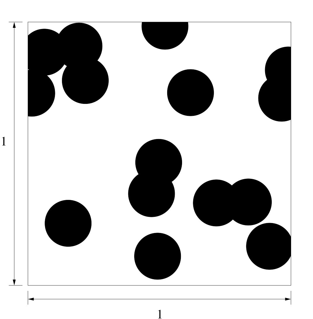 Figure 1
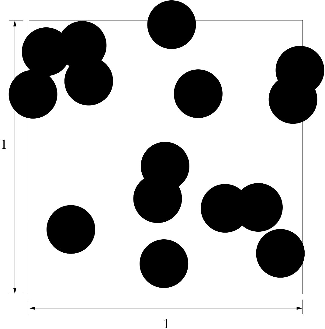 Figure 2
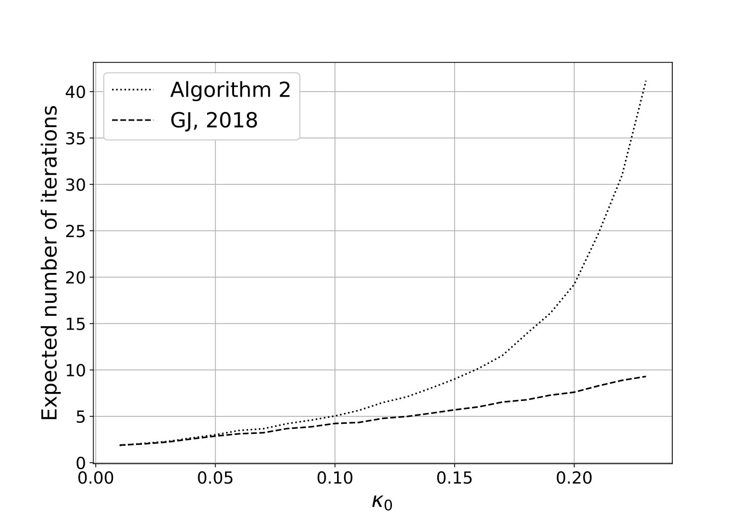 Figure 3
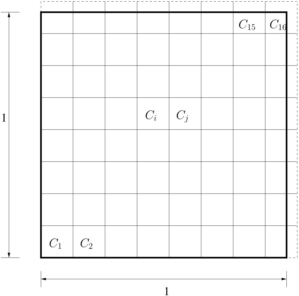 Figure 4
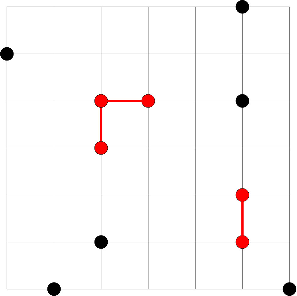 Figure 5
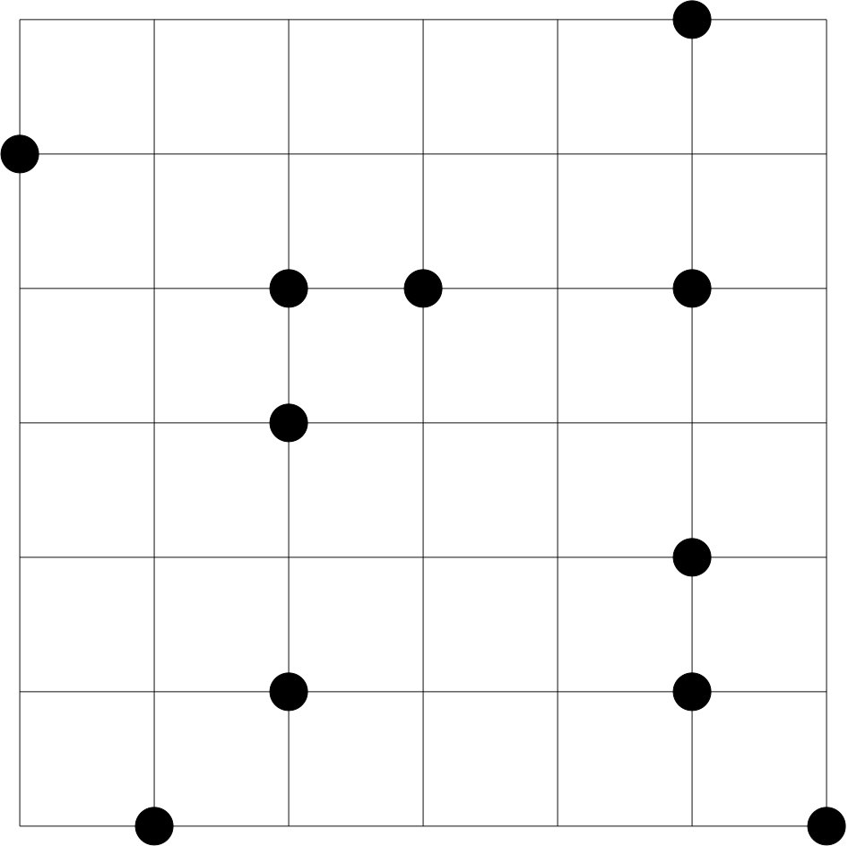 Figure 6
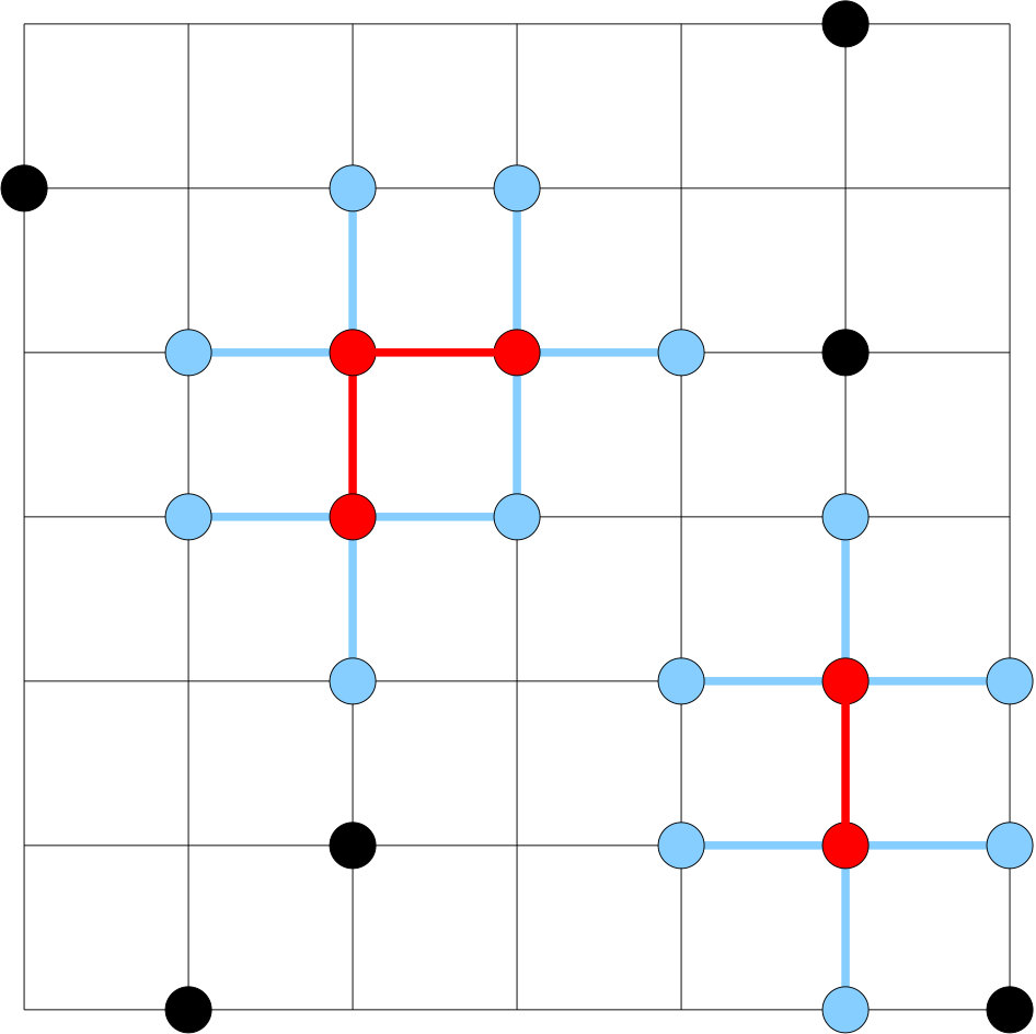 Figure 7
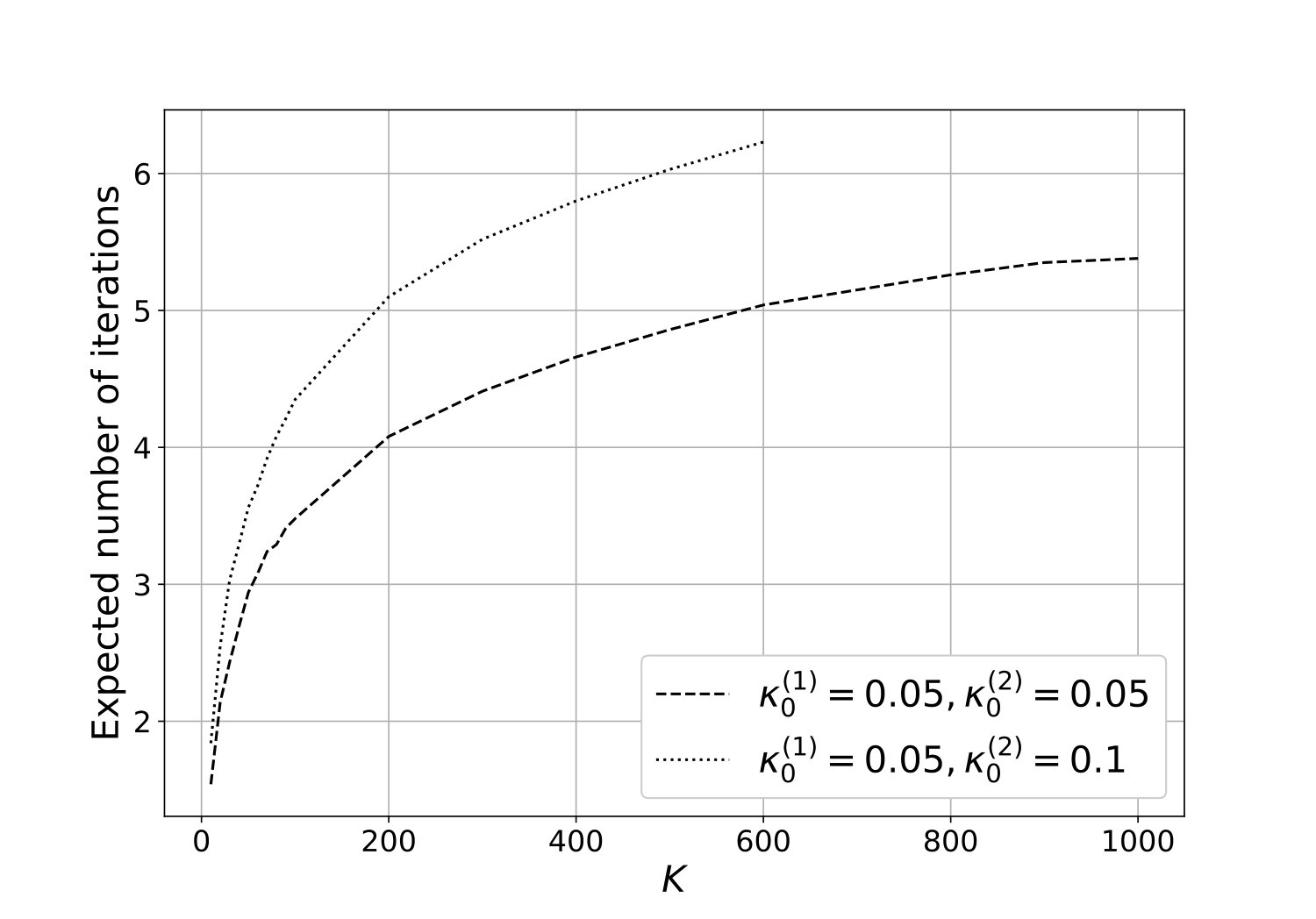 Figure 8
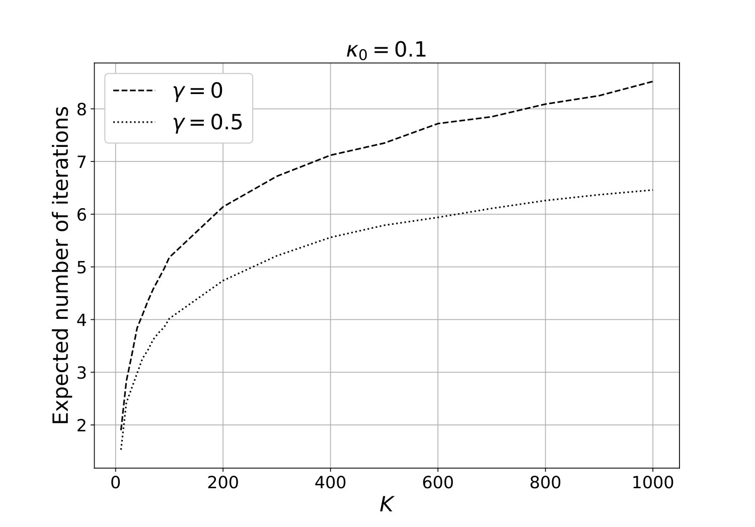 Figure 9
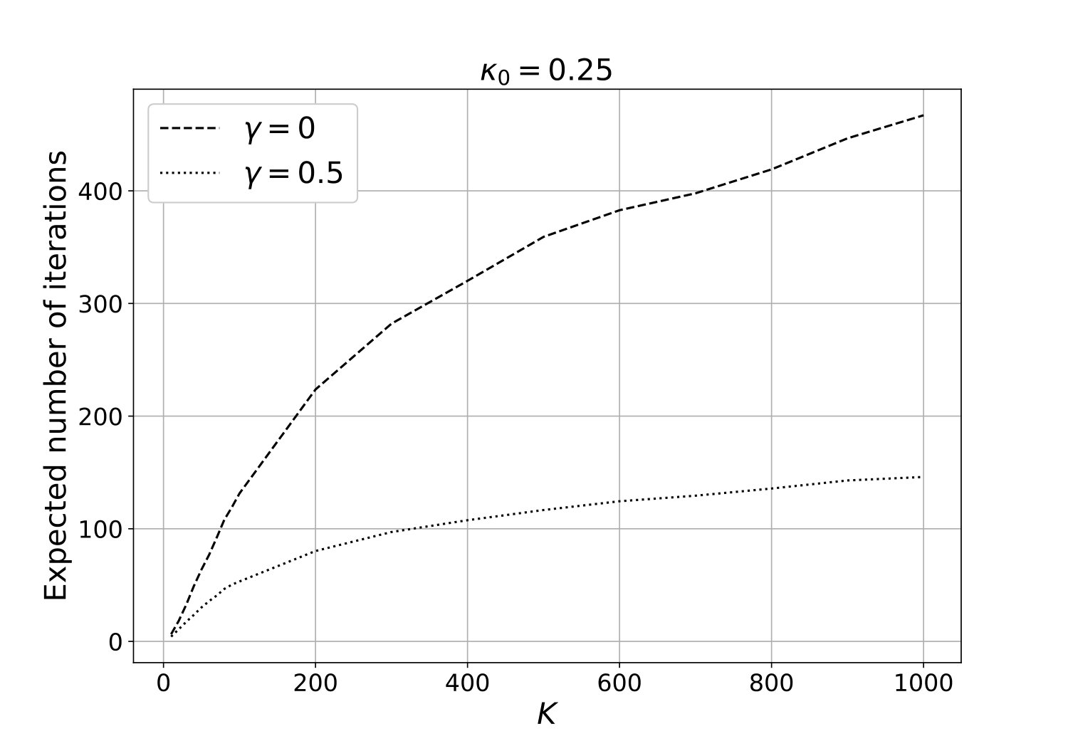 Figure 10
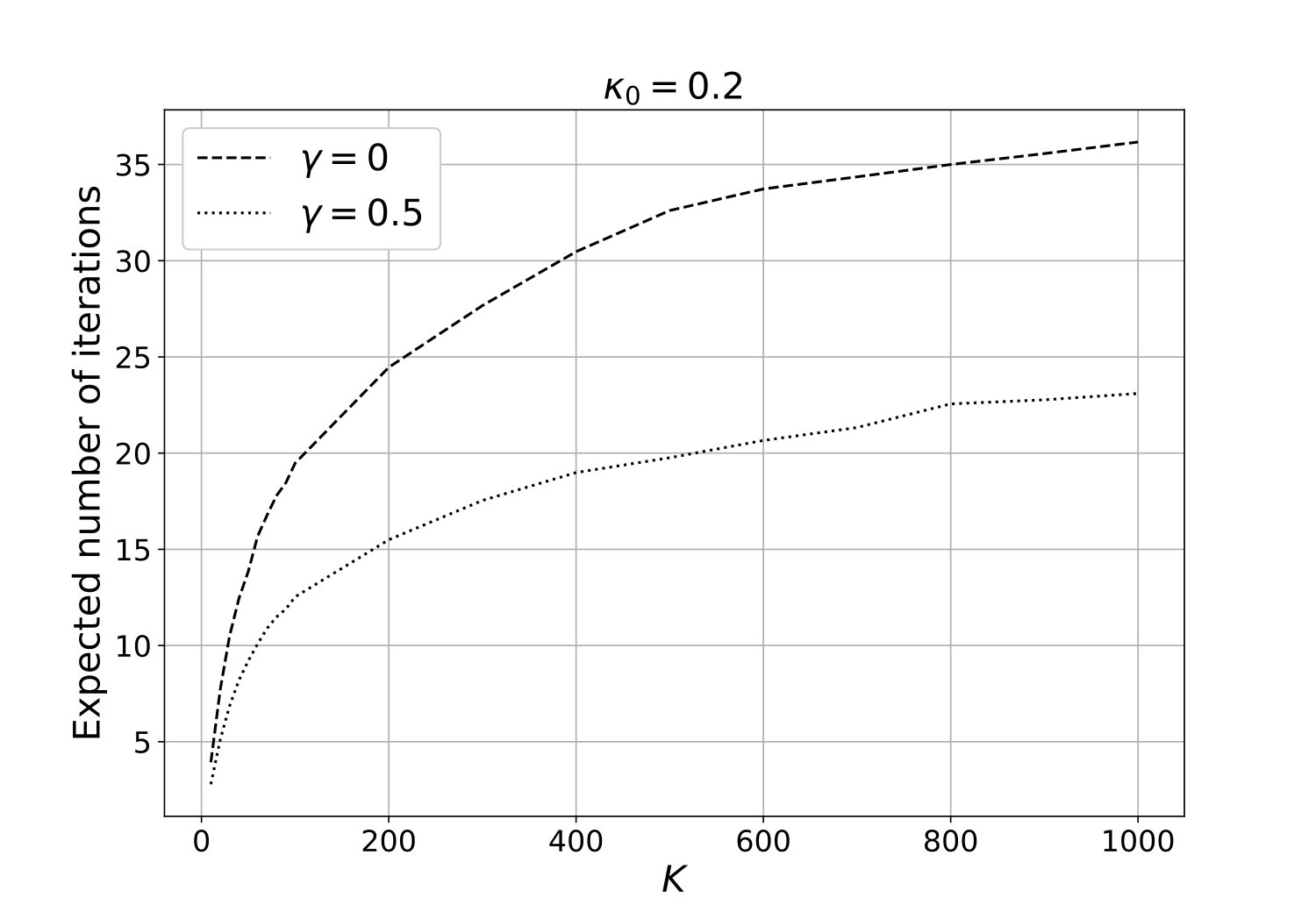 Figure 11
Peer Reviews
No public reviews on file for this paper yet. If you reviewed it on a platform where reviews are public (OpenReview, ICLR, NeurIPS, ICML), you can paste yours below so the community can read it here.
Videos
No videos yet. Explain this paper in a talk, walkthrough, or lecture? Add one.
Perfect Sampling for Gibbs Point Processes Using
Partial Rejection Sampling
Sarat B. Moka
School of Mathematics and Physics
The University of Queensland, Brisbane
Dirk P. Kroese
School of Mathematics and Physics
The University of Queensland, Brisbane
Abstract
We present a perfect sampling algorithm for Gibbs point processes, based on the partial rejection sampling of Guo et al., (2017). Our particular focus is on pairwise interaction processes, penetrable spheres mixture models and area-interaction processes, with a finite interaction range. For an interaction range of the target process, the proposed algorithm can generate a perfect sample with expected running time complexity, provided that the intensity of the points is not too high.
Keywords— Perfect sampling, Partial-rejection sampling, Hard-core process, Strauss process, Pairwise interaction process, Area-interaction process, Penetrable spheres mixture model
1 Introduction
Various phenomena in physics, chemistry and biology are modelled by Gibbs point processes. A Gibbs point process — or simply, Gibbs process — is a spatial point process whose distribution is absolutely continuous with respect to that of a Poisson point process (PPP). Pairwise interaction point (PIP) processes and penetrable spheres mixture (PSM) models are two widely studied examples of Gibbs processes; see, for e.g., Møller and Waagepetersen, (2004); Huber, (2016); Kendall and Møller, (2000); Baddeley and Nair, (2012); Baddeley and Turner, (2005). The PIP family includes hard-core processes and Strauss processes.
Perfect sampling for Gibbs processes is an active area of research. A sampling algorithm for a given distribution is called perfect if it generates an exact sample from this distribution within a finite time. We refer to Kendall, (1998); Fill, (1998); Kendall and Møller, (2000); Garcia, (2000); Ferrari et al., (2002); Huber, (2012); Moka et al., (2017); Guo and Jerrum, (2018) for some of the existing perfect sampling algorithms for Gibbs processes. The methods in Moka et al., (2017) and Guo and Jerrum, (2018) generate perfect samples of hard-core processes. The other methods in the references above are applicable to more general Gibbs processes, including PIP processes and PSM models. Among these methods, the dominated coupling from the past (dCFTP) methods by Kendall, (1998); Kendall and Møller, (2000) and Huber, (2012) are shown to be efficient when the density of the points is small; see, for example, Huber, (2016). As we show in this paper, for an interaction range of the target Gibbs process and dimension of the points, the expected running time complexity of any dCFTP method is at least of order even when the density of the reference PPP is very small. However, dCFTP algorithms are sequential and thus they do not take advantage of parallel computing. In this paper, we propose a method for generating perfect samples of PIP processes and PSM models using partial rejection sampling (PRS) method of Guo et al., (2017) and show how one can obtain, using parallel computing, an expected running time complexity of , provided that the density of the reference PPP is not too high.
The PRS method provides a general methodology for generating perfect samples from a product distribution, conditioned on none of a number of bad events occurring. Such problems are in general NP-hard; see, for e.g., Bezáková et al., (2016) and Guo et al., (2017). However, for certain types of parametric product distributions, the PRS algorithm is efficient and terminates within iterations on average, where is the number of bad events. An additional feature of the PRS algorithm is that, unlike the dCFTP methods, it is distributive, in the sense that it allows parallel computation within each iteration. As a consequence, the PRS algorithm can be implemented with expected running time complexity. By exploiting the distributive property of the PRS, we use the PRS algorithm for generating perfect samples of Gibbs processes on a Euclidean subset . In particular, a brief description of our contributions is as follows:
- •
We partition into a finite number of cells and define a product measure by ignoring the cross interactions between the cells. Further by defining appropriate bad events that depend on the cross interactions, we express the distribution of the target Gibbs process as the product distribution conditioned on none of the bad events occuring. This construction allows the generation of perfect samples using PRS.
- •
To analyze the running time complexity of the proposed algorithm, we take and the intensity of the reference PPP as for some constant , where is the interaction range of the Gibbs process and is the volume of a -dimensional sphere of unit radius. We consider the regime where is fixed and goes to zero, and prove that if the volume of each cell is of order , there exists a constant such that for all , the expected running time complexity of the algorithm is as a function of .
- •
To illustrate the application of the proposed algorithm, we consider a -dimensional cubic grid partitioning of and conduct extensive simulations to estimate the expected number of iterations of the algorithm for different values of and the interaction range .
To the best of our knowledge, this is the first method for PIP processes and PSM models with running time complexity. The method of Guo and Jerrum, (2018) is a continuous version of the PRS algorithm. It has the same order of expected number of iterations as our algorithm, but restricted to hard-core processes. One of our simulation results provides a comparison between the expected number of iterations of the proposed method and the method of Guo and Jerrum, (2018) for a hard-core process.
The remaining paper is organized as follows: In Section 2, we introduce some notations that are useful throughout the paper. Section 3 provides definitions of the spatial point processes of interest. In Section 4, the PRS method is presented and illustrated its application with an example. In Section 5, we propose our new perfect sampling method for Gibbs processes using PRS, and in Section 6, we analyze its running time complexity. Simulation results for Strauss process and PSM model are presented in Section 7. The paper is concluded in Section 8.
2 Notation
First, some notation. is the set of non-negative real numbers and is the set of non-negative integers. denotes the -dimensional Euclidean space with the corresponding Euclidean norm . The distance between any two sets is defined by
[TABLE]
with , where denotes the empty set. We use to denote . For any , is the largest such that . For any two probability measures and that are defined on the same measurable space, we write to denote that is absolutely continuous with respect . We write to indicate that the distribution of a random object is . The distributions of a Bernoulli random variable with success probability , a uniform random variable over and a Poisson random variable with mean are denoted, respectively, by , and . For any event , is equal to if the event holds, otherwise it is equal to [math].
3 Spatial Point Processes
Consider a finite measure on a Euclidean subset that is absolutely continuous with respect to the Lebesgue measure. Let be the set of all finite sets on , defined by
[TABLE]
where corresponds to the empty set. We assume that the elements of are simple, that is, they do not have multi-points. For any , {\big{|}\mathbf{x}_{A}\big{|}} denotes the cardinality of . A point process is a random element .
Poisson point process (PPP): A point process is called Poisson on with intensity measure if it satisfies the following two properties:
- (i)
for any measurable and 2. (ii)
are independent if are measurable disjoint subsets of .
A PPP is called -homogeneous if the intensity for some constant .
In several scenarios, it is important to associate an independent mark with each point in a PPP to characterize the shape or type of the object at that point. A marked PPP on is a PPP such that each point has a (random) mark independent of all other points. The mark associated with a point can depend on the point. For example, a mark at a point denotes the radius of a circle centered at that point. A typical realization of a marked PPP with points is of the form , where and is the mark associated with for . For such a marked configuration, we define for any . If the mark space is , then it is easy to see that the marked PPP is a PPP on .
It is common approach in statistical physics to wrap on a torus (that is, has periodic boundary) when large interacting particle systems are considered. In that case, throughout the paper, the Euclidean distance is replaced by geodesic distance.
Gibbs point process: Suppose that is the distribution of a (marked) PPP. A point process with distribution is called a Gibbs point process (or simply, Gibbs process) if the associated Radon-Nikodym derivative is of the form
[TABLE]
for every possible realization under , where is a non-negative real-valued potential function that is non-degenerate (i.e., ), and hereditary (i.e., for all ). The normalizing constant is equal to .
Pairwise interaction point (PIP) processes: A pairwise interaction point (PIP) process is a Gibbs point process for which the potential function is of the form
[TABLE]
where is called the pairwise interaction function; see, for e.g., Chiu et al., (2013). We say that a PIP has finite range interaction if there exists such that for all for which ; that is, the interaction between any two points is zero if they are separated by a distance of at least . The smallest such is called the interaction range of the PIP. Some important PIP processes are considered below.
Hard-core process: A hard-core process with hard-core distance (that is, the hard-core radius is ) has
[TABLE]
In a hard-core process no two points are within a distance of . Note that the interaction range here is . One generalization of the hard-core process is hard-sphere model with random radii, where the centers of spheres with independent and identically distributed () radii constitute a PPP on conditioned on the event that no two spheres overlap.
Strauss process: Another well-studied PIP process is the Strauss process with parameters and . Here the interaction function is defined by
[TABLE]
The interaction range of this PIP process is . This process becomes a hard-core process if with the convention that .
Strauss-hard core process: This PIP process is a hybrid of the Strauss and hard-core processes, and has interaction function
[TABLE]
for some and . Here is called hard-core distance. Clearly, the interaction range for this process is .
Penetrable spheres mixture (PSM) model: This model was introduced by Widom and Rowlinson, (1970) to study liquid-vapor phase transitions. Let is the distribution of -homogeneous marked PPP, where each point is independently marked either as type-1 (with probability ) or as type-2 (with probability ), for some constants . A realization of a PSM model can be viewed as a realization of conditioned on the event that no two points from different types are within a distance from each other; that is, the corresponding potential function is given by (2) with
[TABLE]
Area-interaction process: This process was first studied by Baddeley and van Lieshout, (1995) (see, also, Kendall and Møller, (2000), Ferrari et al., (2002) and Møller, (2001)). For any , let be the volume of and be the -dimensional sphere centered at with radius . The distribution of an area-interaction process on is absolutely continuous with respect to that of a -homogeneous PPP for some , with the potential function given by
[TABLE]
where the constant is called inverse temperature; see Figure 1 (a). The definition of area-interaction process given in Baddeley and van Lieshout, (1995) is more general, as it allows . However, in this paper, we focus only on the case .
There is an interesting connection between area-interaction processes and PSM models. To see this, instead of (3), if we suppose that the potential function is
[TABLE]
then the distribution of this modified area-interaction process is identical to the distribution of type- points of the PSM model with , and ; see Figure 1 (b). This is because from the property (i) in the definition of PPPs, for any , the probability that none of the points of a realization of a -homogeneous PPP falls within the set is equal to . Further interesting fact is that if is periodic, both (3) and (4) are the same. Hence, under the periodic assumption, an area-interaction process can be viewed as a realization of one type of points of a PSM model, and vice versa. This is the reason why area-interaction processes are sometimes referred as PSM models.
In the definition of PSM models, type- and type- points are independent PPPs on with intensities and , respectively. Instead, if we assume that the type- points constitute a homogeneous PPP on a bigger set such that
[TABLE]
(when , can be ). Then, with the choice of and , the distribution of type- points of this modified PSM model is identical to the distribution of the area-interaction process.
4 Partial Rejection Sampling
In this section, we briefly discuss the partial rejection sampling (PRS) method proposed in Guo et al., (2017, Section 4). This method generates perfect samples from a product distribution, conditioned on none of a number of bad events happening.
To be precise, let be a set of easy to simulate independent random objects on a probability space , taking values on . Suppose that is the distribution of . Clearly, is a product distribution. Without loss of generality, we assume that is the support of . Let be a set of bad events indexed by elements of a finite set . Each bad event depends on a subset of . Let be the largest set such that is dependent on for all ; that is, is the smallest set such that the set of variables imply whether the event occurs or not. By definition, does not depend on . The goal of PRS is to generate perfect samples from , conditioned on the event that none of the bad events occur.
One can generate the desired samples using the naive rejection sampling algorithm: repeatedly generate a sample from until none of the bad events occur. The last sample has the desired distribution. In each iteration of this naive method, a fresh copy of the entire set is generated. Whereas, as we see below, in each iteration of the PRS method, only a subset of is resampled based on which bad events occurred in the previous iteration. This helps to significantly reduce the running time complexity compared with naive rejection sampling.
For any , we write if . Define the dependency graph to be the graph, with the vertex set and edge set given by
[TABLE]
That is, there is an edge between two nodes in if the bad events associated with the nodes depend on at least one common random object. For , let
[TABLE]
For any subset , let be the boundary of the set defined by
[TABLE]
Also define , and for any assignment of , let denote the partial assignment of restricted to . For any two assignments of , if then is called an extension of . Furthermore, an event is said to be disjoint from if either or can not occur for any extension of .
Algorithm 1 generates a perfect sample , conditioned on the event that none of the bad events occurs. In each iteration of Algorithm 1, the inner while-loop constructs the resampling set . It starts with where the initial assignment of random objects is , and recursively adds to the set of all the boundary vertices that are not disjoint from , until there are no more boundary vertices to add. The final is the resampling set, and all the random objects with indices in are resampled. This construction is deterministic, in the sense that the final resampling set is a deterministic function of .
We refer to Guo et al., (2017) for a proof of correctness of the algorithm. We must note that in Guo et al., (2017), each is a real-valued random variable, where as in this paper, we allow a more general setting by treating each as a random object. However, the correctness proof still holds true for this general case as well.
Example** (Hard-core model on a lattice).**
To illustrate the PRS algorithm, consider the following hard-core model defined on a square lattice. Each node of the lattice is associated with an independent Bernoulli random variable for some . The node is said to be occupied if . Associated with each edge , there is a bad event which holds if both the endpoints and are occupied; see Figure 2. If we let be the distribution of ’s, then using the PRS algorithm we can generate a sample conditioned on none of the bad events occurring.
The corresponding dependency graph consists of , the set of all the edges in the lattice, and
[TABLE]
Clearly, if , we have . As shown in Section 6.2 of Guo et al., (2017), for this hard-core model, it is easy to find the resampling set for any given set of bad events. Suppose at an iteration of the algorithm, if is the set of bad edges of the lattice, then the resampling set is the union of and , where one endpoint of each edge in is not occupied and the other endpoint is shared with one of the edges in ; see Figure 2. ∎
As mentioned earlier, in general, generating a sample from conditioned on none of the bad events happening is NP-hard. However, under some additional conditions, Algorithm 1 can be efficient in the sense that the expected number of iterations of the algorithm can be ; see Guo et al., (2017). Lemma 1 deals with one such case. Refer to Guo et al., (2017, Section 5) for a proof. Let be the event that the partial assignment on can be extended to make occur, that is, with ,
[TABLE]
In particular, if then implies that and hence is the set of for which is not disjoint from .
Define and . Let and be, respectively, the set of bad vertices and the resampling set at iteration of Algorithm 1. Further let be the maximum degree of the dependency graph .
Lemma 1** (Lemma 5.4 of Guo et al., (2017)).**
For any , if and , then for all ,
[TABLE]
Note that for all . From Lemma 1 and the fact that (since the algorithm starts with a fresh copy of all the random elements),
[TABLE]
for all , under the hypothesis of the lemma. These observations are useful for the running time complexity analysis in Section 6.
5 Perfect Sampling for Gibbs Point Processes
In this section, we propose a methodology to use the PRS algorithm for generating perfect samples of the Gibbs processes defined in Section 3. For this, we partition the underlying space and using this partition, we identify certain bad events such that the target distribution can be expressed as a product distribution conditioned on none of these bad events occurring. For the case where , we consider a cubic-grid partitioning and specialize the PRS algorithm.
Recall the definition of Gibbs process with distribution , given in Section 3. Assume that the corresponding potential function has a finite interaction range and
[TABLE]
for a function such that . Recall that , with being the distribution of a (marked) PPP. Clearly, both PIP process or PSM model (defined in Section 3) can be seen as special cases of the above description.
Suppose is a partition of (i.e., the ’s are mutually disjoint and ). Let be the set of unordered pairs such that points that fall in can interact with points in and vice versa. As a consequence of (6), for any ,
[TABLE]
Hence,
[TABLE]
where is a set of random variables, independent of everything else.
For each , let be the distribution of the reference (marked) PPP restricted to the cell , that is, if then is the distribution of , and and are independent when (see the property (ii) in the definition of PPPs). Now let be the distribution of a Gibbs process on such that with the interaction range and the potential function for all finite subsets . This means that is the distribution of the target Gibbs process restricted to . Furthermore, define bad events
[TABLE]
Let and . From the definition of , and
[TABLE]
Equivalently, is equal to the distribution conditioned on none of the bad events happening. Here, the normalizing constant is
[TABLE]
Since is a product measure, if it is possible to generate samples from ’s, we can use the PRS, Algorithm 1, to generate samples from . The corresponding dependency graph is , where, from the definition, with .
To complete the argument, we need to spell out how to identify the resampling subset of for every , where
[TABLE]
This depends on knowing the condition for being disjoint from for all and all . Lemma 2 establishes this condition.
To simplify the notion, we can take for all . That means, at any iteration of PRS, if then , and will be resampled independently from their respective distributions.
Lemma 2**.**
Let and with . Then for any , is disjoint from the partial assignment if and only if .
Proof.
Observe that , because and . Hence . This implies that if then can not occur for any extension of , because no matter what is the configuration on , it never interacts with the points of . On the other hand if , we can find a such that and (that is, the points of interact with points of to result in occurrence of ). ∎
5.1 Cubic-grid partitioning
Consider the PIP processes and PSM models defined in Section 3. Suppose that is equipped with a cubic grid of cell edge length . The area-interaction case is discussed at the end of this section.
So, the cells are -dimensional cubes with volume , except some of the boundary cells that can be rectangular in shape with each edge is of length at most . When for some integer , every cell is a cube. We say that cells and are adjacent if . From this construction, it is evident that if and only if and are adjacent. Furthermore, there is no cross interaction between point configurations on two non-adjacent cells, that is,
[TABLE]
for all if and are not adjacent to each other; see Figure 3.
Recall from Lemma 2 that the implementation of the PRS algorithm for Gibbs processes depends on deciding whether , or not, for a given and a point configuration on the cell. The interesting aspect of this cubic grid partitioning is that for any , if and only if the point configuration . To verify this claim notice that the ’if’ part trivially follows from the definition of , and the ’only if’ part follows from the observation that each cell has edges of length at most and when , we can select a point configuration on and a value for so that the bad event occur, making it not disjoint from . As a consequence, observe that for any realization of in an iteration of the PRS algorithm, is the minimal subset of such that and
[TABLE]
Under this setup, we now restate the PRS algorithm for Gibbs processes. We remind the reader that for each , samples from are generated using any existing method such as dCFTP.
To generate perfect samples of an area-interaction process on with inverse temperature and the intensity of the reference PPP is , we use Algorithm 2 to generate samples of the modified PSM model on where the reference PPP consists of type- and type- points, with type- points being -homogeneous PPP on and type- points being -homogeneous PPP on . Type- points in the output of the algorithm is a sample of the target area-interaction process. Refer Section 3 for the connection between area-interaction processes and PSM models. In Algorithm 2, instead of , we equip with a cubic-grid partitioning. On each cell , is the distribution of a modified PSM model where the reference PPP consists of type- and type- points, with type- points being -homogeneous PPP on and type- points being -homogeneous PPP on .
6 Running Time Analysis
In this section, we assume that and the target Gibbs distribution , with potential function given by (6) and interaction range . We further assume that is the distribution of a -homogeneous (marked) PPP on with for some . We analyze the running time complexity of the partitioning based PRS (described in Section 5) as . We further compare this method with two well-known existing methods by establishing trivial lower bounds on the running time complexities of the existing methods.
Suppose that is a partition of such that samples from can be simulated using any of the existing perfect sampling algorithms, such as the dCFTP (see Section 5 for the definition of ). As shown in Figure 3, one possible partitioning is a cubic grid. For each , let be the number of cells , , such that . Theorem 1 below establishes that if the volume of each cell is chosen to be of order and the ’s are uniformly bounded for all , then there exist a constant such that for all , the expected number of iterations the PRS algorithm takes to generate a perfect sample is . Observe that for the cubic-grid partition of Subsection 5.1, is bounded by a constant uniformly and , for all and . Hence the conditions in Theorem 1 hold.
As mentioned in Guo et al., (2017), an interesting feature of the PRS algorithm is that it is distributive. In particular, if we assume that each cell is associated with a processor that can generate samples from and can communicate with other processors within a constant time, then as we argue later in the proof of Theorem 1, using parallel programming, the expected running time complexity of finding the resampling set in any iteration can be reduced to . In that case the expected running time complexity of the PRS algorithm is simply of order of the expected number of iterations, which is . See, for example, Feng and Yin, (2018); Feng et al., (2017) for recent works on distributed sampling.
Theorem 1**.**
Suppose that there exists constants such that for all , and
[TABLE]
Then there exists such that for all , we have
- (i)
the expected number of iterations of the PRS algorithm is ,
- (ii)
the expected running time complexity of the algorithm is , and
- (iii)
if the implementation of the algorithm is distributive, then the expected running time complexity is .
Proof.
The expected number of points generated under within cell is , which can be upper bounded by , under the assumption (7). Since the bound is independent of , for any given , the running time complexity of generating a sample from is , for all , using any standard perfect sampling algorithm; see Chapter 7 of Huber, (2016).
Since for all and , the total number of nodes of the dependency graph is of order and the maximum degree is uniformly bounded for all . The lower bound in (7) implies that is of order .
We first show that both and go to zero as goes to zero, and then we prove as a consequence of (5). For any , occurrence of the event implies that both the cells and have non-empty configurations. Since , from the definition of Gibbs process, the probability of cell has an empty configuration is
[TABLE]
where . Observe that for any , if either or then . Hence,
[TABLE]
where the last inequality holds because for all . Using (7), we write that
[TABLE]
Therefore, goes to zero as goes to zero.
Recall that is the event that the partial assignment on can be extended to make true. Also recall that if , there exists and such that and . Thus, . This implies that the event can not occur if the common cell is empty. Thus,
[TABLE]
As a consequence , which goes to zero as goes to zero.
Since the maximum degree of the dependency graph does not change with the value of , there exists a constant such that and for all . From (5), within an order of iterations the expected number of bad events is less than . Since is , the expected number of iterations of the PRS algorithm is . This proves .
Furthermore, since the number of random objects resampled at iteration of the algorithm is , the expected running time of the algorithm is of order , which is less than , by (5). Hence is established.
In order to prove , it is enough to show using parallel computation that the expected complexity of constructing the resampling set in each iteration of the algorithm is . To show this, we suppose that starting from a bad event, using breadth-first search, we identify the resampling events associated with the bad event. This can be done in parallel starting from every bad event. Then the final resampling set is the union of all the resampling events identified. Note that for each bad event, we first add the boundary events of the bad event to the resampling set; the number of boundary events is at most . For each added event, on average at most events from its boundary events are added to the resampling set. This will go on until there are no more events to add. So, for each bad event, the number of resampling events added is bounded by
[TABLE]
which is further bounded by when . Since in each iteration, the resampling sets associated with the bad events are constructed in parallel, the expected running time complexity of constructing the final resampling set in each iteration is . ∎
6.1 Comparison with existing well-known methods
In this subsection, we consider two well-known methods, namely, the naive rejection sampling and the dCFTP methods, and establish a trivial lower bounds on their expected running time complexity.
Naive rejection method: For a Gibbs process of the form (1), the naive rejection sampling method repeatedly simulates a sample from until it is accepted. The last sample has the target distribution . The acceptance probability at each iteration is , and thus the expected number of iterations is . Since the expected number of points generated in each iteration is (because is -homogeneous), the expected running time of the naive algorithm is proportional to . Below, we use a standard argument to show that increases faster than an exponential function as decreases to [math].
Consider the cubic grid partitioning of Subsection 5.1. Note that each cell is at most as big as a cube with the edge length and the number of cells is at least . Therefore, by ignoring the cross correlations between the cells and using the fact that there are at least cubic cells, we obtain
[TABLE]
where , , and the inequalities hold because and .
Since for any fixed , the value of is strictly less than and does not depend on (because, is the same if , is the distribution of -homogeneous PPP on , and the interaction range of the potential function is ). By using the value of and the upper bound on we obtain a lower bound on the expected running time complexity , given by
[TABLE]
which increases faster than an exponential function, as goes to [math].
Dominated CFTP: In order to establish a lower bound on the expected running time of a dominated CFTP method, we first briefly state the general description the method (for a detailed description, we refer the reader to, for example, Kendall and Møller, (2000)). Let be the (free) birth-and-death process on with birth rate , where each birth is a (marked) point uniformly and independently selected on and alive for a random time exponentially distributed with mean one. It is not difficult to show that the steady-state distribution of is . Since the target Gibbs distribution , using coupling, it is possible to construct a process such that for all and the steady-state distribution of is . Any dCFTP method consists of two steps: i) constructing the dominating spatial birth-and-death process backward in time, for some , starting at time zero with , and ii) use thinning on the dominating process to obtain an upper bounding process with and a lower bounding process with , forward in time such that the condition is guarantee to hold for all . If and coalescence at time [math], that is, , then is a perfect sample from the target distribution . If there is no coalescence, then in the next iteration, increase and extend the dominating process further backward to time and repeat the same procedure.
The criteria for thinning depends on the definition of the target distribution. However, the dominating process depends only on . Let be the backward coalescence time given by
[TABLE]
The running time complexity of a dCFTP method is at least of order of the number of computations needed to construct the dominating process . Let
[TABLE]
Since the dominating process is time-reversible and , we have for all . Hence, the distribution of does not depend on .
Since and , if a point of is alive at time [math], then . Therefore, implies that and thus is at least for the coalescence to happen. As a consequence, the expected running time complexity of any dCFTP algorithm is at least of order of the expected number of births in that are generated during an interval of length , which is because the births in the dominating process are Poisson with rate .
Further recall that each birth is alive for a random time independently and exponentially distributed with mean one. Conditioned on , is the maximum of mean one exponential random variables. Since for all , we have
[TABLE]
where is the harmonic number. Using the fact that for all ,
[TABLE]
From Chernoff bound on the tail probabilities of Poisson distribution, there exists a constant such that , for all values of . In conclusion, the expected running time complexity of any dCFTP algorithm is at least of order of , which is of order of for any .
7 Simulations
In this section, we take and apply Algorithm 2 to generate perfect samples of hard-core process, Strauss process and PSM models. We ignore the case of area-interaction process as the implementation is similar to that of PSM model and expected to have same order of complexity.
We estimate the expected number of iterations of the algorithm for different values of the model parameters. As long as the samples on each cell are perfect, the reported results are the same for any choice of existing method to generate samples from ’s.
Hard-core and Strauss processes: Consider the Strauss process with intensity . Recall that the hard-core process is a Strauss process with . Panels (a), (b) and (c) in Figure 4 are correspond to is equal to , and , respectively. Each panel has two curves corresponds to (i.e., hard-core process) and . Each curve is the estimated expected number of iterations of the algorithm as a function of , when the interaction range . Perfect samples from on each cell are generated using the dCFTP method by Huber, (2012). Observe that in each case, the expected number of iterations of the algorithm seems to be as shown in Theorem 1. These results suggest that in Theorem 1 can be at least .
Figure 5 corresponds a hard-core process with the interaction range , and it compares the expected number of iterations of the new algorithm with that of the method proposed by Guo and Jerrum, (2018), for different values of . The complexity of Algorithm 2 is slightly higher than that of Guo and Jerrum, (2018). However, as mentioned earlier, the algorithm of Guo and Jerrum, (2018) is restricted to hard-core processes, where as the new algorithm can be applied to more general Gibbs processes.
PSM model: Consider the PSM model with the interaction range for some . We take the intensities of type- and type- points to be and , respectively. Figure 6 plots the estimated expected number of iterations of the algorithm as a function of . Perfect samples from on each cell are generated using the dCFTP method by Kendall, (1998). Again, we see that the expected number of iterations of the algorithm seems to be for small values of .
8 Conclusion
In this paper, we considered the problem of perfect sampling for Gibbs point processes with a finite interaction range , defined on . We proposed a new perfect sampling algorithm by combining the existing perfect sampling methods and the partial rejection sampling proposed by Guo et al., (2017). For pairwise interaction processes, penetrable spheres mixture models, and area-interaction processes that are absolutely continuous with respect to a -homogeneous Poisson point process on , we showed that if , the proposed algorithm can be implemented with the expected running time complexity of as goes to [math], for sufficiently small values of . We illustrated our findings using several simulation results. From these simulations, we notice that the value of can be at least for Strauss processes. However, at this stage, we do not have a theoretical justification to support this claim, and we would like to address this in future research.
Acknowledgements
This work has been supported by the Australian Research Council Centre of Excellence for Mathematical and Statistical Frontiers (ACEMS), under grant number CE140100049. We would like to thank Michel Mandjes for bringing the partial rejection sampling to our attention.
The reference list from the paper itself. Each links out to its DOI / PubMed record.
- 1Baddeley and Nair, (2012) Baddeley, A. and Nair, G. (2012). Fast approximation of the intensity of Gibbs point processes. Electron. J. Stat. , 6:1155–1169.
- 2Baddeley and Turner, (2005) Baddeley, A. and Turner, R. (2005). An R package for analyzing spatial point patterns. Journal of Statistical Software , 12(6):1–42.
- 3Baddeley and van Lieshout, (1995) Baddeley, A. J. and van Lieshout, M. N. M. (1995). Area-interaction point processes. Annals of the Institute of Statistical Mathematics , 47(4):601–619.
- 4Bezáková et al., (2016) Bezáková, I., Galanis, A., Goldberg, L. A., Guo, H., and Stefankovic, D. (2016). Approximation via correlation decay when strong spatial mixing fails. In 43rd International Colloquium on Automata, Languages, and Programming , volume 55 of LIP Ics. Leibniz Int. Proc. Inform. , pages Art. No. 45, 13. Schloss Dagstuhl. Leibniz-Zent. Inform., Wadern.
- 5Chiu et al., (2013) Chiu, S. N., Stoyan, D., Kendall, W. S., and Mecke, J. (2013). Stochastic geometry and its applications . Wiley Series in Probability and Statistics. John Wiley & Sons, Ltd., Chichester, third edition.
- 6Feng et al., (2017) Feng, W., Sun, Y., and Yin, Y. (2017). What can be sampled locally? In Proceedings of the ACM Symposium on Principles of Distributed Computing , PODC ’17, pages 121–130, New York, NY, USA.
- 7Feng and Yin, (2018) Feng, W. and Yin, Y. (2018). On local distributed sampling and counting. In Proceedings of the 2018 ACM Symposium on Principles of Distributed Computing , PODC ’18, pages 189–198, New York, NY, USA.
- 8Ferrari et al., (2002) Ferrari, P. A., Fernández, R., and Garcia, N. L. (2002). Perfect simulation for interacting point processes, loss networks and Ising models. Stochastic Process. Appl. , 102(1):63–88.