TL;DR
This study compares various molecular simulation resolutions to experimental neutron reflectometry data of lipid monolayers, identifying the most effective models and suggesting improvements for more realistic representations.
Contribution
It provides the first direct comparison between all-atom and coarse-grained simulations against experimental data for lipid monolayers, highlighting the minimum resolution needed for accuracy.
Findings
Berger united-atom and Slipids all-atom models agree well with experiments
Model layer structures show the best agreement overall
Higher resolution simulations offer comparable accuracy to traditional models
Abstract
Using molecular simulation to aid in the analysis of neutron reflectometry measurements is commonplace. However, reflectometry is a tool to probe large-scale structures, and therefore the use of all-atom simulation may be irrelevant. This work presents the first direct comparison between the reflectometry profiles obtained from different all-atom and coarse-grained molecular dynamics simulations. These are compared with a traditional model layer structure analysis method to determine the minimum simulation resolution required to accurately reproduce experimental data. We find that systematic limits reduce the efficacy of the MARTINI potential model, while the Berger united-atom and Slipids all-atom potential models agree similarly well with the experimental data. The model layer structure gives the best agreement, however, the higher resolution simulation-dependent methods produce an…
Click any figure to enlarge with its caption.
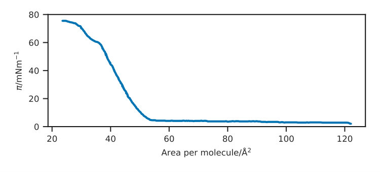 Figure 1
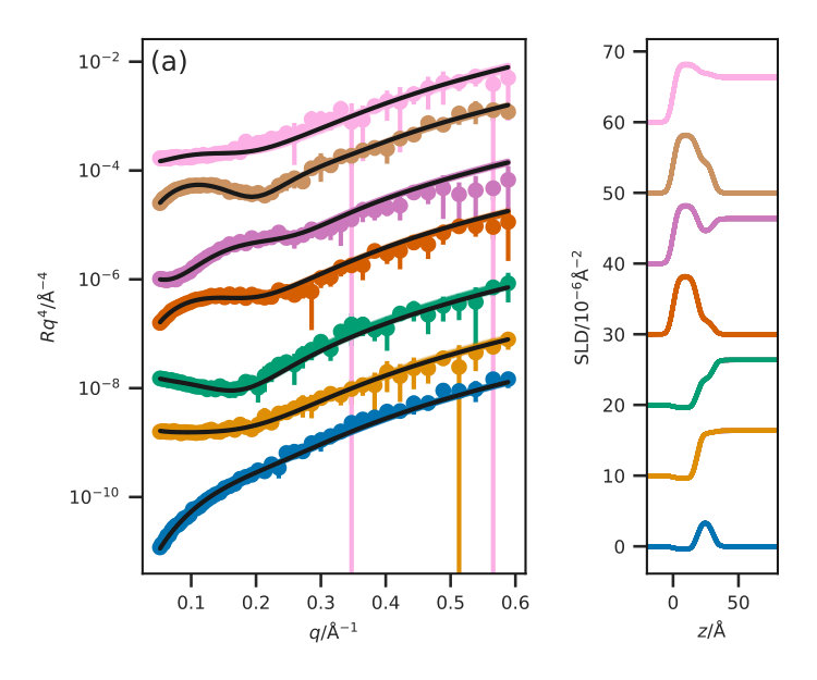 Figure 2
 Figure 3
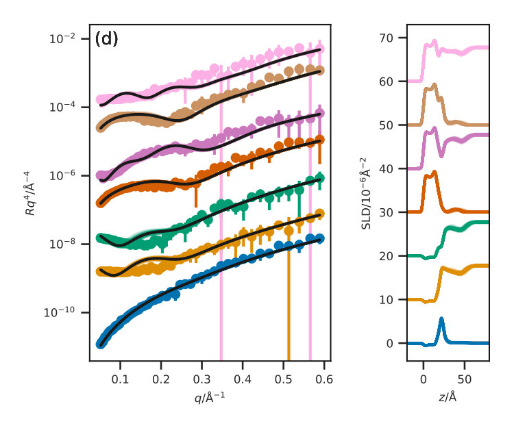 Figure 4
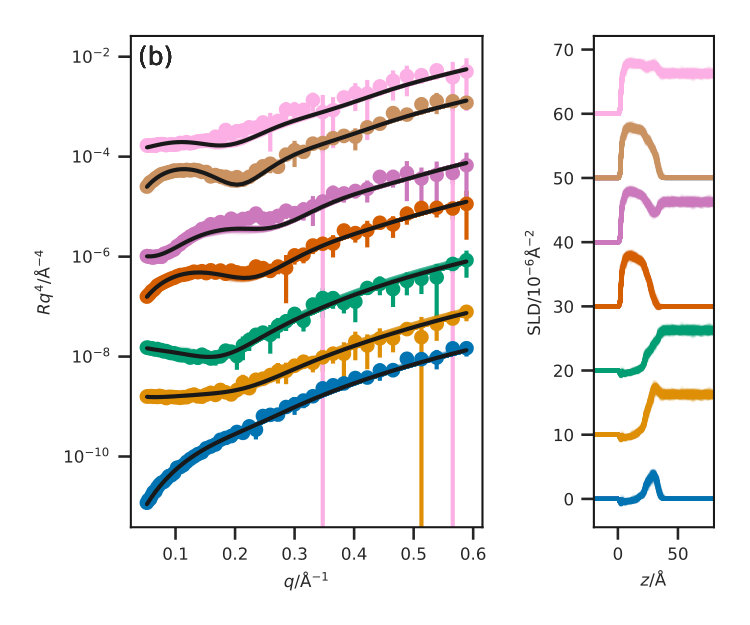 Figure 5
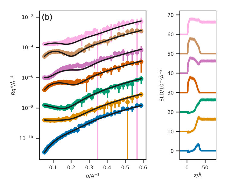 Figure 6
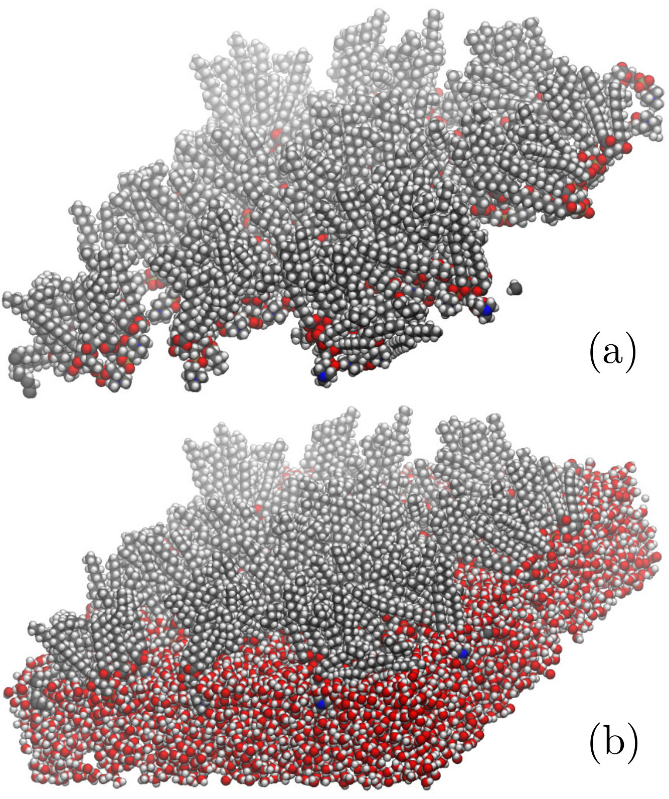 Figure 7
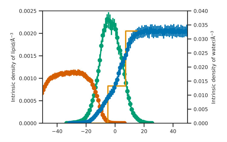 Figure 8
| Shorthand | Lipid contrast | Water contrast |
|---|---|---|
| h-\ceD2O | h-DSPC | \ceD2O |
| \ced_13-ACMW | \ced_13-DSPC | ACMW |
| \ced_13-\ceD2O | \ced_13-DSPC | \ceD2O |
| \ced_70-ACMW | \ced_70-DSPC | ACMW |
| \ced_70-\ceD2O | \ced_70-DSPC | \ceD2O |
| \ced_83-ACMW | \ced_83-DSPC | ACMW |
| \ced_83-\ceD2O | \ced_83-DSPC | \ceD2O |
| / | APM/ | xy-cell length/ |
|---|---|---|
| 20 | 47.9 | 69.1 |
| 30 | 46.4 | 68.1 |
| 40 | 45.0 | 67.1 |
| 50 | 44.6 | 66.0 |
| Contrast | Monolayer model | Slipid | Berger | MARTINI |
|---|---|---|---|---|
| h-\ceD2O |
Peer Reviews
No public reviews on file for this paper yet. If you reviewed it on a platform where reviews are public (OpenReview, ICLR, NeurIPS, ICML), you can paste yours below so the community can read it here.
Code & Models
Videos
No videos yet. Explain this paper in a talk, walkthrough, or lecture? Add one.
Assessing molecular simulation for the analysis of lipid monolayer reflectometry
A. R. McCluskey
Department of Chemistry, University of Bath, Claverton Down, Bath, BA2 7AY, UK
Diamond Light Source, Harwell Campus, Didcot, OX11 0DE, UK
J. Grant
Computing Services, University of Bath, Claverton Down, Bath, BA2 7AY, UK
A. J. Smith
Diamond Light Source, Harwell Campus, Didcot, OX11 0DE, UK
J. L. Rawle
Diamond Light Source, Harwell Campus, Didcot, OX11 0DE, UK
D. J. Barlow
Institute of Pharmaceutical Science, King’s College London, London, SE1 9NH, UK
M. J. Lawrence
Division of Pharmacy and Optometry, University of Manchester, Manchester, M13 9PT, UK
S. C. Parker
Department of Chemistry, University of Bath, Claverton Down, Bath, BA2 7AY, UK
K. J. Edler
Department of Chemistry, University of Bath, Claverton Down, Bath, BA2 7AY, UK
Abstract
Using molecular simulation to aid in the analysis of neutron reflectometry measurements is commonplace. However, reflectometry is a tool to probe large-scale structures, and therefore the use of all-atom simulation may be irrelevant. This work presents the first direct comparison between the reflectometry profiles obtained from different all-atom and coarse-grained molecular dynamics simulations. These are compared with a traditional model layer structure analysis method to determine the minimum simulation resolution required to accurately reproduce experimental data. We find that systematic limits reduce the efficacy of the MARTINI potential model, while the Berger united-atom and Slipids all-atom potential models agree similarly well with the experimental data. The model layer structure gives the best agreement, however, the higher resolution simulation-dependent methods produce an agreement that is comparable. Finally, we use the atomistic simulation to advise on possible improvements that may be offered to the model layer structures, creating a more realistic monolayer model.
Usage
Electronic Supplementary Information (ESI) available: All analysis/plotting scripts and figure files, allowing for a fully reproducible, and automated, analysis workflow for the work presented is available at https://github.com/arm61/sim_vs_trad (DOI: 10.5281/zenodo.2600729) under a CC BY-SA 4.0 license. Reduced experimental datasets are available at https://researchdata.bath.ac.uk/id/eprint/586, under a CC-BY 4.0 license.
I Introduction
Neutron and X-ray reflectometry techniques are popular in the study of layered structures, such as polyelectrolyte-surfactant mixtures Llamas et al. (2018), lipid bilayer systems Waldie et al. (2018), electrodeposited films Beebee et al. (2019), and dye-sensitised solar cell materials McCree-Grey et al. (2015). Unlike other surface-sensitive techniques, such as atomic force microscopy (AFM) or scanning electron microscopy (SEM), reflectometry methods can investigate buried interfaces in addition to the material surface. This is due to the ability of neutrons and X-rays to probe more deeply into a material than an AFM tip or the electron. Additionally, reflectometry techniques can more easily provide information about the average structure over large regions of material, resulting in significantly improved sampling, compared with microscopy techniques Renaud et al. (2009). The growth in popularity of reflectometry techniques can be attributed to the significant development of both neutron and X-ray reflectometry instrumentation, such as FIGARO, the horizontal neutron reflectometer at the ILL Campbell et al. (2011), and the beam deflection system at the I07 beamline of the Diamond Light Source Arnold et al. (2012).
Typically, the analysis of a neutron or X-ray reflectometry profile is achieved by the application of the Abelès matrix formalism for stratified media Abelès (1948); Parratt (1954) to a model layer structure. These layer structures are usually defined by the underlying chemistry of the system, for example, the chemically-consistent method that we previously used McCluskey et al. (2019a), which accounts for the chemical linkage between the phospholipid head and tail layers. However, there has been growing interest in the use of molecular dynamics simulations to inform the development of these layer structures. This is due to the fact that the equilibrium structures for soft matter interfaces, that are often of interest in reflectometry studies, are accessible on all-atom simulation timescales Scoppola and Schneck (2018). However, to the authors’ knowledge, no work has directly compared different levels of simulation coarse-graining in order to assess the required resolution for the accurate reproduction of a given neutron reflectometry profile.
The use of MD-driven analysis of neutron reflectometry usually involves, either the calculation of the SLD profile from the simulation or the full determination of the reflectometry profile. In the former case, the calculated SLD profile may be compared with the SLD profile determined from the use of a model layer structure analysis method. Bobone et al. used such a method to study the antimicrobial peptide trichogin GA-IV within a supported lipid bilayer Bobone et al. (2013). A four layer-model consisted of the hydrated \ceSiO2 layer, an inner lipid head-region, a lipid tail-region, and an outer lipid head region. The SLD profile from the MD simulations agreed well with that fitted to the reflectometry data from this model layer structure.
The reflectometry profile was calculated explicitly from classical simulation in the works of Miller et al. and Anderson and Wilson Miller et al. (2003); Anderson and Wilson (2004). In these, an amphiphilic polymer at the oil-water interface was simulated by Monte Carlo and MD respectively, and the neutron reflectometry profile found by splitting the simulation cell into a series of small layers and applying the Abelès matrix formalism. There was good agreement between the experimental and calculated reflectometry, for low interface coverages of the polymer. Another study that has made a direct comparison between the atomistic simulation-derived reflectometry and those measured experimentally is that of Darré et al. Darré et al. (2015). Darré et al., NeutronRefTools was developed to produce the neutron reflectometry profile directly from an MD simulation. The particular system studied was a supported 1,2-dimyristoyl-sn-glycero-3-phosphocholine (DMPC) lipid bilayer, again good agreement was found between the simulation-derived profile and the experimental measurement. However, the nature of the support required a correction for the head-group hydration to be imposed to achieve this agreement.
Koutsioubas used the MARTINI coarse-grained representation of a 1,2-dipalmitoyl-sn-glycero-3-phosphocholine (DPPC) lipid bilayer to compare with experimental reflectometry Koutsioubas (2016). This work showed that the parameterisation of the MARTINI water beads was extremely important in the reproduction of the reflectometry data, as the non-polarisable water bead would freeze into crystalline sheets resulting in artefacts in the reflectometry profiles calculated. The work of Hughes et al. studied again a DPPC lipid bilayer system Hughes et al. (2016), albeit an all-atom representation, that was compared with a supported DPPC lipid bilayer system measured with polarised neutron reflectometry. The SLD profile found from MD was varied to better fit the experimental measurement, resulting in good agreement. Additionally, the ability to vary the SLD profile was used to remove artefacts that arose when the MD simulations were merged with the Abelès matrix formalism. This was done to account for regions present in the experiment that were not modelled explicitly.
In all of the examples discussed so far there is no direct comparison between the reflectometry profile determined from simulation and that from the application of a traditional analysis method. Indeed, the only example, to the authors’ knowledge where a direct comparison was drawn is the work of Dabkowska et al. Dabkowska et al. (2014). This work compares the reflectometry profile from a DPPC monolayer at the air-water interface containing dimethyl sulfoxide molecules with a similar molecular dynamics simulation parameterised with the CHARMM potential model. The use of multimodal analysis allowed the determination of the position of a concentration of DMSO molecules at a particular region within a monolayer and the orientation of such molecules.
The previously mentioned work of Koutsioubas involved the use of the MARTINI coarse-grained force field to simulations the DPPC bilayer system Koutsioubas (2016). The use of atomistic simulation for soft matter systems, such as a lipid bilayer, is undesirable as this requires a huge number of atoms to be simulated, due to the large lengths scales involved. The purpose of simulation coarse-graining is to reduce the number of particles over which the forces must be integrated, additionally by removing the higher frequency bond vibrations, the simulation timestep can also be increased Pluhackova and Böckmann (2015). Together, these two factors enable an increase in both simulation size and length. The use of the MARTINI 4-to-1 coarse-grained and the Berger united-atom (where hydrogen atoms are integrated into the heavier atoms to which they are bound) potential models are particularly pertinent for application to lipid simulations as both were developed with this specific application in mind Marrink et al. (2007); Berger et al. (1997).
The MARTINI potential model involves integrating the interactions of every four heavy atoms, i.e. those larger than hydrogen, into beads of different chemical nature. This potential model attempts to simplify the interactions of lipid and protein molecules significantly by allowing for only eighteen particle types, defined by their polarity, charge, and hydrogen-bond acceptor/donor character, which are discussed in detail in the work of Marrink et al. Marrink et al. (2007). Increasing the simulation resolution gives an united-atom potential mode, where all of the hydrogen atoms are integrated into the heavier atoms to which they are bound. One of the most popular united-atom potential models for lipid simulations is that developed by Berger et al. Berger et al. (1997), with the original paper being cited 1500 times at the time of writing. Finally, the all-atom Slipid (Stockholm Lipids) lipid potential model was developed in 2012 by Jämbeck and Lyubartsev Jämbeck and Lyubartsev (2012). All three of these potential models were designed to model lipid bilayer systems.
It is clear that there is substantial interest in the use of classical simulation, and coarse-graining for the analysis of neutron reflectometry data. However, there has been no work to investigate whether the use of atomistic simulations gives more detailed than is required to reproduce the reflectometry profile accurately or to assess whether the application of a coarse-grained representation is suitable to aid in analysis. In this work, three potential models, with different degrees of coarse-graining; namely the Slipid all-atom Jämbeck and Lyubartsev (2012), Berger united-atom Berger et al. (1997), and MARTINI coarse-grained potential models Marrink et al. (2007), are compared in terms of their ability to reproduce neutron reflectometry data. We consider that this work offers a fundamental insight into the potential model resolution that is necessary to accurately reproduce experimental neutron reflectometry measurements. Furthermore, we use the highest resolution simulations to suggest possible adjustments that may be made to the model layer structure analysis methods that are typically used for the rationalisation of neutron reflectometry.
II Methodology
II.1 Neutron reflectometry measurements
The neutron reflectometry measurements analysed in this work have been previously published by Hollinshead et al. Hollinshead et al. (2009) and full details of the experimental methods can be found in this previous publication. These measurements concern the study of a monolayer of 1,2-distearoyl-sn-phosphatidylcholine (DSPC) at the air-water interface. The neutron reflectometry measurements were conducted on seven isotopic contrasts of the lipid and water. These contrasts were made up from four lipid types; fully-hydrogenated lipid (h-DSPC), head-deuterated lipid (\ced_13-DSPC), tail-deuterated lipid (\ced_70-DSPC), and fully-deutered lipid (\ced_83-DSPC), were paired with two water contrasts; fully-deuterated water \ceD2O and air-contrast matched water (ACMW), where \ceD2O and \ceH2O are mixed such that the SLD is zero. The pairing of the fully-hydrogenated lipid with ACMW was not used due to the lack of scattering available from such a system. Measurements were conducted at four different surface pressures; . Table 1 outlines the shorthands used to refer to the different contrast pairings in this work.
II.2 Molecular dynamics simulations
The DSPC monolayer simulations were made up of lipid molecules modelled with three potential models, each of a different particle grain-size. The Slipids potential model is an all-atom representation of the lipid molecules Jämbeck and Lyubartsev (2012), which was used alongside the single point charge (SPC) water model Berendsen et al. (1987), with a timestep of , the SHAKE, RATTLE, and PLINCS methods were used to constrain the \ceC-H bonds Miyamoto and Kollman (1992); Hess (2008). The Berger potential model is obtained by the integration of the hydrogen atoms into the heavy atoms to which they are bound, producing a united-atom potential model Berger et al. (1997); again the SPC water model was used. This potential model was simulated with an increased timestep of . It is noted that these timesteps are shorter than those typically used for both forcefields, and timesteps of up to have been applied previously Berger et al. (1997); Jämbeck and Lyubartsev (2012). Finally, the lowest resolution potential model used was the MARTINI Marrink et al. (2007) alongside the polarisable MARTINI water model Yesylevskyy et al. (2010), to avoid the freezing issues observed previously Koutsioubas (2016). The MARTINI 4-to-1 heavy atom beading allows for the use of a timestep. For the Slipids and Berger potential model a short-range cut-off of was used, while for the MARTINI potential model the cut-off was extended to . All simulations were conducted with temperature coupling to a heat bath at and a leap-frog integrator, and run using GROMACS 5.0.5 Berendsen et al. (1995); Lindahl et al. (2001); van der Spoel et al. (2005); Hess et al. (2008) on 32 cores of the STFC Scientific Computing resource SCARF. The simulation was of a monolayer, therefore the Ewald 3DC correction was applied to allow for the use of x/y-only periodic boundary conditions Yeh and Berkowitz (1999). A close-packed “wall” of non-interacting dummy atoms was placed at each side of the simulation cell in the z-direction to ensure that the atoms could not leave the simulation cell.
The starting simulation structure was generated using the molecular packing software Packmol Martínez et al. (2009). This was used to produce a monolayer of 100 DSPC molecules, with the head groups oriented to the bottom of the simulation cell. A layer of water was then added such that it overlapped the head groups, this was achieved using the solvate functionality in GROMACS 5.0.5. Examples of a dry and a wet monolayer can be seen in Figure 1 for the Berger potential model representation. A general protocol was then used to relax the system at the desired surface coverage, reproducing the effects of a Langmuir trough in silico. This involved subjecting the system to a semi-isotropic barostat, with a compressibility of for the Slipids and Berger simulations and for the MARTINI simulations. The pressure in the z-dimension was kept constant at , while it was increased in the x- and y-dimensions isotropically. This allowed for the surface area of the interface to reduce, as the lipid molecules have a preference to stay at the interface, while the total volume of the system stayed relatively constant, as the water molecules moved down to relax the pressure in the z-dimension. When the xy-surface area is reached that is associated with the area per molecule (APM) for each surface pressure, described by the experimental surface pressure-isotherm (Figure 2), given in Table 2, the coordinates were saved and used as the starting structure for the equilibration simulation. This equilibration simulation involved continuing the use of the semi-isotropic barostat, with the xy-area of the box fixed, allowing the system to relax at a pressure of in the z-dimension. Following the application of the pair of semi-isotropic barostats, the thickness of the water layer was typically in the region of . The equilibration period was , following which the NVT ensemble production simulations were run, on which all analyses were conducted.
II.3 Abelès matrix formalism
To compare with the simulation-derived reflectometry profiles, a modified version of the chemically-consistent surfactant monolayer model previously used in the group was applied McCluskey et al. (2019a, b). This model is implemented as a class that is compatible with the Python package refnx Nelson and Prescott (2019); Nelson et al. (2018) and is made up of two layers; the head-layer at the interface with the solvent and the tail-layer at the interface with the air. The head components have a calculated scattering length, , (found as a summation of the neutron scattering lengths of the individual atoms, see Table S1 of the ESI) and a component volume, . These make up a head-layer with a given thickness, , and interfacial roughness, , and within this layer, some volume fraction of solvent may intercalate, . The tail components also have a similarly calculated scattering length, , and component volume, . This tail-layer also has a given thickness, , and interfacial roughness, . A maximum value for the thickness of the tail-layer was imposed, this value was taken from the Tanford Equation Tanford (1980),
[TABLE]
where is the number of carbon atoms in the chain, and so for DSPC 24.3\text{,}\mathrm{\SIUnitSymbolAngstrom}$$. The SLD of the tail and head layers used in the Abelès matrix formalism can, therefore, be found as,
[TABLE]
where, is the scattering length density of the subphase (water), and indicates either the tail- or head-layer; it is assumed that the tail layer contains no solvent or air, i.e. in agreement with the work of Campbell et al. Campbell et al. (2018). To ensure that the number density of the head components and pairs of tail components is the same, the following constraint was included in the model Braun et al. (2017),
[TABLE]
A single value for the interfacial roughness was fitted for all interfaces, which was limited to be no less than , as there is only a single lipid type in each monolayer Campbell et al. (2018). Therefore, any roughness at the air-water interface is carried equally through all the layers, in a conformal fashion Kozhevnikov (2012). The modifications over the previous implementation were that the tail component volume was constrained, based on the APM (taken from the surface pressure isotherm),
[TABLE]
resulting in the monolayer model and simulation-derived models being equally constrained by the calculated surface coverage. Additionally, the head component volume was constrained to a value of , in agreement with the work of Kučerka *et al.*Kučerka et al. (2004) and Balgavý et al. Balgavý et al. (2001). A uniform background, limited to lie within of the highest -value reflected intensity, and a scale factor were then determined using refnx to offer the best agreement between the calculated reflectometry profile and that measured experimentally.
In this work, the experimental data from all seven contrasts were co-refined to a single monolayer model, where the head thickness, tail thickness, and interfacial roughness were allowed to vary. The values of the head and tail scattering lengths, along with the super and subphase SLDs are given in Table S1. For each co-refinement of seven neutron reflectometry measurements, there were in total five degrees of freedom in the fitting process, and the fitting was performed using a differential evolution algorithm, which has been shown to be particularly useful in the analysis of reflectometry data Wormington et al. (1999); Björck (2011). To obtain uncertainties on the fitted model, Markov chain Monte Carlo sampling, enabled by the emcee package Foreman-Mackey et al. (2013) was used to assess the probability distribution function for each parameter. In the MCMC sampling, 200 walkers were used over 1000 iterations, following equilibration of 200 iterations. The use of MCMC sampling allowed for Bayesian inference of the PDF for each of the variables and their respective interactions and the Shapiro test to be used to assess if each PDF was normally distributed. Parameters that were shown to be normally distributed are given with symmetric confidence intervals, while those that failed the Shapiro test are given with asymmetric confidence intervals ( confidence intervals in both cases). The Abelès matrix formalism was used to calculate the reflectometry profiles as described in the ESI.
II.4 Simulation-derived analysis
The ESI also includes a Python class that is compatible with refnx Nelson and Prescott (2019); Nelson et al. (2018) allowing for simulation-derived reflectometry profiles to be obtained, using a similar method to that employed in previous work, such as Dabkowska et al. Dabkowska et al. (2014). The Abelès matrix formalism is applied to layers, the SLD of which is drawn directly from the simulation, and the thickness of which is defined. The layer thickness used was for the Slipid and Berger potential model simulations, with an interfacial roughness between these layers is defined as . For the MARTINI potential model, a layer thickness of was used, with an interfacial roughness of , a detailed discussion for the rationale behind this is available in the ESI. Each of the production simulations were analysed with a frequency of , and the SLD profiles were determined by summing the scattering lengths, , for each of the atoms in a given layer.
[TABLE]
where, is the volume of the layer , obtained from the simulation cell parameters in the plane of the interface and the defined layer thickness. Again a uniform background, limited to lie within of the highest -value reflected intensity, and a scale factor were then determined using refnx.
II.5 Comparison between monolayer model and simulation-derived analysis
The agreement between the models from each method was assessed using the following goodness-of-fit metric, following the transformation of the data into space,
[TABLE]
where is a given -vector, which depends on the neutron wavelength and reflected angle, is the experimental reflected intensity, is the simulation-derived reflected intensity, and is the resolution function of the data.
The number of water molecules per head group, wph, was also compared between the different methods. This was obtained from the chemically-consistent model by considering the solvent fraction in the head-layer, , the volume of the head group, , and taking the volume of a single water molecule to be (from the density of water as ),
[TABLE]
The number densities, in the z-dimension, for each of the three components (lipids heads, tails, and water) may be obtained directly from the MD simulation trajectory. In order to determine the number of water molecules per headgroup from the MD simulations, a head-layer region was defined as that which contained of the lipid head number density. The ratio between the water density and the lipid head density was then found within this head-layer region.
II.6 Simulation trajectory analysis
In order to use the MD trajectory to guide the future development of the chemically-consistent layer model, it was necessary to investigate the solvent penetration into the head group region of the lipids, the roughness of each interface and the lipid tail length. The solvent penetration was determined using the intrinsic surface approach, as detailed by Allen et al. Allen et al. (2016); Pandit et al. (2003). The intrinsic surface approach enables the calculation of the solvent penetration without the effect of the monolayer roughness. This involves taking the z-dimension position of each water molecule with respect to an anchor point, in this work the anchor point was the phosphorus atom of the lipid head that was closest to the water molecule in the xy-plane. The roughness was probed by investigating the variation in positions for the start, middle, and end of each of the head and tail groups. The start of the lipid head was defined as the nitrogen atom, the middle the phosphorus and the end the tertiary carbon, while the start of the lipid tail was defined as the carbonyl carbon atom, the middle the ninth carbon in the tail and the end the final carbon atom in the tail. The distribution of each of these atom types was determined by finding the quantile for the position in the z-dimension and comparing the spread of the mean and the upper quantile. Finally, the tail length distance, was found as the distance from the carbonyl carbon atom to the final primary carbon atom of the lipid tail. All of these analyses used MDAnalysis package Gowers et al. (2016); Michaud-Agrawal et al. (2011) and the scripts that were used can be found in the ESI.
III Results & Discussion
Figure 3 presents the reflectometry and SLD profiles from each of the different methods, both the traditional layer model and the three potential model simulations, at an APM associated with a surface pressure of . This work will focus discussions on the data at this surface pressure, however other surface pressures showed similar trends and can be found in the ESI. In addition, the for each contrast, average , and standard deviation for each method are given in Table III for each contrast.
The reference list from the paper itself. Each links out to its DOI / PubMed record.
- 1Llamas et al. (2018) S. Llamas, E. Guzmán, A. Akanno, L. Fernández-Peña, F. Ortega, R. A. Campbell, R. Miller, and R. G. Rubio, J. Phys. Chem. C 122 , 4419 (2018) . · doi ↗
- 2Waldie et al. (2018) S. Waldie, T. K. Lind, K. Browning, M. Moulin, M. Haertlein, V. T. Forsyth, A. Luchini, G. A. Strohmeier, H. Pichler, S. Maric, and M. Cárdenas, Langmuir 34 , 472 (2018) . · doi ↗
- 3Beebee et al. (2019) C. Beebee, E. B. Watkins, R. M. Sapstead, V. C. Ferreira, K. S. Ryder, E. L. Smith, and A. R. Hillman, Electrochim. Acta 295 , 978 (2019) . · doi ↗
- 4Mc Cree-Grey et al. (2015) J. Mc Cree-Grey, J. M. Cole, and P. J. Evans, ACS Appl. Mater. Interfaces 7 , 16404 (2015) . · doi ↗
- 5Renaud et al. (2009) G. Renaud, R. Lazzari, and F. Leroy, Surf. Sci. Rep. 64 , 255 (2009) . · doi ↗
- 6Campbell et al. (2011) R. A. Campbell, H. P. Wacklin, I. Sutton, R. Cubitt, and G. Fragneto, Eur. Phys. J. Plus 126 , 107 (2011) . · doi ↗
- 7Arnold et al. (2012) T. Arnold, C. Nicklin, J. Rawle, J. Sutter, T. Bates, B. Nutter, G. Mc Intyre, and M. Burt, J. Synchotron Radiat. 19 , 408 (2012) . · doi ↗
- 8Abelès (1948) F. Abelès, Ann. Phys. 12 , 504 (1948) . · doi ↗
