Halo Concentrations and the New Baseline X-ray Luminosity-Temperature and Mass Relations of Galaxy Clusters
Yutaka Fujita, Han Aung

TL;DR
This paper revises the baseline X-ray luminosity-temperature and mass relations of galaxy clusters by incorporating the effects of halo concentration, predicting shallower slopes than traditional models, and confirms these predictions with simulations.
Contribution
It introduces new baseline relations for galaxy cluster X-ray luminosity and mass that account for halo concentration effects, challenging previous predictions.
Findings
Predicted $L_X$-$T_X$ relation slope is ~1.7, shallower than 2.
Numerical simulations find $L_X$-$T_X$ slope around 1.6.
Baseline $L_X$-$M_\Delta$ relation slope is ~1.1-1.2, less than 4/3.
Abstract
The standard self-similar model of galaxy cluster formation predicts that the X-ray luminosity-temperature (-) relation of galaxy clusters should have been in absence of the baryonic physics, such as radiative cooling and feedback from stars and black holes. However, this baseline relation is predicted without considering the fact that the halo concentration and the characteristic density of clusters increases as their mass decreases, which is a consequence of hierarchical structure formation of the universe. Here, we show that the actual baseline relation should be , where , instead of , given the mass dependence of the concentration and the fundamental plane relation of galaxy clusters. Numerical simulations show that , which is consistent with the prediction. We also show that the baseline…
Click any figure to enlarge with its caption.
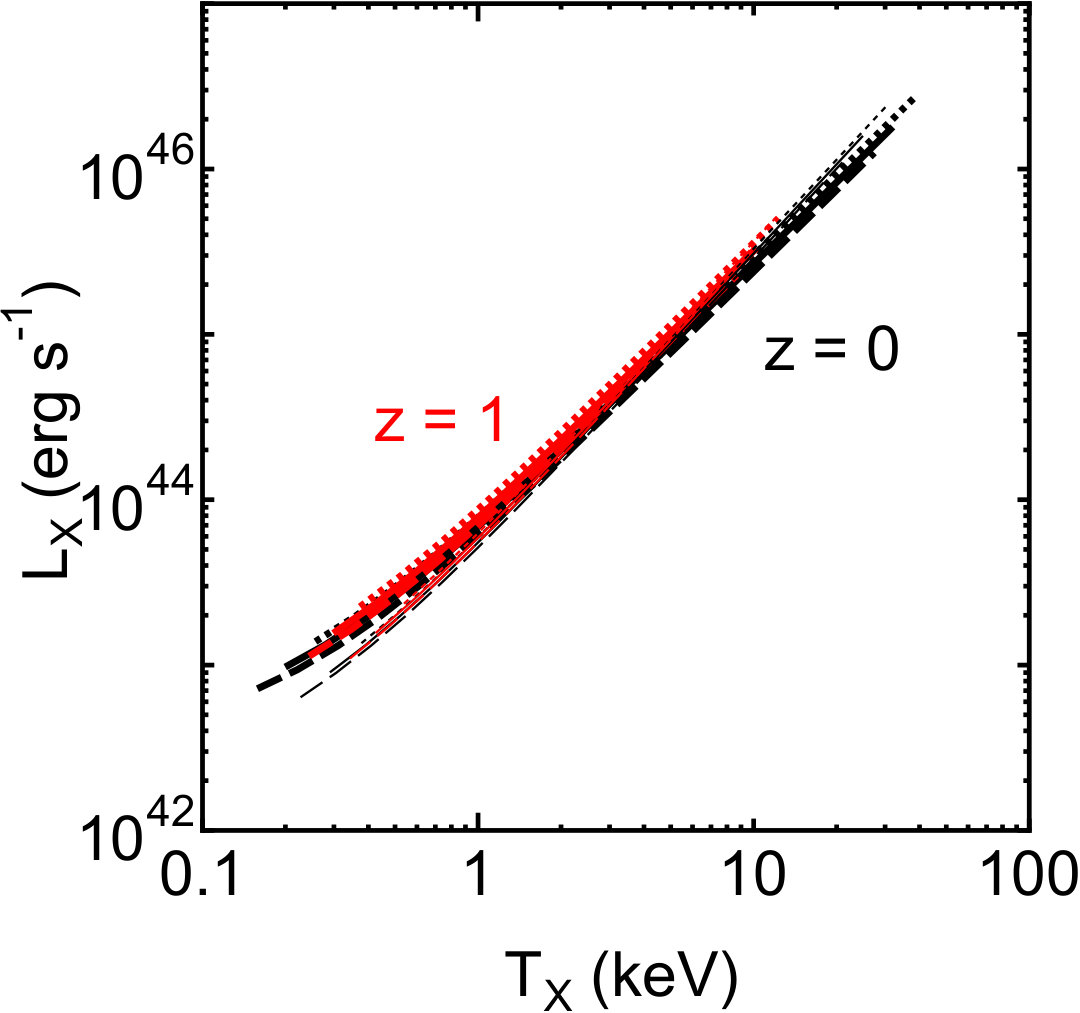 Figure 1
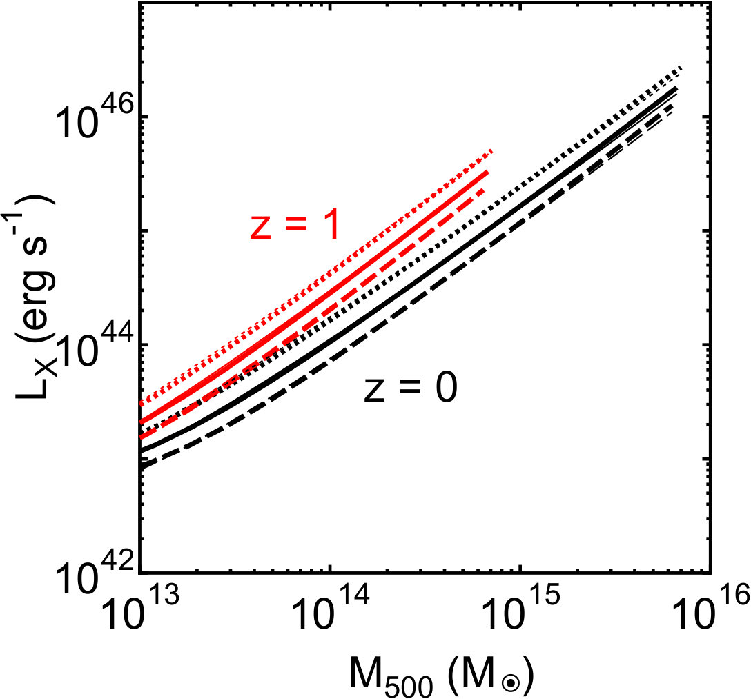 Figure 2
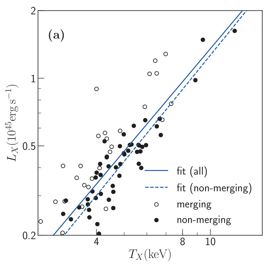 Figure 3
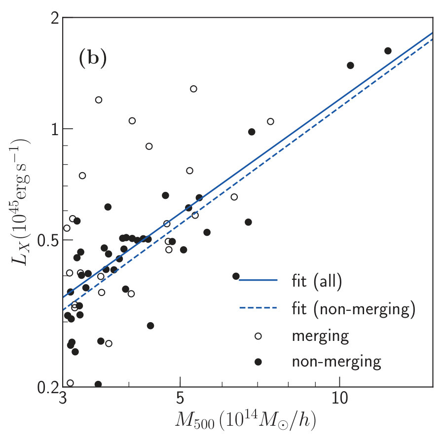 Figure 4
| -2 | 1.59–1.61 | 1.17–1.24 | 1.19–1.26 |
| -2.5 | 1.74–1.77 | 1.12–1.20 | 1.14–1.22 |
Peer Reviews
No public reviews on file for this paper yet. If you reviewed it on a platform where reviews are public (OpenReview, ICLR, NeurIPS, ICML), you can paste yours below so the community can read it here.
Videos
No videos yet. Explain this paper in a talk, walkthrough, or lecture? Add one.
Halo Concentrations and the New Baseline X-ray Luminosity-Temperature and Mass Relations of Galaxy Clusters
Yutaka Fujita11affiliationmark: , Han Aung22affiliationmark:
1Department of Earth and Space Science, Graduate School of Science, Osaka University, Toyonaka, Osaka 560-0043, Japan
2Department of Physics, Yale University, New Haven, CT 06520, USA
(Received January 1, 0000; Revised January 1, 0000)
Abstract
The standard self-similar model of galaxy cluster formation predicts that the X-ray luminosity–temperature (–) relation of galaxy clusters should have been in absence of the baryonic physics, such as radiative cooling and feedback from stars and black holes. However, this baseline relation is predicted without considering the fact that the halo concentration and the characteristic density of clusters increases as their mass decreases, which is a consequence of hierarchical structure formation of the universe. Here, we show that the actual baseline relation should be , where , instead of , given the mass dependence of the concentration and the fundamental plane relation of galaxy clusters. Numerical simulations show that , which is consistent with the prediction. We also show that the baseline luminosity–mass (–) relation should have been , where –1.2, in contrast with the conventional prediction (). In addition, some of the scatter in the – relation can be attributed to the scatter in the concentration–mass (–) relation. The confirmation of the shallow slope could be a proof of hierarchical clustering. As an example, we show that the new baseline relations could be checked by studying the temperature or mass dependence of gas mass fraction of clusters. Moreover, the highest-temperature clusters would follow the shallow baseline relations if the influences of cool cores and cluster mergers are properly removed.
Subject headings:
galaxies: clusters: general — galaxies: clusters: intracluster medium — cosmology: observations — X-rays: galaxies: cluster
1. Introduction
Clusters of galaxies have grown from slightly overdense regions of the universe. The initial density fluctuations of the universe are described by a random Gaussian field with a power spectrum having a smoothly changing power-law index. Thus, clusters are expected to have a high degree of self-similarity in scale and time, which leads to various scaling relations among observables, although the relations may be affected by the mass assembly histories of dark matter halos. The relation between the X-ray luminosity and temperature of clusters has been studied for many years, probably because it is relatively easy to measure them. Observations have shown that the relation is approximately described as (e.g. Edge & Stewart, 1991; Markevitch, 1998). This relation is thought to be influenced by feedback from active galactic nuclei (AGNs) and supernovae in galaxies in clusters (e.g. Voit et al., 2002; Borgani et al., 2004; Puchwein et al., 2008). The relation when there was no feedback is often expected to be (Kaiser, 1986; Bryan & Norman, 1998). We refer to scaling relations when there were no nongravitational effects (e.g. feedback and radiative cooling) as the “baseline relations,” because they are used as baselines when the nongravitational effects are estimated.
The conventional baseline relation of is derived assuming that cluster structure is self-similar and the characteristic density of clusters is proportional to the density of the background universe. This means that clusters at a given redshift have a common characteristic density. However, this assumption seems to be at odds with recent studies on structure formation of the universe. Numerical simulations have shown that the dark matter density profile of galaxy clusters is well represented by the Navarro–Frenk–White (NFW) density profile (Navarro et al., 1997), and that less massive clusters tend to be more concentrated and have higher characteristic densities. In other words, the characteristic density differs among clusters even at a given redshift. This is because in the standard CDM cosmology, less massive clusters form earlier and their characteristic density reflects the higher background density of the universe at their formation time (e.g. Navarro et al., 1997; Wechsler et al., 2002; Zhang et al., 2008; Ludlow et al., 2013). Thus, their mass dependence is a consequence of hierarchical structure formation of the universe (e.g. Duffy et al., 2008; Bhattacharya et al., 2013; Meneghetti et al., 2014).
Scaling relations for clusters are not necessarily limited to one-to-one correlations. For example, relations among three parameters are often considered and “fundamental planes” are the representative ones (Schaeffer et al., 1993; Adami et al., 1998; Fujita & Takahara, 1999; Verde et al., 2002; Lanzoni et al., 2004; Ota et al., 2006; Araya-Melo et al., 2009; Ettori, 2013; Maughan, 2014; Ettori, 2015). Recently, Fujita et al. (2018a, see for a review) found that observed clusters are distributed on a plane in the space of , where and are the characteristic radius and mass for the NFW profile, respectively, and is the X-ray temperature. Numerical simulations have confirmed the plane and have shown that clusters evolve along the plane. Thus, this fundamental plane reflects the structure and evolution of dark matter halos of clusters. The nongravitational effects and cluster mergers have little effect on the plane. The properties of the plane can be explained by an analytical model of structure formation constructed by Bertschinger (1985). In particular, the angle of the plane in the space of indicates that clusters have not perfectly achieved virial equilibrium because of continuous matter accretion from the surroundings (Fujita et al., 2018a). We note that the deviation from the virial equilibrium is not considered when the conventional relation is constructed.
In this study, we revise the baseline – relation considering the mass dependence of the halo concentrations and the fundamental plane. We also study the baseline luminosity–mass (–) relation as a corollary. The paper is organized as follows. In Section 2, we review the derivation of the conventional baseline relations. In Section 3, we derive the revised baseline – and – relations by taking into account the mass dependence of halo concentrations and the fundamental plane relation, and show that they deviate from the conventional relations. In Section 4, we test the predictions of our new model using the Omega500 hydrodynamical cosmological simulations of galaxy cluster formation. In Section 5, we discuss future observations of the – and – relations. In Section 6, we summarize our main results.
In this paper, we assume a spatially flat CDM cosmology with , , and the Hubble constant of km s*-1* Mpc*-1* for , unless otherwise mentioned.
2. conventional baseline relations
The conventional scaling relations are based on a gravitational collapse model of a homogeneous spherical overdense region in the Einstein-de Sitter universe (Kaiser, 1986). This region initially expands with the Hubble expansion. Then, owing to the gravity, it deviates from the expansion, and starts to collapse. The evolution is self-similar and can be treated analytically (e.g. Peebles, 1980). If the collapsed region is virialized, the average density is times the critical density of the universe. Subsequent matter accretion from the surroundings is not considered in this model.
The conventional baseline relation of can be derived as follows. First, we assume that the typical density of clusters is , where is a constant and is the critical density of the universe at redshift . The critical density depends on as in , where the Hubble parameter at is represented by and is the Hubble constant. The density does not depend on clusters and is constant at a given redshift. The corresponding cluster radius is defined as the one inside which the average density is , and the mass is written as
[TABLE]
For the overdensity, is often used because it is close to . However, it is generally difficult to observe cluster properties out to ; is also often used.
Assuming that the cooling function of the intracluster medium (ICM) is described by bremsstrahlung, the bolometric emissivity is proportional to , where is the typical density of the ICM. Here, we assume that . Since the typical volume of a cluster is proportional to , the X-ray luminosity of clusters is represented by
[TABLE]
If we assume the virial equilibrium, the X-ray temperature is given by using equation (1). Considering that and , we finally obtain the relation of
[TABLE]
from equation (2) (Kaiser, 1986; Bryan & Norman, 1998). Thus, for a given . Similarly, the baseline luminosity–mass relation can be obtained as in (Bryan & Norman, 1998).
3. New baseline relations
However, the above derivations do not take into account the mass profile of clusters. Numerical simulations have shown that the dark matter density profile of galaxy clusters is well represented by the NFW density profile (Navarro et al., 1997):
[TABLE]
where is the cluster centric radius, is the characteristic radius, and is the normalization. The radius is smaller than for clusters if and 500. We define the characteristic mass as the mass enclosed within , and define the characteristic density as . The halo concentration parameter is given by
[TABLE]
The mass profile of the NFW profile is then given by
[TABLE]
From this equation, the characteristic mass can be expressed in terms of and :
[TABLE]
-body simulations have shown that is a decreasing function of for a given , with a considerable dispersion ( dex) due to the diversity in cluster ages for a given mass (e.g. Duffy et al., 2008; Bhattacharya et al., 2013; Meneghetti et al., 2014; Fujita et al., 2018b). While a wide mass range of halos have concentration of at high redshifts, only most massive halos have and others have higher concentration at (Child et al., 2018). As a result, from equations (1) and (5), the scale radius and the characteristic density also depend on and .
Since the emissivity of the ICM is proportional to the density squared, the X-ray luminosity of clusters should reflect the structure of their central region where the density is high. If we assume that the dark matter profile follows the NFW profile (equation (4)) and that the ICM density follows that of dark matter (), the characteristic volume of a cluster should be and the X-ray luminosity is
[TABLE]
in contrast with equation (2). Since depends on and while is constant for a given , this fact differentiates equation (8) from equation (2). In other words, the variation of the halo concentration among clusters is not considered in the derivation of equation (3). As clusters with larger tend to have larger , we expect that the mass dependence of affects the – relation as well as the – relation if they are derived from equation (8) (see also Enoki et al., 2001).
The revised baseline – and – relations of clusters can be obtained using the mass dependence of the concentration parameter and the fundamental plane relation given by
[TABLE]
where is a representative point on the fundamental plane (Fujita et al., 2018a, b).111We use kpc, , and keV based on the results of the MUSIC simulations (Meneghetti et al., 2014; Fujita et al., 2018a). Note that is the core excised temperature. The relation does not depend on at least and indicates that clusters in general have not achieved virial equilibrium (Fujita et al., 2018a). The equation (9) can be derived from the entropy constant given in the similarity solution by Bertschinger (1985); the constant reflects the conservation of the ICM entropy. The relation depends on the spectral index of the density perturbations of the universe, because the overdense region that later becomes the inner part of a cluster and gives the inner boundary of the solution of Bertschinger (1985) evolves from the density perturbations (Fujita et al., 2018a). Although the index should be at cluster scales (e.g. Eisenstein & Hu, 1998; Diemer & Kravtsov, 2015), we treat simply as a parameter here. We assume and , both of which are consistent with observed and simulated fundamental planes (Fujita et al., 2018b). Since equation (9) shows that is a function of and , it is also a function of and .
Although we considered only bremsstrahlung for the cooling function () in Section 2 and in equation (8) for simplicity and illustration, we will now include the effect of metal-line cooling, which introduces additional dependence on the ICM metallicity . The X-ray luminosity would then be given by , where and we adopt the following metallicity-dependent cooling function given by
[TABLE]
(Fujita & Ohira, 2013), which approximates the cooling function derived by Sutherland & Dopita (1993) for K and .
Now, using as a parameter, we can draw the – relation (Figure 1). We assume that . Assuming that the ICM consists of hydrogen and helium222The inclusion of metals have little influence (only a few percent change in ) as long as ., the electron density is given by , where is the proton mass and is the gas mass fraction of massive clusters (e.g. Biviano & Salucci, 2006; Gonzalez et al., 2013; Dvorkin & Rephaeli, 2015). The solid lines are the fiducial relations that are calculated using the analytic function333https://bitbucket.org/astroduff/commah of obtained by Correa et al. (2015).
Considering the dispersion of the – relation, we also represent the – relations when (fiducial) is replaced by (dotted line) or (dashed line). Figure 1 shows that the solid, dotted, and dashed lines are almost identical, which means that the dispersion of the – relation does not introduce a scatter in the – relation. Moreover, the – relation does not depend sensitively on redshift, which is in contrast to the relation derived based on the simple self-similar model on a scale of (equation (3)). Since the baseline relation does not evolve (Figure 1), observed evolution, if any, can be attributed to additional baryonic physics, such as gas cooling and feedback.
Observationally, there seems to be no consensus about the redshift evolution of the – relation so far (e.g. Böhringer et al., 2012), although Reichert et al. (2011) concluded that the evolution of X-ray luminosity for a given temperature is slower than predicted by a simple self-similar model (see equation 3). Note that the – relation in Figure 1 is constructed from and , which reflect cluster properties on a scale of . The observed – relation has a larger scatter ( dex; e.g. Maughan et al. 2012) than those shown by the dotted and dashed lines in Figure 1, which suggests that actual X-ray luminosities are impacted by local and/or temporary phenomena around the cluster centers (e.g., AGN feedback in cool cores and/or disruption of the cores by cluster mergers) and that the effects differ among clusters.
Table 1 summarizes the values of the index of the – relation () for different and a temperature range of keV. For each index, the smaller one is for and the larger one is for . The index is determined for the fiducial relation (solid lines in Figure 1) but the results are almost unchanged even if we take the dotted or dashed lines. Although the slope of the – relation becomes slightly shallower for keV due to the metal-line cooling (Figure 1), the magnitude of this effect is quite small. The indices for a temperature range of keV is larger than those for keV only by . We, therefore, conclude that the index should be smaller than two and should be –1.8 if the ICM density profile follows the dark matter profile. The shallower slope is ascribed to the increase in the halo concentration and the characteristic density for lower temperature (less massive) clusters. We expect that the smaller index is realized when additional physics such as feedback, radiative cooling, and disturbance by cluster mergers are ignorable, because the ICM settled in the potential well of the dark matter halo and is the only spatial scale of the NFW profile.
It may be instructive to represent the – relation only by the fundamental plane. From equations (8), (9), and , we obtain , which is for , and for . This means that the – relation is not sensitive to and that the – relation is close to an “edge-on view” of the fundamental plane (see also Fujita & Takahara 1999). Thus, the relation is almost independent of and has almost no dispersion (Figure 1(a)), even though is a function of and .444The fundamental plane reflects the higher concentration of lower-mass and/or higher-redshift clusters. The function approximately defines the evolution track of clusters on the fundamental plane (Figure 2 in Fujita et al. 2018b).
As is a function of and , the – relation can immediately be obtained. Figure 2 shows the – relation for . Table 1 reports the index of the relation () for a temperature range of keV, where and are for and 500, respectively. For each index, the smallest one is for and the largest one is for . The indices are determined for the fiducial relations, indicated with the solid lines in Figure 2. The indices for a temperature range of keV is larger than those for keV only by . The table shows that , which is slightly smaller than the prediction of the conventional self-similar model (; Section 2). Clusters with host a plasma with an X-ray emission with a relatively larger contribution from metal-line recombination. For a given mass, at is larger than that at , mainly because the characteristic density is larger for the former. In contrast to the – relation, the dispersion of the – relation scatters the – relation (dotted and dashed lines in Figure 2), which indicates that the – relation is not an edge-on view of the fundamental plane. Moreover, as is the case of the – relation, the – relation is written as when only the fundamental plane relation is used. Since is approximately represented by (equation (7)), the luminosity is given by for , and for . This means that the – relation is sensitive to and is scattered by the variety.
We note that observationally determined directions of the fundamental plane have some uncertainties caused by observational errors (see the contours in Figure 2 of Fujita et al., 2018a). On the other hand, numerical simulations have shown that the plane is intrinsically thin ( dex; Fujita et al. 2018a) and that the thickness of the plane does not affect the plane normal. However, the plane relation determined by the simulation results has a small deviation from the relation we assumed in equation (9) (see the marks in Figure 2 of Fujita et al., 2018a). They seem to be associated with treatment of cool cores and presence or absence of nongravitational effects. In order to estimate the influence of the deviation, we construct fundamental plane relations for each of the simulation sets (MUSIC, NF0, FB0, and FB1 in Fujita et al., 2018a) instead of equation (9) and derive the indices for the – and the – relations. We found that and . These uncertainties motivate us to directly simulate the – and – relations in the next section.
4. Numerical simulations
In order to confirm the predictions made in the previous section, we analyze the results of the nonradiative version of the Omega500 hydrodynamical cosmological simulations (Nelson et al., 2014). We do not include radiative cooling and feedback by AGNs and supernovae when we calculate gas dynamics because the purpose of this study is to find the baseline – and – relations.
The simulation Omega500 is run with Adaptive Tree Refinement, an Eulerian code that uses adaptive refinement in space and time (Kravtsov, 1999; Kravtsov et al., 2002; Rudd et al., 2008). The softening length is kpc for both dark matter particles and gas cells in the high-resolution regions. Nonadaptive refinement in mass necessary for resolving cores of the clusters is employed so that the highest mass resolution for the dark matter particles is . The simulation box has a comoving box length of Mpc. We select all of the 65 clusters at with regardless of dynamical state. We compute the emission-weighted temperature including the core. We kept the core because these simulations are nonradiative and thus do not present cool-core features. The bolometric luminosity and the temperature are derived within a radius . This choice of the radius does not affect the results much if the radius is large enough. This is because X-ray emissivity is proportional to density squared and most of the X-ray emission comes from the central region of clusters. The metal abundance is assumed to be in the calculation of the luminosity .
In Figure 3, we show the results for the whole sample (filled open circles). In Figure 3(a), we fit the data in log space with the function using BCES orthogonal regression (solid line; Akritas & Bershady, 1996). The index for the fit is (all uncertainties are quoted at the 1 confidence level unless otherwise mentioned), which is almost consistent with the prediction for in Section 3 (Table 1). However, some of the clusters in Figure 3 are merging clusters, for which the ICM profiles are often significantly deviated from the dark matter profiles. Thus, we study the – relation excluding merging clusters. We define merging clusters as those that undergo a merger of mass ratio of at least one-sixth in the past 2 Gyr, which is about a typical relaxation time scale. Figure 3(a) shows that the dispersion of the – relation is reduced if we choose only nonmerging clusters. The result of a fit for the nonmerging clusters is indicated by the dashed line and the index is . Changing the merger mass ratio limit to one-fifth or one-seventh only shifts the slope within . Again, the index is consistent with the prediction when (Table 1), and is clearly rejected. For the – relation (Figure 3(b)), the results of fits show for the whole sample and for the nonmerging clusters. Compared with the – relation (Figure 3(a)), the dispersion is larger, which may be related to the dispersion of the – relation (Figure 2). The value of is consistent with the predictions for in Table 1 and is clearly rejected.
5. Discussion
We have shown that the suggested new relations for – and – once a mass profile is properly taken into account are shallower than the ones predicted from a self-similar model. With the improved understanding of the luminosity-mass relation, we may explore new methods of mass measurements through X-ray luminosity. As shown in Figure 2, a typical scatter of 0.1 dex in the – relation can produce a scatter of approximately 0.15 dex in the – relation. This will account for more than 50% of scatter in observed scatter (e.g. Maughan, 2007; Rykoff et al., 2008; Zhang et al., 2008, but see Andreon et al., 2016). This suggests that that the scatter caused by hierarchical structure formation can be comparable to nongravitational effects, and proper modeling of this effect of halo concentrations on the – relation will help reduce the scatter and potentially open the path for mass measurements through X-ray luminosity.
If the shallow slopes of the baseline relations are observed, it will be a proof of the hierarchical structure formation. However, real clusters are affected by the aforementioned additional nongravitational effects. For example, the gas fraction of the central region of observed clusters () is generally smaller than the baryon fraction of the universe (e.g. Vikhlinin et al., 2006; Sun et al., 2009). This is mostly explained as a result of the feedback from AGNs and supernovae, although some of the baryon in clusters is consumed in star formation. The feedback leads to an increase in and from the baseline relations. Observations have shown that –3.7 and –2.0 (e.g. Edge & Stewart, 1991; Ebeling et al., 1996; Markevitch, 1998; Arnaud & Evrard, 1999; Ikebe et al., 2002; Reiprich & Böhringer, 2002; Ettori et al., 2004; Hicks et al., 2008; Zhang et al., 2008; Pratt et al., 2009; Reichert et al., 2011). Some of the studies have shown that even if cluster cores are excised in the analysis, the slopes (e.g. and ; Maughan 2007) are steeper than those of the baseline relations ( and –1.2). This means that the feedback impacts on the ICM density beyond the cores. If we assume that the indices of the observed relations are and and those of the baseline relations are and , the gas mass fraction at should have a temperature and mass dependence of and , respectively. This is because the typical X-ray emissivity depends on the gas fraction as . The dependences are steeper than those expected in the simple self-similar model ( and for ; see Böhringer et al., 2012). It may be easier to confirm the – relation than the – relation because the former is steeper. If these dependences are observationally confirmed, they may indirectly prove the shallow baseline relations and hierarchical structure formation.
The steeper slopes of the – and – relations, when the new baseline relations are adopted, can be explained as follows. The new baseline relations reflect that low-temperature clusters have higher concentrations than high-temperature clusters. Thus, the low-temperature clusters have denser gas in the central region compared with those when they have the same concentration as the high-temperature clusters. Thus, stronger feedback and smaller are required for the low-temperature clusters in order to reproduce the observed steep – and – relations. In the Appendix, we performed a mock analysis of the – relation and showed that a sample of clusters is enough to discriminate from . This method to confirm the hierarchical structure formation may be easier than observationally determining the slope of the – relation because the latter is affected by a large scatter (e.g. Okabe & Smith, 2016).
We note that sample selection could be more important than the number of clusters. For example, the observed – and – relations could be affected by cluster mergers as well as cool cores. In fact, Maughan et al. (2012) derived a rather small index is of for nonmerging clusters with keV when the emission from the cool cores are excised, although a similar analysis done by Mahdavi et al. (2013) showed that .555Previous studies that excise cool cores often define the core as the region within , where is the constant (e.g. and ; Maughan et al. 2012; Mahdavi et al. 2013). If the characteristic density of clusters is rather than , the definition of the cool core should also be based on . This redefinition could change the slopes of the observed – and – relations, although this is out of the scope of this study. If the former is the case, it has already suggested the shallower slope of the – relation (), although cannot be rejected. Since the gas fraction comes close to the universal value for the highest-temperature clusters (e.g. Vikhlinin et al., 2006), the feedback appears to be less effective for them and the shallower slope is more likely to be realized. Thus, through the – relation for highest-temperature clusters, the hierarchical structure formation could be proved without studying the – relation. In the near future, eROSITA would detect enough numbers of massive or higher-temperature clusters and would enable us to confirm the shallow – and – relations with a sufficient degree of accuracy. Follow-up observations with Chandra and XMM-Newton are also important.
The baseline relations we found should be taken into account especially when the feedback effects are estimated based on the – and/or – relations. For example, our discovery indicates that even if the observed index is proven to be or after considering the effects of cluster mergers and cool cores, it does not mean that those clusters are free from feedback because it is still larger than that for the baseline relation ( or –).
6. Summary
Using the mass dependence of halo concentrations and the fundamental plane relation of galaxy clusters, we have shown that the index of the baseline – relation of clusters, that is, the one when additional physics such as feedback, radiative cooling, and disturbance by cluster mergers are ignored, should be –1.8. The value is smaller than , which was previously estimated based on a simple self-similar model. For the baseline – relation, we showed that the index should be –1.2, which is also smaller than the prediction () of the self-similar model. These are because the halo concentration and the characteristic density of clusters increase as the cluster mass decreases in the hierarchical structure formation in a CDM universe. This mass dependence was not considered when the conventional relations of and were derived. The new baseline relations would be useful when the feedback effects are estimated based on scaling relations. The baseline relations could be checked by the temperature or mass dependence of gas mass fraction of clusters. We also indicated that the highest-temperature clusters may follow relations close to the new baseline relations if the influences of cool cores and cluster mergers are appropriately treated. This is because the feedback effects are expected to be minimum for those clusters. Near-future cluster surveys (e.g. eROSITA) may enable us to confirm the relations more precisely. If they are actually confirmed, it would be a proof of the hierarchical structure formation.
We thank the anonymous referee, whose comments improved the clarity of this paper. We also thank Hans Böhringer and Daisuke Nagai for useful comments and discussion. This work was supported by MEXT KAKENHI No. 18K03647 (Y.F.).
Appendix A Mock analysis of the gas fraction–temperature relation
For a quantitative discussion, we perform a simple mock analysis of the – relation. We create a mock sample of clusters in a temperature range of . Since the number of clusters with larger temperatures is smaller, we set the temperatures of the clusters following the equation of , where is a random number between zero and one, and we assume that keV and keV. As a result, the expected number of clusters between 10 and 12 keV is about one-forth of that between 4 and 6 keV. The expected gas fraction at , where is an appropriate constant, is assumed to be
[TABLE]
where is the fraction for clusters with keV, and we assume . The predicted indices for the new and the conventional relations are and , respectively (Section 5). For the conventional relation, we implicitly assume that the halo concentration is independent of the temperature and . Clusters distribute along the relation (A1) with an intrinsic scatter. For the gas fraction at or , observations have shown that the intrinsic scatter is 10% and observational uncertainties are much smaller than the intrinsic scatter (e.g. Vikhlinin et al., 2006). As far as we know, there are no previous observational studies on the gas fractions at . The determination of is rather difficult and the observational uncertainties may be % (e.g. Ettori et al., 2010). Fortunately, the gas fraction is not sensitive to the radius, and even the 30% uncertainties of the radius cause % uncertainties for the gas fraction of relaxed clusters (e.g. Figure 6 of Landry et al., 2013). Thus, in addition to the 10% intrinsic scatter, which is given by a random gaussian, we introduce 10% observational uncertainties for . We also assume 3% observational uncertainties for .
For a given index , we generate a total of realizations of the sample. Using BCES regression (Akritas & Bershady, 1996), we fit the data with equation (A1) assuming that and are free parameters, and derive the uncertainties of . The results are almost the same if we adopt a BCES orthogonal regression. If we assume that and (the new baseline prediction), the result of the realizations is . This means that (the conventional baseline prediction) can be rejected with a sample of clusters. We note that for . On the other hand, if we assume that and , the result of the realizations is .
The above estimations suggest that the new baseline relation can be confirmed once at are derived for not too many clusters. The radius can be determined by fitting an observed mass profile with equation (6). Alternatively, if at two different are obtained (say and 2500), can also be derived from equations (1), (5), and (6).
The reference list from the paper itself. Each links out to its DOI / PubMed record.
- 1Adami et al. (1998) Adami, C., Mazure, A., Biviano, A., Katgert, P., & Rhee, G. 1998, A&A, 331, 493
- 2Akritas & Bershady (1996) Akritas, M. G., & Bershady, M. A. 1996, Ap J, 470, 706
- 3Andreon et al. (2016) Andreon, S., Serra, A. L., Moretti, A., & Trinchieri, G. 2016, A&A, 585, A 147
- 4Araya-Melo et al. (2009) Araya-Melo, P. A., van de Weygaert, R., & Jones, B. J. T. 2009, MNRAS, 400, 1317
- 5Arnaud & Evrard (1999) Arnaud, M., & Evrard, A. E. 1999, MNRAS, 305, 631
- 6Bertschinger (1985) Bertschinger, E. 1985, Ap JS, 58, 39
- 7Bhattacharya et al. (2013) Bhattacharya, S., Habib, S., Heitmann, K., & Vikhlinin, A. 2013, Ap J, 766, 32
- 8Biviano & Salucci (2006) Biviano, A., & Salucci, P. 2006, A&A, 452, 75