Electron and Proton Heating in Transrelativistic Guide Field Reconnection
Michael E. Rowan (1), Lorenzo Sironi (2), Ramesh Narayan (1) ((1), Harvard, (2) Columbia)

TL;DR
This study uses 2D particle-in-cell simulations to investigate how magnetic reconnection in transrelativistic plasmas heats electrons and protons, revealing the influence of guide field strength and plasma beta on energy partitioning.
Contribution
It provides new insights into the dependence of electron and proton heating on guide field and plasma conditions in transrelativistic reconnection, relevant for accretion flows around black holes.
Findings
Electrons receive up to 93% of heating with strong guide fields at low beta.
Protons are less heated as guide field increases, especially at low beta.
At high beta (~2), electrons and protons share heating equally (~50%).
Abstract
The plasma in low-luminosity accretion flows, such as the one around the black hole at the center of M87 or Sgr A* at our Galactic Center, is expected to be collisioness and two-temperature, with protons hotter than electrons. Here, particle heating is expected to be controlled by magnetic reconnection in the transrelativistic regime -, where the magnetization is the ratio of magnetic energy density to plasma enthalpy density. By means of large-scale 2D particle-in-cell simulations, we explore for a fiducial how the dissipated magnetic energy gets partitioned between electrons and protons, as a function of (the ratio of proton thermal pressure to magnetic pressure) and of the strength of a guide field perpendicular to the reversing field . At low , we find that the fraction…
Click any figure to enlarge with its caption.
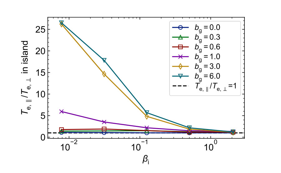 Figure 1
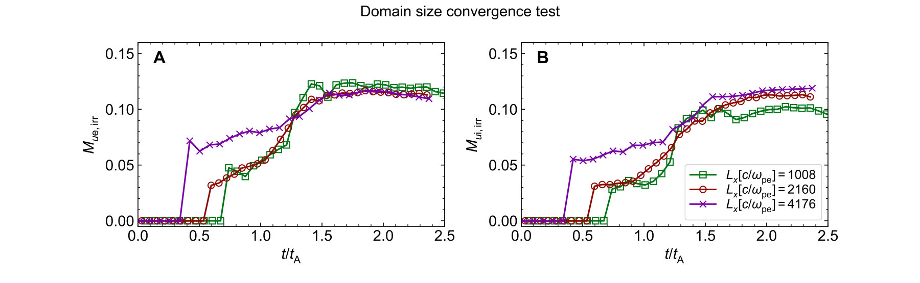 Figure 2
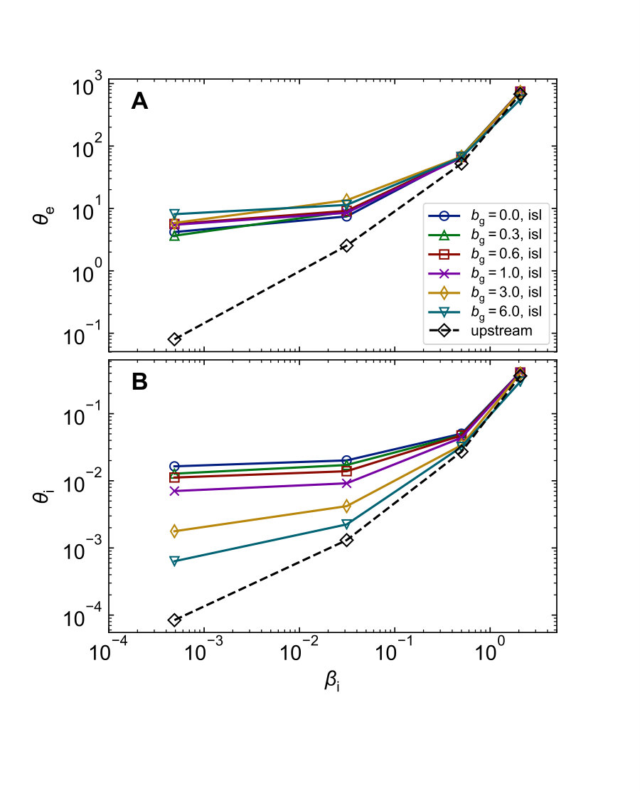 Figure 3
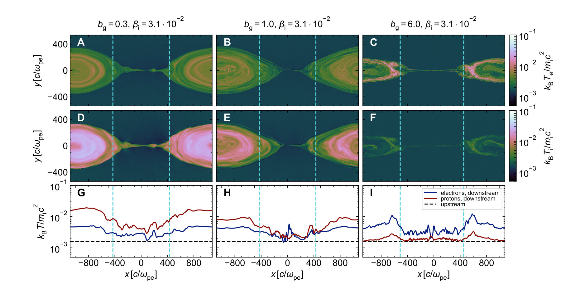 Figure 4
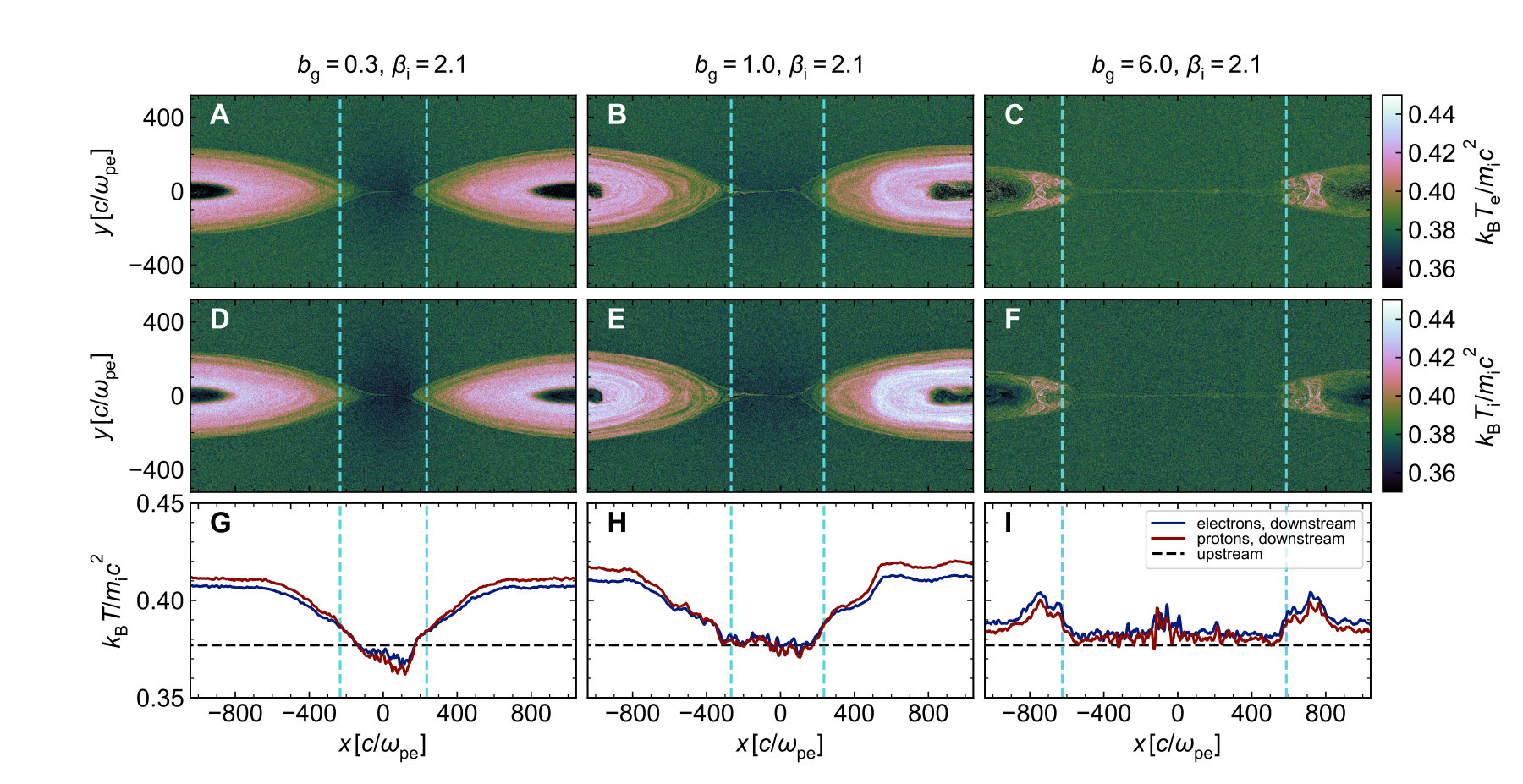 Figure 5
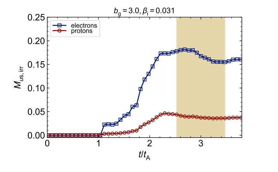 Figure 6
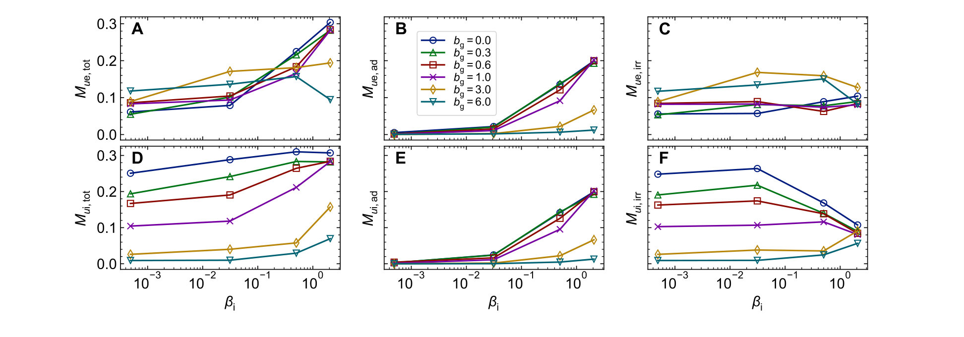 Figure 7
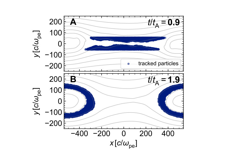 Figure 8
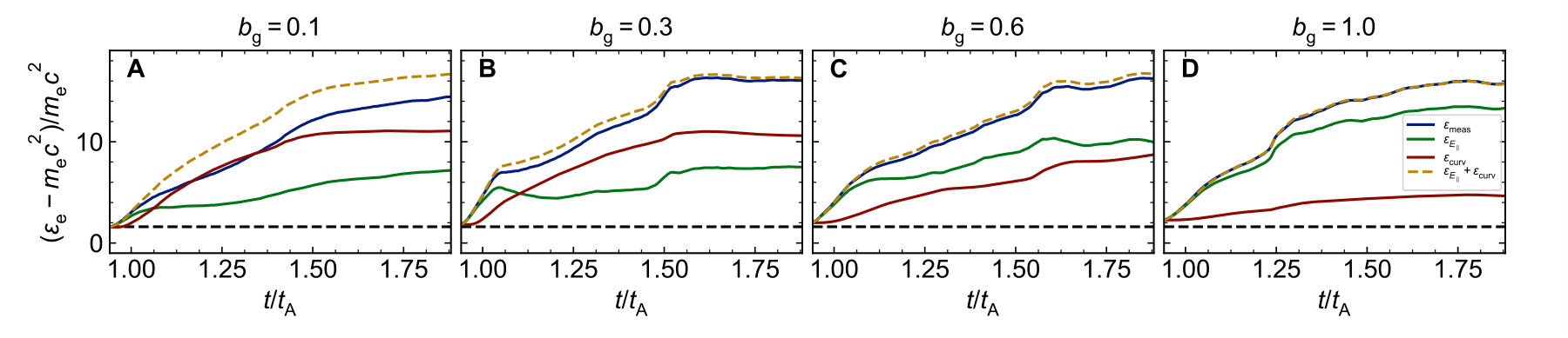 Figure 9
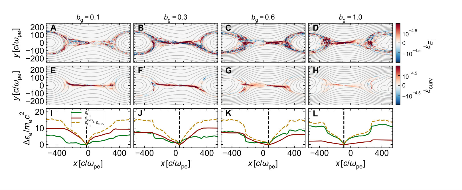 Figure 10
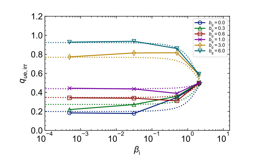 Figure 11
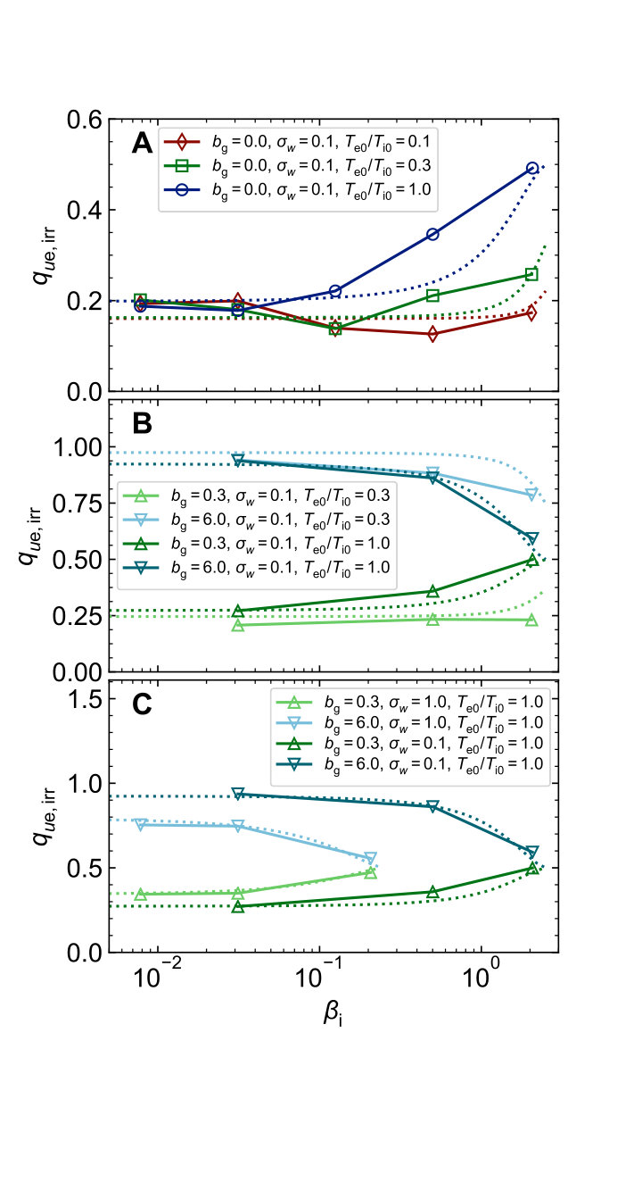 Figure 12
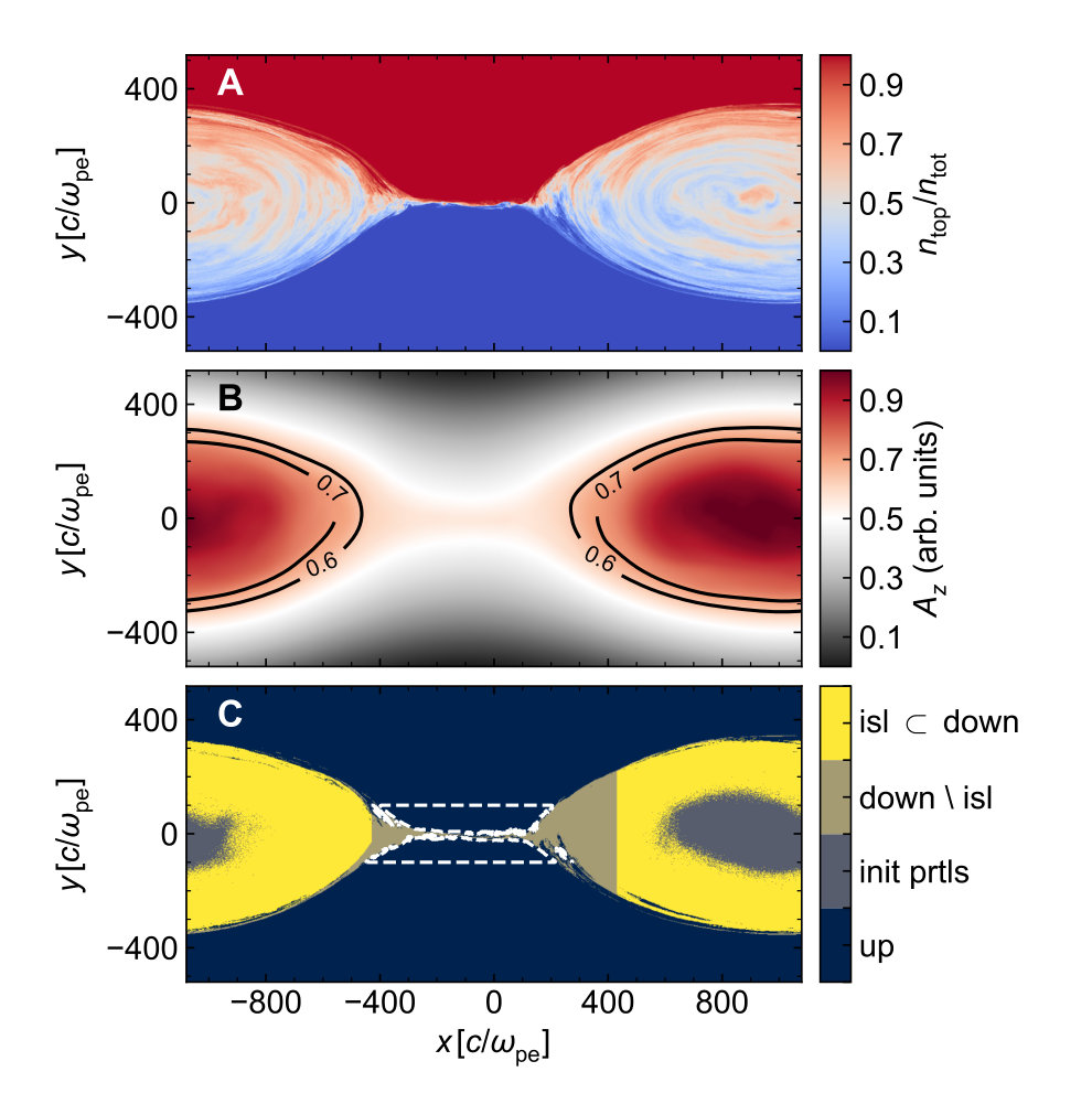 Figure 13
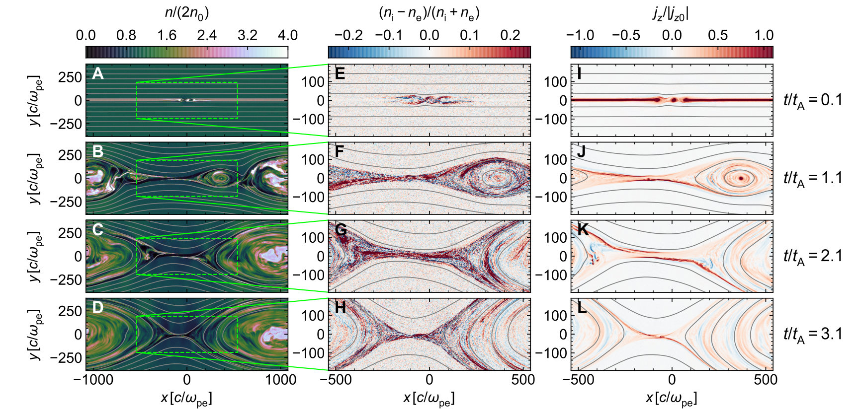 Figure 14
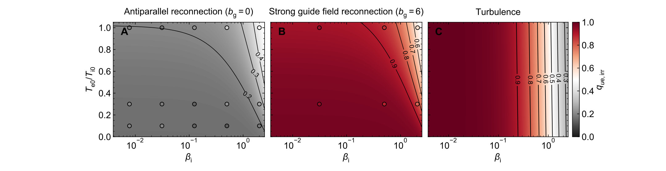 Figure 15
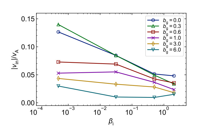 Figure 16
|
b5e-4.bg0 0 0.045 0.1 16 170 0.063 2.6 51 b3e-2.bg0 0.031 0 0.0016 2.9 0.1 16 58 0.5 7.2 149 b5e-1.bg0 0.5 0 0.031 55 0.12 16 14 2.0 6.7 617 b2.bg0 2.0 0 0.39 690 0.36 64 5.0 4.0 4.9 1728 | |||||||||||
|---|---|---|---|---|---|---|---|---|---|---|---|---|
|
b5e-4.bg3e-1 0.3 0.060 2.5 b3e-2.bg3e-1 0.3 0.48 6.9 b5e-1.bg3e-1 0.3 1.9 6.4 b2.bg3e-1 0.3 3.8 4.7 | |||||||||||
|
b5e-4.bg6e-1 0.6 0.053 2.2 b3e-2.bg6e-1 0.6 0.43 6.2 b5e-1.bg6e-1 0.6 1.7 5.8 b2.bg6e-1 0.6 3.4 4.2 | |||||||||||
|
b5e-4.bg1 1 0.045 1.8 b3e-2.bg1 1 0.35 5.1 b5e-1.bg1 1 1.4 4.7 b2.bg1 1 2.8 3.5 | |||||||||||
|
b5e-4.bg3 3 0.02 0.82 b3e-2.bg3 3 0.16 2.3 b5e-1.bg3 3 0.63 2.1 b2.bg3 3 1.3 1.6 | |||||||||||
|
b5e-4.bg6 6 0.010 0.43 b3e-2.bg6 6 0.082 1.2 b5e-1.bg6 6 0.33 1.1 b2.bg6 6 0.66 0.81 |
|
b8e-3.bg0.t1e-1 0 0.1 0.1 b3e-2.bg0.t1e-1 0.031 0 0.1 0.1 b1e-1.bg0.t1e-1 0.13 0 0.1 0.1 b5e-1.bg0.t1e-1 0.5 0 0.1 0.1 b2.bg0.t1e-1 2 0 0.1 0.1 | |||||
|---|---|---|---|---|---|---|
|
b8e-3.bg0.t3e-1 0 0.1 0.3 b3e-2.bg0.t3e-1 0.031 0 0.1 0.3 b1e-1.bg0.t3e-1 0.13 0 0.1 0.3 b5e-1.bg0.t3e-1 0.5 0 0.1 0.3 b2.bg0.t3e-1 2 0 0.1 0.3 | |||||
|
b3e-2.bg3e-1.t3e-1 0.031 0.3 0.1 0.3 b5e-1.bg3e-1.t3e-1 0.5 0.3 0.1 0.3 b2.bg3e-1.t3e-1 2 0.3 0.1 0.3 b3e-2.bg6.t3e-1 0.031 6 0.1 0.3 b5e-1.bg6.t3e-1 0.5 6 0.1 0.3 b2.bg6.t3e-1 2 6 0.1 0.3 | |||||
|
b8e-3.bg3e-1.s1 0.3 1 1 b3e-2.bg3e-1.s1 0.031 0.3 1 1 b2e-1.bg3e-1.s1 0.2 0.3 1 1 b8e-3.bg6.s1 6 1 1 b3e-2.bg6.s1 0.031 6 1 1 b2e-1.bg6.s1 0.2 6 1 1 |
Peer Reviews
No public reviews on file for this paper yet. If you reviewed it on a platform where reviews are public (OpenReview, ICLR, NeurIPS, ICML), you can paste yours below so the community can read it here.
Videos
No videos yet. Explain this paper in a talk, walkthrough, or lecture? Add one.
Electron and Proton Heating in Transrelativistic Guide Field Reconnection
Michael E. Rowan,1 Lorenzo Sironi,2 and Ramesh Narayan1
1Harvard-Smithsonian Center for Astrophysics, 60 Garden Street, Cambridge, MA 02138, USA
2Department of Astronomy, Columbia University, 550 W 120th St, New York, NY 10027, USA
Abstract
The plasma in low-luminosity accretion flows, such as the one around the black hole at the center of M87 or Sgr A* at our Galactic Center, is expected to be collisioness and two-temperature, with protons hotter than electrons. Here, particle heating is expected to be controlled by magnetic reconnection in the transrelativistic regime , where the magnetization is the ratio of magnetic energy density to plasma enthalpy density. By means of large-scale 2D particle-in-cell simulations, we explore for a fiducial how the dissipated magnetic energy gets partitioned between electrons and protons, as a function of (the ratio of proton thermal pressure to magnetic pressure) and of the strength of a guide field perpendicular to the reversing field . At low , we find that the fraction of initial magnetic energy per particle converted into electron irreversible heat is nearly independent of , whereas protons get heated much less with increasing . As a result, for large , electrons receive the overwhelming majority of irreversible particle heating ( for ). This is significantly different than the antiparallel case , in which electron irreversible heating accounts for only of the total particle heating (Rowan et al., 2017). At , when both species start already relativistically hot (for our fiducial ), electrons and protons each receive of the irreversible particle heating, regardless of the guide field strength. Our results provide important insights into the plasma physics of electron and proton heating in hot accretion flows around supermassive black holes.
Subject headings:
magnetic reconnection – magnetic fields – accretion, accretion disks – galaxies: jets – radiation mechanisms: non-thermal – acceleration of particles
††slugcomment: Accepted to ApJ: 2019 January 30
1. Introduction
When black holes accrete at much below the Eddington limit they tend to be radiatively inefficient, and the resulting accretion flows become extremely hot (see Yuan & Narayan 2014 for a review). Hot accretion flows are particularly common in the large population of low-luminosity active galactic nuclei (Ho 2008). Two members of this population, viz., Sagittarius A∗ (Sgr A∗)—the black hole at the center of our Galaxy—and the supermassive black hole in M87, are primary targets of the Event Horizon Telescope (EHT, Doeleman et al. 2008, 2009), and are of special interest at the present time. These systems, and many others like them, can be modeled within the framework of advection-dominated accretion flows (ADAFs, Narayan & Yi 1995; alternatively, radiatively inefficient accretion flows, RIAFs, Stone et al. 1999; Igumenshchev et al. 2003; Beckwith et al. 2008). However, detailed models, suitable for comparison with observations, require an understanding of electron heating in the accreting plasma, given that the observed emission is powered by electrons; yet, a detailed understanding of electron microphysics is currently lacking.
The key feature of a hot accretion flow is that the accreting gas heats up close to the virial temperature, causing the flow to puff up into a geometrically thick configuration and the plasma to become optically thin. Because of the low gas density, the plasma is largely collisionless, i.e., Coulomb collisions between charged particles are negligible. Furthermore, at radii inside a few hundred , where is the mass of the black hole and is the Schwarzschild radius, the plasma becomes two-temperature, with the protons substantially hotter than the electrons (Yuan et al., 2003). The two-temperature nature of the gas in an ADAF is a generic prediction for several reasons: first, electrons radiate much more efficiently than protons. Second, coupling between protons and electrons via Coulomb collisions is inefficient at low densities. Lastly, compressive heating favors nonrelativistic protons over relativistic electrons.
Despite these strong reasons, the plasma could still be driven to a single-temperature state if there were additional modes of energy transfer (beyond Coulomb collisions) from protons to electrons. Several mechanisms of energy transfer in collisionless accretion flows have been proposed, including weak shocks, turbulence, and magnetic reconnection (Quataert & Gruzinov, 1999; Howes, 2010; Yuan et al., 2002; Sironi & Narayan, 2015; Sironi, 2015; Werner et al., 2016; Rowan et al., 2017; Kawazura et al., 2019; Zhdankin et al., 2018). In the present work, we focus on the last of these possibilities, i.e., magnetic reconnection.
Magnetic reconnection plays an important role in the energy dynamics of numerous astrophysical systems, for example, relativistic jets, hot accretion flows (ADAFs), and coronae above stellar and accretion disk photospheres. Many of these systems tend to be magnetically dominated, in the sense that (here, is the thermal pressure of protons, with density and temperature , and is the magnetic pressure, with the magnitude of the reconnecting magnetic field). As a result, the magnetic field is the primary (or at least major) energy reservoir, and energy dissipation may proceed via reconnection. Although hot accretion flows and disk coronae are magnetically dominated (i.e., low-beta plasmas), the magnetization is typically small, with ; here, is the enthalpy density per unit volume, and and are the rest-mass densities, adiabatic indices, and internal energy densities, respectively, of electrons and protons. This regime of and , termed transrelativistic, provides a unique context for the study of magnetic reconnection, as protons are generally nonrelativistic, whereas electrons can be moderately or even ultra-relativistic (Melzani et al., 2014; Werner et al., 2016; Ball et al., 2018).
In a previous work, we explored electron and proton heating in transrelativistic reconnection, for the idealized case of antiparallel fields (Rowan et al., 2017, hereafter RSN17). The important question of electron and proton heating has been addressed by others as well, especially in the case of antiparallel reconnection (Melzani et al., 2014; Shay et al., 2014; Werner et al., 2016; Hoshino, 2018). The more general, and astrophysically relevant, case of reconnection includes a guide magnetic field component perpendicular to the plane of the reconnecting field lines. In fact, recent work suggests that turbulent heating at microscopic dissipation scales may be ultimately mediated by reconnection (Boldyrev & Loureiro, 2017; Loureiro & Boldyrev, 2017; Mallet et al., 2017; Comisso & Sironi, 2018; Shay et al., 2018). In turbulent systems like accretion flows, turbulent eddies get naturally stretched into thin current sheets, which at small scales become susceptible to the tearing mode instability, which in turn drives reconnection. At sufficiently small scales, one may then expect that energy dissipation in turbulence is mediated by reconnection. At these small scales, the guide field has the same strength as at large scales, yet the strength of the reversing fields becomes smaller at progressively smaller scales in the turbulent cascade. Our work, which focuses on guide field reconnection (up to the regime of strong guide fields), has then broader implications for energy dissipation in a turbulent cascade.
In nonrelativistic reconnection, it has been demonstrated through direct measurements, fully-kinetic and gyrokinetic simulations, and analytical theory, that the strength of the guide field heavily impacts the energy partition between electrons and protons. In the strong guide field limit, electrons receive a larger fraction of dissipated magnetic energy than protons (Dahlin et al., 2014; Numata & Loureiro, 2015; Eastwood et al., 2018). However, for the transrelativistic electron-proton plasma relevant to hot accretion flows and disk coronae, the question is under-explored, yet crucially important for obtaining predictions that can be compared to observations.
To explore the effect of a guide field in transrelativistic reconnection, we use fully-kinetic particle-in-cell (PIC) simulations, which are capable of capturing the fundamental plasma physics that controls electron and proton heating in collisionless systems. The PIC method captures from first principles the interplay between charged particles and electromagnetic fields at the basis of reconnection, thereby resolving plasma processes that are out of reach for large-scale magnetohydrodynamic simulations of accretion disks.
In this paper, we investigate the effect of a guide field on electron and proton heating via reconnection in the transrelativistic regime. We study the dependence of the heating efficiency on the initial plasma properties, by varying the guide field strength and the proton-. For our main runs, we choose as our fiducial magnetization, and the initial electron-to-proton temperature ratio is set to . In a few selected cases, we also vary the temperature ratio ( and ), as well as the magnetization (). We employ the realistic mass ratio in all our simulations.
The rest of this paper is organized as follows. In Section 2, we describe the setup and initial conditions of our simulations. Next, in Section 3, we explain our technique for measuring electron and proton heating at late times, when the energy of bulk motions driven by reconnection has thermalized. Then, in Section 4, we summarize the main results of electron and proton heating in guide field reconnection. We conclude in Section 5.
2. Simulation setup
We use the electromagnetic PIC code TRISTAN-MP (Spitkovsky, 2005), which is a parallel version of TRISTAN (Buneman, 1993), to perform numerical simulations of magnetic reconnection. Our simulations are two-dimensional (2D) in space, however all three components of particle momenta and electromagnetic fields are evolved. In this section, we describe the setup for our simulations of guide field reconnection. The simulation setup is similar to that described in Sironi & Spitkovsky (2014), RSN17, and Ball et al. (2018) for the study of antiparallel reconnection.
Simulation coordinates are as follows: the plane is the simulation plane; the antiparallel field is along , and the inflow direction is along ; a guide component of magnetic field points in the direction.
The profile of the antiparallel component of magnetic field is set as . The parameter controls the width over which the antiparallel field reverses; we usually set , where is the electron skin depth,
[TABLE]
Here, is the electron mass (including relativistic inertia), , is the initial electron internal energy density, is the number density of electrons (as well as protons) in the inflow, and is the electron charge. In all simulations, we use (we refer to RSN17 for tests of convergence with respect to the choice of ). The magnitude of the antiparallel magnetic field is controlled via the magnetization
[TABLE]
where
[TABLE]
is the specific enthalpy density of the inflowing plasma; , are the initial adiabatic indices, and , are the initial internal energy densities of electrons and protons. This definition of magnetization differs (only when plasma is relativistically hot) from the one commonly used in studies of nonrelativistic reconnection,
[TABLE]
For nonrelativistic temperatures , however for relativistically hot plasma, Eq. (2) includes the effects of relativistic inertia in the denominator, so that in general. In our simulations, we fix (except for a few cases with , which we explore in Sec. 4.4).
In addition to the antiparallel field, a guide magnetic field component is initialized perpendicular to the plane of antiparallel field lines, i.e., . The strength of the guide field is parametrized by the ratio
[TABLE]
where is the magnitude of the guide field (uniform throughout the domain) and is the magnitude of the antiparallel field. We vary from 0 to 6 (i.e., from the antiparallel case to the strong guide field regime).
Particles in the upstream region are initialized according to a Maxwell-Jüttner distribution,
[TABLE]
where , , is the initial dimensionless temperature of the respective particle species: and . The combination of proton dimensionless temperature and magnetization determines the value of proton-,
[TABLE]
Our simulations have in the range to 2. For each value, we explore a range of between and 6.
Magnetic pressure within the current sheet is smaller than that on the outside. To ensure pressure balance, a population of hot and overdense particles is initialized in the current sheet. From the pressure equilibrium condition, the temperature of overdense particles in the current sheet, , is given by where is the overdensity of particles in the current sheet, relative to that of the inflowing plasma, . We use . Electrons and protons in the current sheet are assumed to have the same temperature.
Parameters associated with each of the main runs are indicated in Tab. 1. In these simulations, we employ the physical mass ratio, , and an initial electron-to-proton temperature ratio in the upstream of . In two cases (see Sec. 4.4), we also consider and , to illustrate the dependence of our results on temperature ratio.
Reconnection is triggered at the center of the box (, ), by artificially removing the pressure of the hot particles initialized in the current sheet. This leads to the formation of an X-point. From this central X-point, the tension of reconnected field lines ejects the plasma to the left and to the right, along . We use periodic boundary conditions along , so the outflows from the two sides (i.e., the moving plasma ejected along by the field line tension) meet at the boundary, where their collision forms a large magnetic island (we shall call it “primary island” or “boundary island”). Here, particles and magnetic flux accumulate, as more plasma reconnects and is ejected along the outflows (this is discussed in detail in Sec. 3.1). Along the boundaries, we use two moving injectors (each receding from at the speed of light) to introduce fresh plasma and magnetic field; the domain is enlarged when the injectors reach the boundaries. We refer to RSN17 for further details.
In the present work, we measure electron and proton heating at late times, when the particle internal energies have reached quasi-steady values.111Thanks to our choice of periodic boundary conditions along , we are able to track the particle energies for extended times, and thus assess the time-asymptotic heating efficiency. The primary island is the site where we extract our heating measurements, which requires to run the simulations for a sufficient time such that the outflows from opposite sides of the central X-point meet at the boundary and form the island. The choice of extracting our heating efficiencies from particles residing in the primary island has advantages and disadvantages. The main disadvantage is that it does not allow to directly probe the heating that results solely from reconnection physics (which was the focus of RSN17), as it includes, e.g., heating due to shocks generated by the colliding reconnection outflows. On the other hand, our choice is the most appropriate for modeling realistic macroscopic systems, since reconnection outflows are expected to eventually come to rest, and their bulk energy to thermalize (e.g., this is expected in systems like accretion flows, for which the dynamical time and length scales are much larger as compared to that of the reconnection microphysics).
We run our simulations up to where is the Alfvénic crossing time for a box of length along the direction; is the Alfvén speed.222Note that this definition does not include the effective inertia of the guide field, which could be accounted for by defining an effective Alfvén speed as . In all the cases considered here (even the high guide field cases , for which the onset of reconnection is delayed due to the large magnetic pressure in the current sheet), we find that evolving the system for around 3–4 Alfvénic crossing times is sufficient for the measured temperatures in the primary island to attain quasi-steady values. The procedure for measuring the heating efficiency is further described in Sec. 3.
We find that the time-asymptotic heating efficiencies (especially for protons) are sensitive to the -extent of the domain, if the box is not large enough. In this case, plasma that is ejected along , away from the center, does not have enough time to reach the expected terminal velocity before stopping at the boundaries. It follows that particle heating in the primary island (which also includes the contribution from thermalization of bulk outflow energy) can be artificially inhibited if the domain is too small. We find that a box size is large enough to guard against this effect, and this is the value we use in our simulations; convergence of our heating results with respect to the domain size is discussed in App. A. In units of the proton skin depth,
[TABLE]
the adopted box size corresponds to at least , with this lower limit achieved at low . For higher values of , the proton skin depth approaches the electron skin depth, and the -extent of the domain approaches . For each value of , the box size , in units of , is listed in Tab. 1.
We use a sufficient number of computational particles per cell to ensure that numerical heating is negligible with respect to measured heating efficiencies (see Sec. 4.3; we refer also to RSN17 for convergence tests). For in the range to , we use , and for , we use a larger value, .
3. Measurement of late-time heating
In Sec. 3.1 we discuss the time evolution of the reconnection layer, and in Sec. 3.2 we discuss the measurement of late-time heating in the primary island.
3.1. Time Evolution of the Reconnection Layer
In LABEL:time_evol2, we show snapshots covering the time range – for a simulation with and moderate guide field, (run b5e-4.bg1 in Tab. 1). In the first, second, and third columns, respectively, we show the number density (in units of total upstream density, ), the degree of charge non-neutrality (i.e., the ratio of charge density to particle number density, ), and the -component of current density, normalized to the initial value in the current layer, ; the gray contours show magnetic field lines.
The time evolution is illustrated from the first to the fourth row (e.g., panels A–D). After reconnection is triggered at , an X-point forms. From the central X-point, two reconnection fronts, dragged by magnetic tension, recede from the center; for the simulation shown in LABEL:time_evol2, the speed of recession is , so the expected Alfvén limit is saturated. Since we use periodic boundary conditions, the receding fronts meet at after about one Alfvénic crossing time (second row), and merge into a volume of particles and magnetic flux that continues to grow as reconnection proceeds. As anticipated, we refer to this structure as the primary island; it is the main site where we extract our heating measurements, since this is where particles ejected from the outflow region eventually end up. Up to the runtimes of our simulations, the primary island tends to maintain an oblong shape (elongated along ), a feature that is more prominent for stronger guide fields.
Secondary islands, as opposed to the primary island, form frequently at low in the exhaust region (or equivalently, in the outflow region); the formation of secondary islands is suppressed at high (Daughton & Karimabadi, 2007; Uzdensky et al., 2010; RSN17). We find that simulations with high guide fields are characterized by a relative absence of secondary islands, as compared to simulations with the same but weaker guide fields.
The current layer in guide field reconnection is characterized by left-right and top-bottom asymmetry, especially in the exhaust region, immediately downstream of the central X-point. Electrons and protons are ejected from the X-point toward different directions: for our magnetic geometry, electrons to the upper-left and lower-right quadrants, whereas protons are sent to the upper-right and lower-left ones (see panels E–H, which zoom into the central region of panels A–D) (Zenitani & Hoshino, 2008). The -current (third column) is inhomogeneous in the immediate downstream (see panels I–L); there is some enhancement along the walls of the exhaust (at the interface with the upstream), in particular along the directions that electrons leave the X-point.
3.2. Measurement of Particle Heating in the Primary Island
To assess the heating efficiency at late times, we focus on the change in particle internal energy, as particles travel from the inflow region (i.e., the upstream) to the far downstream, and eventually enter the primary island (these different regions are defined in more detail below). Internal energy and temperature in each cell of the simulation domain are calculated as in RSN17; here we briefly review the method, but we refer the reader to RSN17 for more details.
The internal energy is computed by treating the plasma as a perfect, isotropic fluid,333Though we assume isotropy here, our measurements are not significantly affected by this assumption, as we discuss in Sec. 4.6. whose stress-energy tensor is:
[TABLE]
where e_{s}{=}\hbox to0.0pt{\hskip 0.50116pt\leavevmode\hbox{\set@color\overline{\hbox{}}}\hss}{\leavevmode\hbox{\set@colorn}}_{s}m_{s}c^{2}+u_{s},p_{s},U^{\mu}_{s}, and are the rest-frame energy density, pressure, dimensionless four-velocity, and flat-space Minkowski metric, and the subscript denotes the particle species; \hbox to0.0pt{\hskip 0.50116pt\leavevmode\hbox{\set@color\overline{\hbox{}}}\hss}{\leavevmode\hbox{\set@colorn}}_{s} is the rest-frame particle number density. From Eq. (9), the dimensionless internal energy per particle in the fluid rest frame can be written as
[TABLE]
Here,444To employ Eqs. 9 and 10, one must choose which frame to boost to; the rest-frame stress-energy tensor is computed from the lab-frame one via Lorentz transformations, , where is the local fluid velocity. This does not necessarily ensure that , so we have tested a more precise, also more expensive, calculation, i.e., solving for from , subject to the constraints (by symmetry of the stress-energy tensor, these are three equations). The solution of these equations yields a boost which ensures . However, whether we boost to the frame defined by or , our results are unchanged. is the lab-frame energy density, is the lab-frame particle number density, is the Lorentz factor computed from the local fluid velocity, is the adiabatic index, and the subscript indicates the type of particle (electron or proton). Note that the adiabatic index is a function of the specific internal energy. Given a mapping between the specific internal energy and adiabatic index, Eq. (10) can be solved iteratively for . For adiabatic index, we use a function of the form
[TABLE]
where , and . The numerical coefficients satisfy and in the nonrelativistic () and ultra-relativistic () limits, respectively; see Eq. 14 of RSN17 for additional details. The adiabatic index in Eq. (11) is used to convert between specific dimensionless internal energy and dimensionless temperature: .
In the following, we refer to “downstream” as the combination of the outflow region and the primary island. We select only part of the downstream to compute the late-time particle heating, in particular part of the primary island, which is far from the central X-point. The region is selected based on three criteria: (i) the mixing between particles originating from the top () and bottom () of the domain must exceed a chosen threshold (and be less than the complementary threshold): (RSN17), (ii) the -component of the magnetic vector potential must exceed a value, , which is related to the mixing threshold identified in (i) (Li et al., 2017; Ball et al., 2018), and (iii) cells containing particles that were part of the hot, overdense population initialized in the current sheet (see Sec. 2) are excluded, since their properties depend on arbitrary choices at initialization. The use of the above criteria for selection of the “island” region is illustrated in LABEL:rec_isl. Panel A shows the ratio of density of particles originating from the top of the domain, , to the total density . The part of the downstream that has mixed, according to (i) above, is shown in panel C by the combination of grey, yellow and tan regions.
To select the island area, which is a subset of the mixed region, we find cells at the boundary that satisfy , and of those cells, we select the ones at the upper and lower edges of the island (along ). In these cells, we compute the average value of the vector potential , to serve as a second threshold for selection of the island region (panel B). The island cells are then identified as those where there is sufficient mixing (criterion (i)), and where (criterion (ii)). We also impose a strict spatial cutoff on the island region, to ensure that it is distinct from the exhaust even at late times (see RSN17 for details). This criterion corresponds in panel C of LABEL:rec_isl to excluding the tan regions at . Finally, from the island region, we exclude any cells where the density of the hot, overdense particles used for initialization (see Sec. 2) is greater than zero (criterion (iii)), so that the measured heating does not depend on particles whose properties are set by hand as initial conditions. These initial particles generally reside in the island center (see the grey core in panel C). The region that satisfies all our criteria (which we shall call “island region” for brevity) is shown in panel C of LABEL:rec_isl as the yellow area.
The method of island selection outlined here is a robust and consistent way of selecting cells that are far downstream of the central X-point, for all guide field strengths we consider, and it is relatively insensitive to the choice of threshold value . For example, differs by no more than for in the range –; the overall measured values of particle heating in the island show comparable sensitivity to the choice of , at a level of around for in the range –. For island selection, we find that is suitable.
To assess particle heating, we measure the change in particle internal energies, as they travel from the inflow to the island region (described above). The upstream region is defined such that or (so, a complementary definition to the mixing criterion (i) above). We employ a threshold value ; the fact that provides a thin (few ) buffer region between the downstream (tan and yellow areas combined in panel C of LABEL:rec_isl) and the upstream (navy region in panel C of LABEL:rec_isl). We further select only those upstream cells lying within of (as delimited by the dashed white contours in panel C of LABEL:rec_isl).
With the inflow and island regions suitably identified, overall heating fractions can be computed as the difference between the dimensionless internal energies in the island and inflow regions, normalized to the inflowing magnetic energy per particle (Shay et al., 2014; RSN17):
[TABLE]
These dimensionless ratios indicate the fraction of magnetic energy per particle in the inflow that is converted to particle heating, by the time the particle reaches the island, far downstream of the central X-point. As in RSN17, the heating fractions in Eqs. 12 and 13 can be decomposed into adiabatic-compressive and irreversible components,
[TABLE]
The adiabatic heating fractions represent the heating that results solely from an increase in internal energy due to adiabatic compression of the plasma as it travels from the inflow to the island; for electrons, the adiabatic heating fraction is approximately555This is an approximation because Eq. (16) assumes a constant adiabatic index ; in reality, when calculating , we properly account for the possibility of a changing adiabatic index, as is appropriate for electrons that start nonrelativistic in the upstream, but are heated to ultra-relativistic temperatures by the time they reach the island. (RSN17)
[TABLE]
where is the typical electron density in the island. The irreversible heating fractions are associated with a genuine increase in the entropy of the particles, and are of primary interest to us. The measured heating fractions we present in Sec. 4 are typically time-averaged over one Alfvénic crossing time ().
A representative temporal evolution of electron and proton irreversible heating fractions, and , is shown in LABEL:mu_bth_timeseries. The time evolution of the heating fractions is shown from to ; at late times, the heating fractions achieve a steady state (i.e., both the electron and proton irreversible heating fractions are relatively flat after ). Time-averaged heating fractions are computed during this steady state; the points used for time-averaging are indicated by the shaded region in LABEL:mu_bth_timeseries.
4. Results
In this section, we discuss our measurements of electron and proton heating in the primary island, and their dependence on guide field strength and upstream proton-. In Sec. 4.1, we focus on one low and one high case, and explore the effect of guide field strengths in the range 0.3–6. Next, in Sec. 4.2, we show the dependence of the reconnection rate on and the guide field. In Sec. 4.3, we present comprehensive results of electron and proton heating, extracted from a suite of simulations that span the whole parameter space 0–6 and –. Here, we focus on the case of equal initial electron and proton temperatures in the upstream, . For these simulations, the magnetization is . In Sec. 4.4, we present several results of irreversible electron heating from simulations with temperature ratios in the range –, as well as several cases with . Next, in Sec. 4.5, we a provide a fitting function for the electron irreversible heating efficiency, based on the simulation results presented in Secs. 4.3 and 4.4. Then, in Sec. 4.6, we discuss the degree of anisotropy in the particle distribution (as a function of and ), and its effect on the accuracy of our results. Lastly, in Sec. 4.7, we discuss an application of the guiding-center formalism to dissect the mechanisms responsible for electron heating at low .
4.1. Electron and Proton Heating: Weak vs. Strong Guide Field
Electron and proton heating via reconnection shows substantial differences in the limits of strong and weak guide field. LABEL:gf_compare2 shows 2D snapshots at of electron (panels A–C) and proton (panels D–F) temperature,666Here, we phrase our results in terms of temperature, rather than internal energy; however, similar conclusions hold regardless of which quantity is considered (in this section as well as in the rest of the paper). and corresponding 1D profiles (panels G–I), for three simulations with a relatively low and guide field strengths and , increasing from left to right. The simulations here correspond to runs b3e-2.bg3e-1, b3e-2.bg1, and b3e-2.bg6 in Tab. 1.
The first and second rows show the spatial dependence of electron (panels A–C) and proton (panels D–F) heating. At low (run b3e-2.bg3e-1), the electron and proton temperatures are relatively uniform in the exhaust and island regions. For intermediate guide field strengths (run b3e-2.bg1), the electron and proton heating is less uniform in the island, and shows marked a asymmetry in the exhaust region (see panels B and E, in between the cyan lines). For the strong guide field case (run b3e-2.bg6), electrons reach a maximum temperature of roughly along the upper-left and lower-right edges of the outflow; on the other hand, proton heating along the exhaust is essentially isolated to the upper-right and lower-left edges. Throughout the entire downstream (for run b3e-2.bg6), the proton temperature rarely exceeds .
The 2D plots in panels A–F also illustrate that the primary island becomes more oblong with increasing guide field. For , the aspect ratio of the island (length along the layer to width orthogonal to it) is about , whereas at , it is twice as large, . In the cases with strong guide field the primary islands do not circularize up to the run times of our simulations.
The bottom row of LABEL:gf_compare2 shows the 1D profiles of electron (blue) and proton (red) temperatures, both in units of , averaged along for cells within the downstream region (including the yellow and tan regions in panel C of LABEL:rec_isl, and excluding the grey area in the island core that contains particles left over from initialization). The edges of the primary island are shown by vertical cyan lines. Horizontal black dashed lines indicate the initial temperature of particles in the far upstream. In the weak guide field case (panel G), protons are heated substantially more than electrons, similar to the case of antiparallel reconnection (see Melzani et al. (2014), Werner et al. (2016), RSN17). As the strength of the guide field increases (panels H and I), proton heating in both the exhaust region and the primary island is strongly suppressed. The electron temperature, on the other hand, is largely unaffected; for and , the electron temperature in the island is always around .
LABEL:gf_compare3 is similar to LABEL:gf_compare2, but corresponds to a set of simulations with (runs b2.bg3e-1, b2.bg1, and b2.bg6 in Tab. 1). As we discuss below, this value of is close to (see Eq. (18)), impliying that electrons and protons both start with relativistic temperatures. In stark contrast to the low case, at the electron and proton temperatures in the island region are roughly equal, regardless of the guide field strength (–). Still, the 2D temperature structure within the island differs between low and high guide field cases. At high and low or intermediate guide field (runs b2.bg3e-1 and run b2.bg1), the electron and proton temperatures in the island are typically uniform (similar to the low , low case in panels A and D of LABEL:gf_compare2). However, at high and high guide field (run b2.bg6), the electron and proton temperatures are less uniform (relative to runs b2.bg3e-1 and b2.bg1; see panels C and F of LABEL:gf_compare2), with electron and proton temperatures greatest near the interfaces between the primary island and the outflows (i.e., ).
4.2. Reconnection Rate
LABEL:vinvout_bth shows the and dependence of the reconnection rate, . The inflow speed is computed as a spatial average over a specific region of the upstream,777Specifically, in the region where and . and temporal average from to (when reconnection is roughly in steady state). Each point corresponds to the measurement from a different simulation, and those with the same guide field strength are connected by a solid line. For these simulations, , , and .
In most cases, reconnection proceeds at or below the value often reported in the literature, i.e. (Cassak et al., 2017); however, for low and weak guide field (), the reconnection rate exceeds this fiducial value, with in the range 0.1–0.15. For , the reconnection rate shows a relatively weak scaling with , decreasing from – to , only a factor of 2–3, as increases from to (Numata & Loureiro, 2015, RSN17, Ball et al., 2018). For guide fields , the dependence of the reconnection rate is even weaker, and typically varies from 0.01 to 0.07. We find that the presence of a guide field tends to suppress the reconnection rate, which is a dependence similar to that found by Melzani et al. (2014) for electron-ion relativistic reconnection, Ricci et al. (2003), Huba (2005), TenBarge et al. (2013), and Liu et al. (2014) for electron-ion nonrelativistic reconnection, and Hesse & Zenitani (2007) and Werner & Uzdensky (2017) for electron-positron plasma. The decrease in the reconnection rate with is more pronounced at lower values of .
4.3. Electron and Proton Heating: and Dependence
LABEL:dindout_bth shows the and dependence of electron (panel A) and proton (panel B) dimensionless temperature. Each solid line shows the volume-averaged temperature in the island for a set of simulations with the same value of , and the black diamonds, connected with a dashed line, show the upstream temperature for each value of (for simulations with fixed , the upstream temperature is the same, independent of ). As discussed in Sec. 2, the numerical resolution is sufficient to keep numerical heating under control; temperatures measured in the inflow region are about the same as the ones at initialization, throughout the duration of our simulations.888Due to numerical heating, the measured upstream temperature for the runs differs from the expected initialized electron temperature, (see Tab. 1). However, the difference is much smaller (less than ) in runs with higher . Although the upstream numerical heating for is large compared to the temperature at initialization, the resulting upstream temperature is still much smaller than the downstream temperature, so it has no effect on the heating fractions presented below. The basic reason is that for low , the available magnetic energy (a fraction of which will be transferred to the particles) is much larger than the initial particle thermal energy. The simulations presented here are the same as those in Sec. 4.2, so they employ , , and .
The upstream electron dimensionless temperatures range from nonrelativistic, , up to ultra-relativistic, ; the temperatures in the downstream region range from moderately to ultra-relativistic, –.999This is a consequence of our choice of ; for , the bulk of electrons will not attain ultra-relativistic energies. For all values of , the electron temperature in the island appears to be nearly independent of the guide field strength (LABEL:dindout_bth, panel A). The guide field simulations show the same scaling with as the antiparallel case (blue circles), with the electron temperature increasing from about at up to at . Additionally, the electron temperature shows only a relatively weak dependence on , for . From up to , the electron temperature in the island changes by no more than a factor of 10 (the dependence is even weaker for ). At high , the electron temperature in the island appears to be nearly the same as that in the upstream. However, the increase in temperature from upstream to downstream corresponds to a substantial fraction (typically ) of the inflowing magnetic energy per electron (see LABEL:mu_bth below, panel A). These two statements are not in contradiction, since for high the available magnetic energy is only a small fraction of the initial thermal energy.
In LABEL:dindout_bth, panel B, we show the proton dimensionless temperature in the island, for the same simulations shown in panel A. At low , protons show a clear decrease in island temperature with increasing guide field strength; for antiparallel reconnection () and , the proton dimensionless temperature in the island is but decreases to for strong guide field, . As increases, the proton heating in the island shows a weaker dependence on guide field strength. Similar to electron heating in the island at high , is nearly independent of at high . The proton dimensionless temperatures, in both the upstream and the island region, are generally nonrelativistic, . In summary, when comparing panels A and B, a striking difference is that the electron dimensionless temperature in the island is independent of the guide field strength, whereas the proton dimensionless temperature appreciably decreases with increasing .
In LABEL:mu_bth we present the scaling of electron and proton heating with guide field strength and proton-. The first and second rows show the electron and proton heating fractions, respectively (see Eqs. 12–15); the total heating (first column) is decomposed into adiabatic-compressive and irreversible components, shown in the second and third columns, respectively. In each panel, the corresponding heating fraction is plotted as a function of for guide field strengths in the range [math]–.
The first row in LABEL:mu_bth shows the scaling of the electron total, adiabatic, and irreversible heating fractions (, and ) with respect to and . At low , the electron total heating fraction within the island does not show a strong scaling with the strength of the guide field (consistent with LABEL:dindout_bth). For , . At high , the total heating is suppressed by strong guide fields, . Some insight into this trend is provided by decomposing the total heating fraction into adiabatic and irreversible parts, (panel B) and (panel C). For low , compressive heating is negligible; however, at higher values of , compressive heating is more significant, but tends to decrease with stronger guide fields, which is in qualitative agreement with Li et al. (2018). This result is physically intuitive, as the plasma becomes less compressible when the magnetic pressure of the guide field is larger (and in fact, we notice that the primary island is less dense for stronger guide fields).
To summarize, we find that the electron compressive heating fraction in panel (B) steadily increases with and strongly decreases with . Both trends for can be easily understood from Eq. (16), given that stronger guide fields give smaller density compressions. In contrast, the electron irreversible heating fraction (panel C) is largely independent of both and , and it is around . The combination of irreversible and compressive heating explains why the total heating at low is independent of both and , whereas at high it is lower for larger (due to the corresponding trend in compressive heating).
The second row in LABEL:mu_bth shows the proton heating fractions , and (panels D, E, and F). The proton total heating in the island differs sharply from the electron total heating (panel A). The proton total heating shows a strong dependence on the strength of the guide field; for antiparallel reconnection, regardless of , but the total heating is significantly suppressed as increases. For and , is negligible. The proton compressive heating (panel E) shows a trend similar to that of the electron compressive heating (panel B); for both electrons and protons, the compressive heating is controlled by density in the upstream, density in the island region, and upstream temperature (here, we focus on the case ); since these quantities are similar for electrons and protons, the compressive heating for both species shows the same trend. The proton irreversible heating (panel F) is similar to the proton total heating (panel A) for , because compressive heating is negligible in this regime. For , the proton irreversible heating is less sensitive to the guide field strength, and by , regardless of , similarly to the electron irreversible heating.
The electron and proton irreversible heating fractions and can be used to compute the ratio of electron irreversible heating to total irreversible particle heating liberated during reconnection (RSN17),
[TABLE]
In LABEL:que_irr_bth, we present the and dependence of , the electron irreversible heating efficiency. For all , increases with the guide field strength. For antiparallel reconnection, electrons ultimately receive of the irreversible heat transferred to particles. As the guide field increases, so does the fraction of irreversible heating transferred to electrons; for , and by , electrons receive the vast majority of magnetic energy that is converted to irreversible particle heating, with . At , , independently of ; is the maximum possible value of , given and , and is defined as
[TABLE]
This equation is derived by expressing as a function of , and , then taking the limit . For the simulations presented here, with , , and , we find . Note that for , electrons and protons start relativistically hot in the upstream, and the scale separation is of order unity (RSN17); in this case, electrons and protons behave nearly the same, which explains why for we obtain energy equipartition, i.e., we find that , independently of .
\onecolumngrid
\twocolumngrid
4.4. Electron Irreversible Heating Efficiency: and Dependence
For simplicity, we focused in Sec. 4.3 on electron heating for cases with representative magnetization and temperature ratio . A full exploration of the dependence of electron and proton heating on , , , and is beyond the scope of this work. Nevertheless, for a limited range of and , we present in LABEL:que_irr_others the electron irreversible heating efficiencies when we vary the electron-to-proton temperature ratio in the range 0.1–1 (panels A and B), as well as for several simulations with (panel C). The physical parameters of these runs are given in Tab. 2.
The effect of varying the initial electron-to-proton temperature ratio for antiparallel reconnection () is demonstrated in panel A of LABEL:que_irr_others. At low , the electron irreversible heating efficiency shows nearly no dependence on or temperature ratio. At high , the dependence on temperature ratio can be understood via the dependence of on . According to Eq. (18), decreasing the temperature ratio for fixed leads to an increase in , and so (as discussed in Sec. 4.2) in the value of where equipartition between electrons and protons is realized.
The effect of varying the temperature ratio for and is shown in panel B. As for antiparallel reconnection, there is no significant dependence on at low , for each of the two values. While for , for we expect , so equipartition between electrons and protons, which should hold regardless of at , is expected at higher than probed in panel (B).
The effect of varying the magnetization and guide field strength is shown in panel C of LABEL:que_irr_others. At low , the electron irreversible heating efficiency has a weaker dependence on guide field for than for . For (see Eq. (18)), irreversible heating of electrons and protons is in equipartition, and this conclusion holds regardless of or .
4.5. Fitting function
For use as a sub-grid model of electron heating in magnetohydrodynamic simulations (as in Ressler et al. (2017); Chael et al. (2018); Ryan et al. (2018)), we provide the following fitting formula, motivated by the simulation results presented in Secs. 4.3 and 4.4:
[TABLE]
where is in Eq. (18) in terms of and .
The fitting function in Eq. (19) has the following limits: for low , asymptotes to a (- and -dependent) value that does not depend on . The asymptotic low- limit tends to the equipartition value for (i.e., in the limit of ultra-relativistic reconnection), regardless of . Still at , electrons receive most of the irreversible heat if . For , and , we get , i.e., all of the irreversible heat goes to electrons. At , the fitting function returns , independent of , , and . For in the range [math]–, the fitting function in Eq. (19) is plotted in Figs. 9 and 10 as dotted lines, showing that it matches well the trends obtained from the simulations.
Predictions of the reconnection-mediated heating model presented here differ from those of heating via a Landau-damped turbulent cascade (Howes, 2010; Kawazura et al., 2019; Zhdankin et al., 2018). In LABEL:turb_compare we show a comparison between reconnection-based heating (Eq. (19)) for the antiparallel (, panel A) and strong guide field (, panel B) cases, and the turbulence-based heating prescription of Kawazura et al. (2019) (panel C), over the range of plasma conditions we have investigated. First, one notices that turbulence-based heating is much more similar to heating via reconnection in the strong guide field limit, rather than in the antiparallel case. In fact, for the latter (in contrast to the first two), protons are heated much more than electrons at low . However, some differences persist even between turbulent heating and heating via strong guide field reconnection. In fact, the turbulence-based heating model is nearly insensitive to the initial temperature ratio , whereas for guide field reconnection, an increase in decreases (see Eq. (18)), which in turn decreases the value of at which electrons and protons achieve equipartition, i.e., . More generally, relativistic effects leave a unique fingerprint in our results at ,101010We remark that may be much larger or much smaller than unity, depending primarily on . where both species start as relativistically hot, and in the limit . In either case, protons and electrons receive equal amount of the dissipated energy, i.e., , regardless of the guide field strength.
4.6. Temperature Anisotropy
Guide field reconnection can result in highly anisotropic electron distribution functions at late times (Dahlin et al., 2014; Numata & Loureiro, 2015). Yet, to determine the dimensionless internal energy per particle in the fluid rest frame, we have assumed an isotropic stress-energy tensor at every location in the upstream and in the downstream. Eq. (10) relies on this assumption. In addition, we have implicitly assumed isotropy in our prediction for the amount of adiabatic heating.
To assess whether isotropy is a reasonable assumption, we show in LABEL:aniso_bth the electron temperature anisotropy in the island ( and refer to orientations relative to the local magnetic field); the simulations here are similar to the production runs listed in Tab. 1, but cover more densely in the range up to .
For weak guide fields (), the electron temperature is isotropic, (see RSN17). For and , we find substantial anisotropy, with temperature ratios in the range –. In these cases, isotropy is certainly not a valid assumption. As discussed above, this will affect our inferred internal energy (since, in principle, Eq. (10) cannot be employed) and the predicted degree of adiabatic heating. As regard to the internal energy, in a few cases we have calculated all the components of the stress energy tensor in the simulation frame. By transforming into the comoving frame, we do not need to rely on any assumption of isotropy. In general, we have found the inferred internal energies differ from Eq. (10) only at the level.
As regard to adiabatic heating, we have discussed in Sec. 4.3 that compressive heating is suppressed by strong guide fields, as well as at low values of . Therefore, in the majority of cases that show substantial temperature anisotropy, adiabatic heating constitutes a negligible fraction of the total heating, so the degree of anisotropy has only a negligible effect on the inferred irreversible heating. A notable exception here is the run with and , for which compressive heating accounts for about 33% of the total heating, and the measured anisotropy in the island is non-negligible, ; of all our simulations, this one has the greatest systematic uncertainty on the compressive heating, and consequently on the inferred irreversible heating.
4.7. Mechanisms of Electron Heating in Guide Field Reconnection
The orbit of a charged particle in electromagnetic fields may be approximated as the superposition of two motions: fast circular motion about a point, the guiding center, and a slow drift of the guiding center itself. This approximation is valid when the particle’s gyroperiod is short compared to the timescale of variation of the fields, and also when the particle’s Larmor radius is small compared to the field gradient length scale. When valid, the guiding center approximation can provide valuable insight into the mechanisms responsible for particle energization (see e.g., Dahlin et al. (2014); Sironi & Narayan (2015); Wang et al. (2016)). In this section, we use the guiding center approximation to investigate the mechanisms of electron heating for , as a function of the guide field strength. Details of the guiding center decomposition are discussed in App. B.
We track electrons starting initially in the upstream region (see LABEL:prtl_bth_init_final, panel A), and compute the contributions and , which correspond to energy changes due to the parallel electric field and curvature drift, respectively. For clarity we focus in our discussion only on the -parallel and curvature drift terms, which tend to dominate for the cases we investigate here (we have directly verified this, and it agrees with findings of Dahlin et al. (2014) for nonrelativistic reconnection). While the simulation timestep is , the time interval we use here for outputs of the field and electron properties for the guiding center analysis is around . To ensure that this time resolution is sufficient for a guiding center reconstruction, we compare the actual evolution of the electron energy (computed on the fly by the simulation) to the value calculated from the downsampled field and particle information. For the time range over which we track particles ( for these simulations), the energy gain computed from downsampled field and particle information shows excellent agreement with the actual value evolved at the time resolution of the simulation.
To study electron heating via the guiding center theory, we use four simulations for which and . Here, we use a smaller box size, (the domain size dependence of our results is discussed in App. A). Apart from the domain size, the parameters are the same as in the main guide field simulations (i.e., , , , cells, ). The heating fractions extracted from these simulations are roughly the same as in the production runsof Tab. 1.
Electrons are tracked from to (equivalently, to ). The tracked particles are selected at the initial time to lie in the upstream region, within roughly of (see LABEL:prtl_bth_init_final, panel A; grey contours show magnetic field lines). The selected electrons are tracked for , at which point they typically reside in the island region (panel B).
LABEL:prtl_bth shows the time evolution of electron energy gains, for guide fields , and in panels A, B, C, and D, respectively (the strength of the guide field increases from left to right). The energy gain is presented in dimensionless form with rest mass subtracted, i.e., .111111This is not an equality because includes bulk kinetic energy, in addition to internal energy. However, in the primary island the latter greatly dominates over the former. In each panel, the blue line corresponds to the electron energy gain measured directly in the simulations. The -parallel and curvature terms are shown in green and red, respectively, and the yellow dashed curve is their sum. The good agreement between dashed yellow and blue lines is an indication that our output time resolution is adequate for the guiding center reconstruction. The black dashed line shows the specific internal energy in the far upstream (), which matches well the starting point of the curves.
For weak guide fields, , the energy gains due to -parallel and curvature terms are comparable, consistent with the findings of Dahlin et al. (2014). For strong guide fields, energization due to the parallel electric field dominates; in this case, the magnetic field in the current sheet is approximately straight (since it is dominated by the out-of-plane field), so heating due to the curvature term is negligible. Though the mechanisms responsible for energization of electrons differ for weak and strong guide fields, the overall energy gain is about the same in all cases, (see also LABEL:dindout_bth, panel A). The temporal evolution of electron heating (both the total heating, as well as -parallel and curvature contributions) saturates at late times, when most of the particles reside in the primary island.
LABEL:prtl_bth_spatial shows the 2D spatial distribution of power associated with the -parallel (panels A–D) and curvature (panels E–H) energization terms. For every tracked electron at each time, we deposit the corresponding -parallel and curvature powers at the location where the particle instantaneously resides (power is deposited into spatial bins of length and width equal to ; note that the colorbar range in LABEL:prtl_bth_spatial depends on this binning, so the units are arbitrary), and then we average over the number of tracked electrons. Grey lines show the magnetic field lines at , for reference. For weak guide fields (), energization due to the parallel electric field is patchy (Dahlin et al. (2014)), with heating spread over the exhaust region as well as the island. On average, there is a net energy gain, however, parallel electric fields can also locally cool the electrons (blue patches in panel A). Heating due to the curvature drift is localized predominantly along the walls of the exhaust, in particular on the upper left and lower right (as in panel B, for ), where outflowing electrons tend to get focused (see also LABEL:time_evol2, panel F).
As the strength of the guide field increases, the relative importance of the curvature drift energization decreases (panels G–H), and the -parallel heating becomes dominant (panels C–D). A substantial amount of heating due to the parallel electric field is localized in the exhaust region, however energization continues into the island.
While the guiding center formalism makes no distinction between adiabatic and irreversible heating, we can infer based on our results for low guide field reconnection (see LABEL:mu_bth, first row) that the -parallel and curvature drift terms in this case (having ) contribute predominantly to the irreversible heating of electrons. Since compressive heating is negligible at (see LABEL:mu_bth, panel B; also, Eq. (16)), irreversible heating in the low regime represents the main contribution to total electron heating. It follows that, in this low regime, the guiding center decomposition assesses contributions to irreversible heating.
To clarify the spatial dependence of -parallel and curvature drift heating, we show in the last row of LABEL:prtl_bth_spatial (panels I–L) the 1D cumulative sum along (as in Dahlin et al. (2014)), starting from the vertical dashed line, of the -parallel (solid green) and curvature (solid red) energization rates displayed in the first and second rows; their sum is shown by the dashed yellow line. This shows that heating continues throughout the exhaust region, and at the interface between the outflow and the primary island. Little additional heating happens inside the primary island.
5. Summary and discussion
By means of fully-kinetic large-scale 2D PIC simulations, we have investigated guide field reconnection in the transrelativistic regime most relevant to black hole coronae and hot accretion flows. In particular, we have focused on the fundamental question of electron and proton heating via reconnection, differentiating between adiabatic-compressive and irreversible components. All our simulations employ the realistic mass ratio, .
We find that the energy partition between electrons and protons can vary substantially depending on the strength of the guide field. For a strong guide field and low proton beta , around of the free magnetic energy per particle is converted to irreversible electron heating (regardless of ), whereas the efficiency of irreversible proton heating is much smaller, of order (these values refer to our fiducial magnetization and temperature ratio ). It follows that the energy partition at high guide fields differs drastically from the antiparallel limit (), in which electrons receive only of the free magnetic energy per particle, and proton irreversible heating is around four times as much, (RSN17).
While the energy partition between electrons and protons changes drastically with the guide field strength at low , at (, for and ), the irreversible heating of electrons and protons is in approximate equipartition, regardless of the guide field strength. That is, as (when both species start relativistically hot), electrons and protons each receive roughly the same amount of energy, of the free magnetic energy per particle in the upstream.
In addition to a comprehensive investigation of the guide field dependence of electron and proton energy partition for our fiducial cases with and , we study several cases with larger magnetization, , and smaller temperature ratios, . Motivated by our extensive exploration of the parameter space (Tab. 1 and (Tab. 2), we provide a fitting function (Eq. (19)), which captures the approximate dependence of electron irreversible heating efficiency on , and . This fitting function can be used for sub-grid models of low-luminosity accretion flows such as Sgr A∗ at the Galactic Center.
As we have said, for strong guide fields and low , electrons receive most of the irreversible heat that is transferred to the particles. This is similar to recent findings of electron and proton heating in magnetized turbulence (see Fig. 11, which compares with Kawazura et al. 2019), suggesting a fundamental connection between reconnection and turbulence, as indeed supported by recent theoretical works (Boldyrev & Loureiro, 2017; Loureiro & Boldyrev, 2017; Mallet et al., 2017; Comisso & Sironi, 2018; Shay et al., 2018). Still, some key differences between our reconnection-based heating prescription and turbulence-based heating prescriptions (Howes, 2010; Kawazura et al., 2019) persist: for , when both electrons and protons start relativistic, reconnection leads to equipartition between the two species independently of the guide field strength, whereas for the prescription of, e.g., Kawazura et al. (2019), protons receive the majority of the irreversible heating at high . Also, for reconnection-based heating, the transition to equipartition happens not at , but generally at , which can differ from unity if or .
We have also used a guiding center analysis to study the mechanisms responsible for electron heating as a function of the guide field strength, for a representative low- case with . The -parallel and curvature drift terms dominate the energy change of electrons, and their relative importance shifts depending on the strength of the guide field; for weak to moderate guide fields, , the energy gains due to -parallel and curvature drift are comparable, but for a strong guide field, , electron energization is dominated by -parallel heating. Though the mechanisms of electron heating differ depending on the strength of the guide field, the net increase in electron energy remains about the same.
We conclude by remarking on some simplifying assumptions of the present work, as well as discussing future lines of inquiry. First, in our investigation of guide field reconnection, we have focused primarily on one value of the magnetization, , and equal temperature ratios in the upstream, ,121212The fitting function Eq. (19), however, also incorporates results from additional simulations with and , for both low and high guide field regimes. to simplify the parameter space investigation. The dependence of energy partition via reconnection on guide field strength for other values of the magnetization remains under-explored, especially for the low regime, where we find that the proton irreversible heating efficiency depends strongly on the guide field strength. Similarly, the effect of the upstream temperature ratio in guide field reconnection is under-explored.
A second simplification is that we have used 2D simulations, which may differ from 3D as regard to particle heating. In 3D reconnection, in place of magnetic islands, twisted tubes of magnetic flux will develop; to understand the differences as regard to heating, a comparison between 2D and 3D transrelativistic reconnection will be important, especially in the low- regime, where secondary magnetic islands are copiously generated.
Finally, in our guiding center analysis, we have focused on electron heating in the low regime, where the assumption that the magnetic field varies negligibly over the electron radius of gyration is easily satisfied. At high , this assumption is less robust, and the guiding center theory may be not applicable. Additional theoretical work will be necessary to provide insight into the physics of electron and proton heating in these regimes.
Acknowledgements
This work is supported in part by NASA via the TCAN award grant NNX14AB47G and by the Black Hole Initiative at Harvard University, which is supported by a grant from the Templeton Foundation. LS acknowledges support from DoE DE-SC0016542, NASA Fermi NNX-16AR75G, NASA ATP NNX-17AG21G, NSF ACI1657507, and NSF AST-1716567. The simulations were performed on Habanero at Columbia, on the BHI cluster at the Black Hole Initiative, and on NASA High-End Computing (HEC) resources. This research also used resources of the National Energy Research Scientific Computing Center, a DOE Office of Science User Facility supported by the Office of Science of the U.S. Department of Energy under Contract No. DE-AC02-05CH11231.
Appendix A Appendix A: Convergence of irreversible heating fractions with respect to domain size
The main focus of this paper is the irreversible heating of electrons and protons. In principle, the measured values may depend on the domain size if, for example, the computational box is so small that the reconnection outflows do not have the chance to reach the asymptotic Alfvén limit. In this case, the bulk energy of the outflows would be artificially suppressed, which could in turn suppress the particle irreversible heating. In this appendix, we present a set of lower resolution ( instead of ) simulations with varying domain sizes, (our fiducial choice), and , to explore the box size dependence of the electron and proton irreversible heating fractions, and . For these simulations, , , , , and . In LABEL:boxsize_conv, we show the time dependence of electron (panel A) and proton (panel B) irreversible heating fractions for the three simulations with varying .
For box sizes , the electron irreversible heating converges to . With respect to electron irreversible heating, even the smaller box with differs by only compared to the larger boxes. This justifies the fiducial domain size that we use to study electron heating in guide field reconnection, and also the choice of in Sec. 4.7, where we use the guiding center theory to study electron energization. The proton irreversible heating depends more strongly on the box size, but still shows reasonable agreement between the fiducial box size () and larger boxes (). In contrast, smaller boxes underestimate the proton heating fraction (green line).
Appendix B Appendix B: Guiding Center Formalism
In the guiding center formalism (Northrop, 1961, 1963a, 1963b), the energy change of an electron, time-averaged over the gyration period, and to first order in the expansion parameter , is
[TABLE]
where , is the electron charge, is the adiabatic moment of the electron, is the direction of the local -field, and is the drift velocity; electric and magnetic fields are to be evaluated at the location of the guiding center. The underbrackets indicate terms that are associated with parallel and perpendicular energy changes. Several of the terms have direct physical significance, and provide insight into the mechanisms responsible for particle energization, as we discuss below.
The first of the terms labeled ‘parallel’ in Eq. (B1) corresponds to acceleration by the electric field, parallel to the local -field. The second term contains the well-known ‘curvature drift’,
[TABLE]
which describes the Fermi-like acceleration of particles due to the magnetic tension of curved field lines (Drake et al., 2006, 2010). On the second line of Eq. (B1), the first term expresses energy change due to the ‘-drift’,
[TABLE]
The second term in the second line of Eq. (B1) corresponds to the induction effect of a time-varying field due to acting about the circle of gyration (Northrop, 1963b). Finally, the third term is related to energy change due to ‘polarization drift’, which is driven by time-variation in the electric field:
[TABLE]
In practice, many terms in the expansion of Eq. (B1) can be ignored, as their contribution to the electron energy gain is negligible. In Sec. 4.7, we employ the guiding center analysis, as detailed in Dahlin et al. (2014), to assess the mechanisms responsible for energy gain in guide field reconnection. Formally, the electromagnetic fields are to be evaluated at the location of the guiding center, however if the electron Larmor radius is sufficiently small, relative to the gradient length scale of the magnetic field, then the measured value at the guiding center is similar to that at the particle location. For the simulations described in Sec. 4.7, we find that this is a reasonable assumption.
The reference list from the paper itself. Each links out to its DOI / PubMed record.
- 1Ball et al. (2018) Ball, D., Sironi, S., & Özel, F. 2018, Ap J, 826, 77
- 2Beckwith et al. (2008) Beckwith, K., Hawley, J. F., & Krolik, J. H. 2008, Ap J, 678, 1180
- 3Boldyrev & Loureiro (2017) Boldyrev, S., & Loureiro, N. F. 2017, Ap J, 844, 125
- 4Buneman (1993) Buneman, O. 1993, in Computer Space Plasma Physics: Simulation Techniques and Software, ed. H. Matsumoto, Y. Omura, & E. Sindoni (Terra Scientific)
- 5Cassak et al. (2017) Cassak, P. A., Liu, Y. H., & Shay, M. A. 2017, J. Plasma Phys., 83, 715830501
- 6Chael et al. (2018) Chael, A., Rowan, M., Narayan, R., Johnson, M., & Sironi, L. 2018, MNRAS, 478, 5209
- 7Comisso & Sironi (2018) Comisso, L., & Sironi, L. 2018, Phys. Rev. Lett., 121, 255101
- 8Dahlin et al. (2014) Dahlin, J. T., Drake, J. F., & Swisdak, M. 2014, Phys. of Plasmas, 21, 092304