Assessment of wall stresses and mechanical heart power in the left ventricle: Finite element modeling versus Laplace analysis
Matthias A.F. Gsell, Christoph M. Augustin, Anton J. Prassl, Elias, Karabelas, Joao F. Fernandes, Marcus Kelm, Leonid Goubergrits, Titus Kuehne,, Gernot Plank

TL;DR
This study compares finite element modeling and Laplace analysis for assessing wall stresses and mechanical power in the left ventricle of patients with aortic stenosis, highlighting the superior accuracy of FE models.
Contribution
It demonstrates that patient-specific finite element models provide more accurate assessments of LV stresses and power than Laplace-based methods in clinical settings.
Findings
Laplace estimates approximate global mean stress but miss spatial heterogeneity.
FE models accurately capture stress and power distribution in the LV wall.
Laplace methods are less accurate for assessing mechanical power.
Abstract
Introduction: Stenotic aortic valve disease (AS) causes pressure overload of the left ventricle (LV) that may trigger adverse remodeling and precipitate progression towards heart failure (HF). As myocardial energetics can be impaired during AS, LV wall stresses and biomechanical power provide a complementary view of LV performance that may aide in better assessing the state of disease. Objectives: Using a high-resolution electro-mechanical (EM) in silico model of the LV as a reference, we evaluated clinically feasible Laplace-based methods for assessing global LV wall stresses and biomechanical power. Methods: We used N = 4 in silico finite element (FE) EM models of LV and aorta of patients suffering from AS. All models were personalized with clinical data under pre-treatment conditions. LV wall stresses and biomechanical power were computed accurately from FE kinematic data and…
Click any figure to enlarge with its caption.
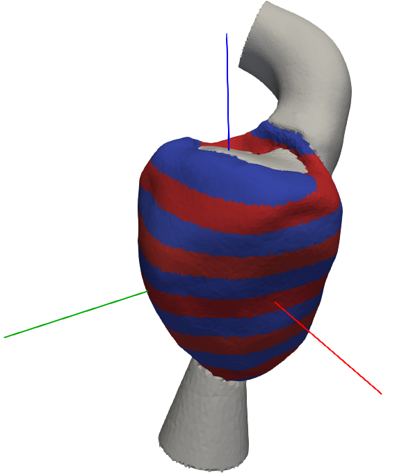 Figure 1
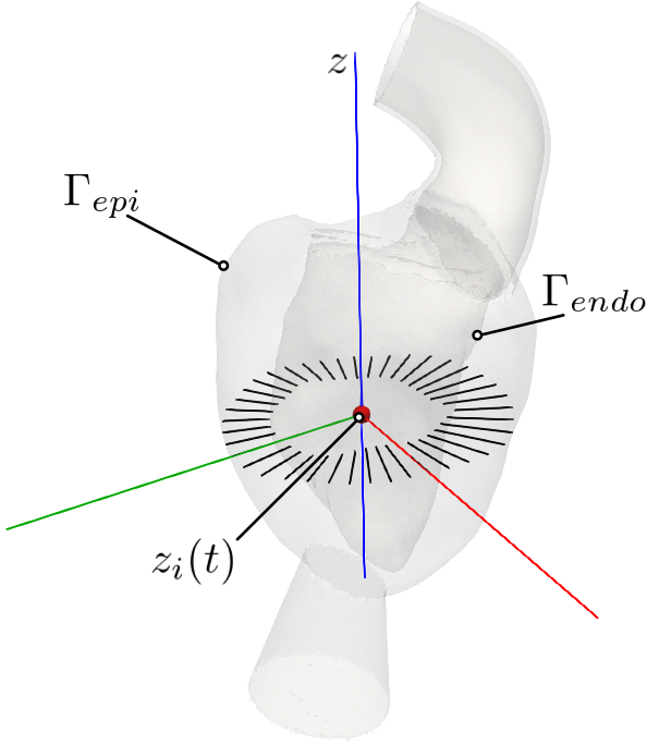 Figure 2
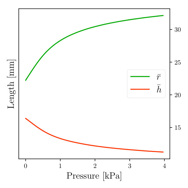 Figure 3
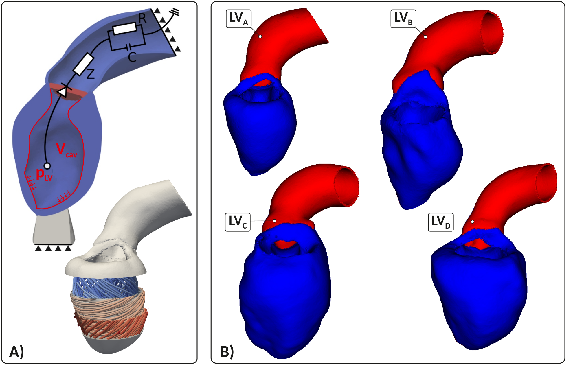 Figure 4
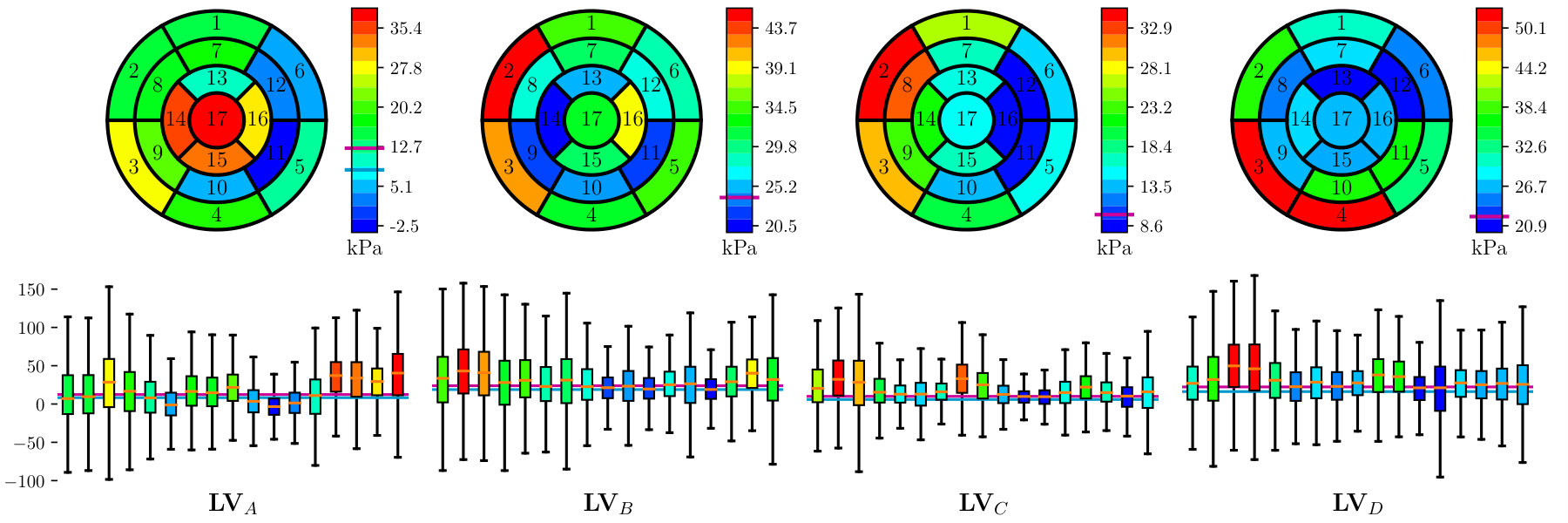 Figure 5
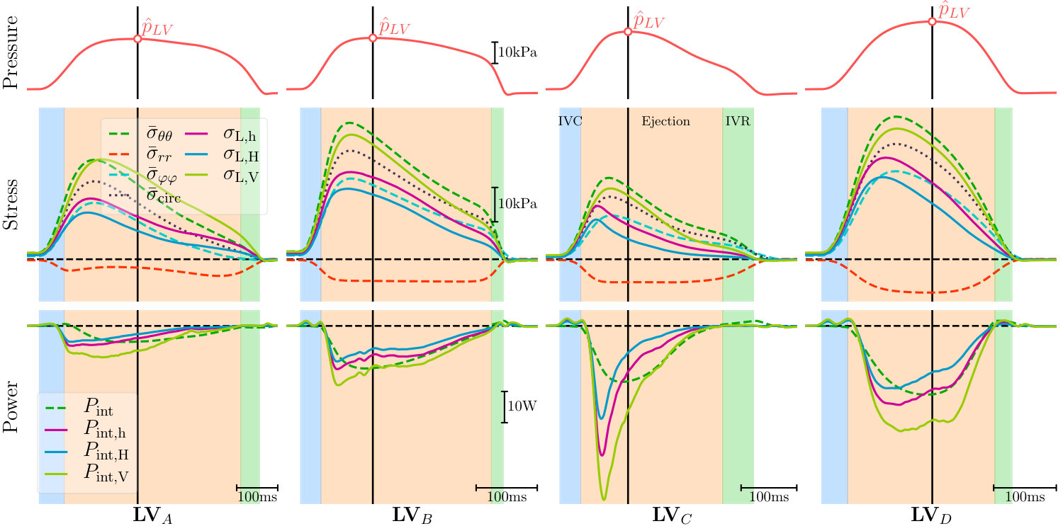 Figure 6
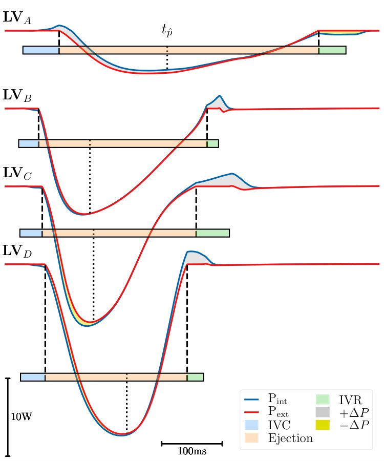 Figure 7
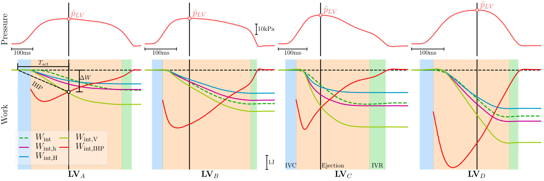 Figure 8
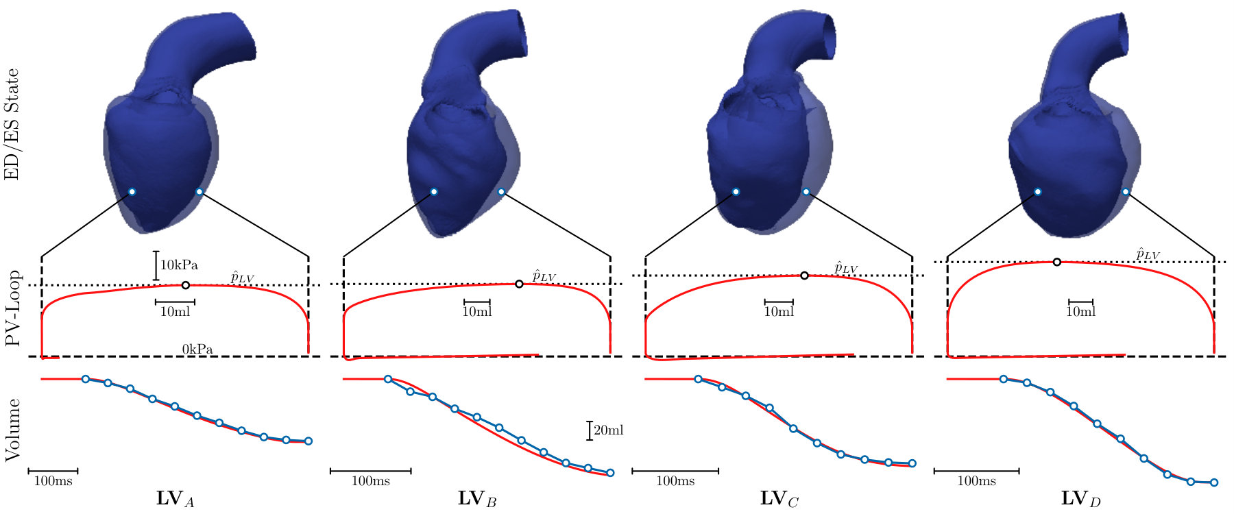 Figure 9
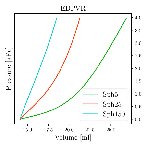 Figure 10
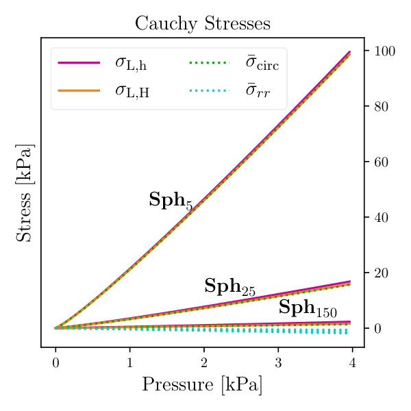 Figure 11
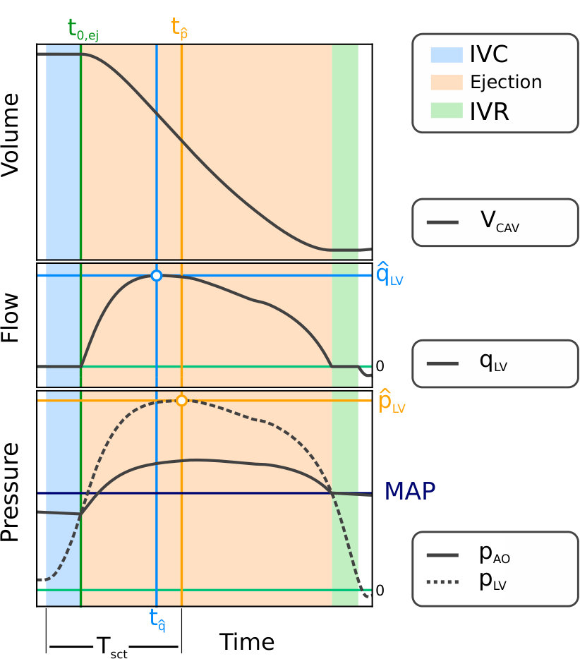 Figure 12
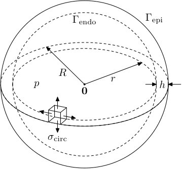 Figure 13
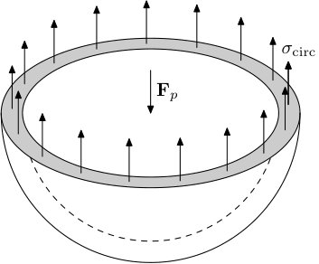 Figure 14
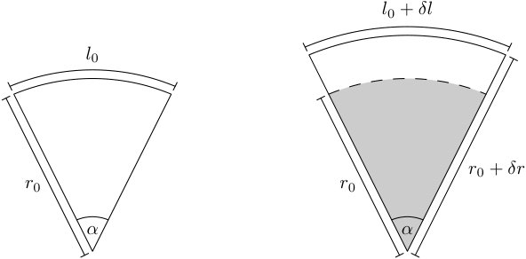 Figure 15
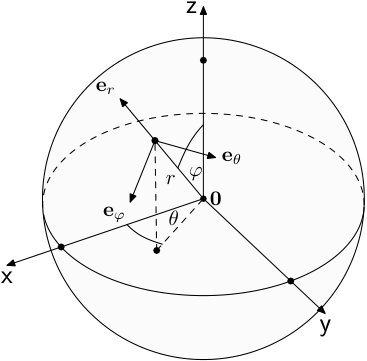 Figure 16
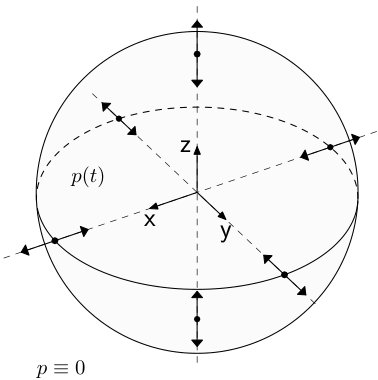 Figure 17
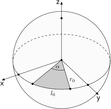 Figure 18
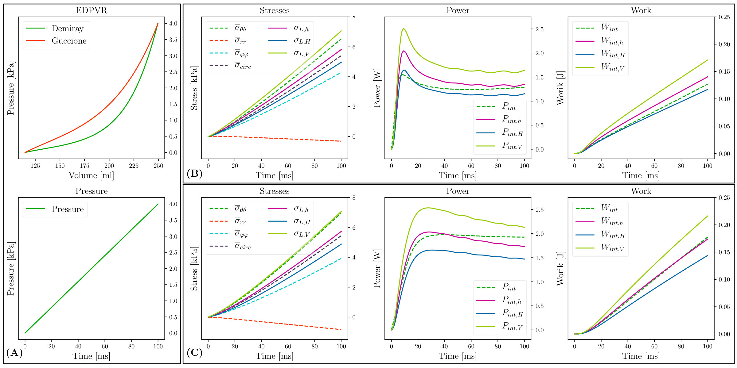 Figure 19
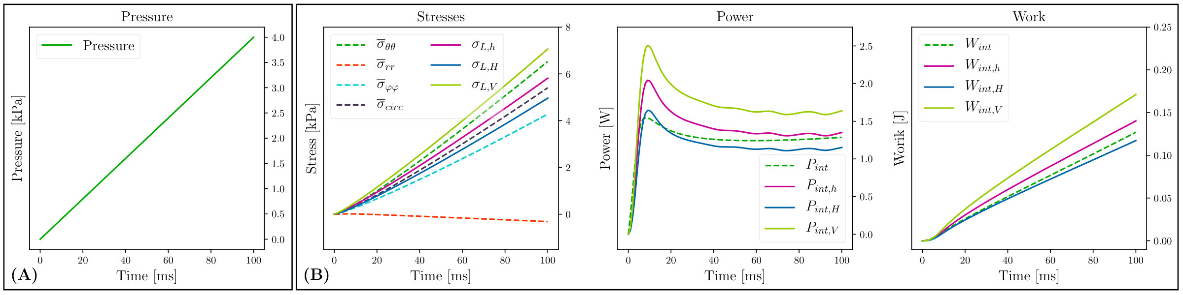 Figure 20
| Sex | Age | EDV | ESV | SV | EF | HR | MAP | HT | MVR | |||||
|---|---|---|---|---|---|---|---|---|---|---|---|---|---|---|
| [years] | [ml] | [ml] | [ml] | [%] | [min | [mmHg] | [mmHg] | [mmHg] | [mm] | [mmHg] | ||||
| A | F | No | No | |||||||||||
| B | M | No | Mild | |||||||||||
| C | M | Yes | Mild | |||||||||||
| D | M | Yes | No |
| [mm] | [mm] | [mm] | ||
|---|---|---|---|---|
| / / / |
| afterload | active stress | passive mechanical model | |||||
|---|---|---|---|---|---|---|---|
| [kPa] | [ms] | [kPa] | |||||
| Setup | [kPa] | [kPa] | [kPa] | [kPa] | [kPa] | [kPa] | #elements | [mm] |
|---|---|---|---|---|---|---|---|---|
| IHP | EHP | |||||||||||
|---|---|---|---|---|---|---|---|---|---|---|---|---|
| [W] | [W] | [W] | [W] | [W] | [W] | [W] | [W] | [W] | [W] | [1] | [1] | |
| Setup | [kPa] | [kPa] | [kPa] | [kPa] | [kPa] | [kPa] | #elements | [mm] |
|---|---|---|---|---|---|---|---|---|
| Setup | [mJ] | [mJ] | [mJ] | [mJ] | [mJ] | #elements | [mm] |
Peer Reviews
No public reviews on file for this paper yet. If you reviewed it on a platform where reviews are public (OpenReview, ICLR, NeurIPS, ICML), you can paste yours below so the community can read it here.
Videos
No videos yet. Explain this paper in a talk, walkthrough, or lecture? Add one.
Assessment of wall stresses and mechanical heart power in the left ventricle:
Finite element modeling versus Laplace analysis ††thanks: This research was supported by the grants F3210-N18 and I2760-B30 from the Austrian Science Fund (FWF) and the EU grant CardioProof 611232 and a Marie Skłodowska–Curie fellowship (GA 750835) to CA.
Matthias A.F. Gsell
Institute of Biophysics, Medical University of Graz, Graz, Austria
Christoph M. Augustin
Institute of Biophysics, Medical University of Graz, Graz, Austria
Shadden Research Group, Department of Mechanical Engineering, University of California, Berkeley, CA, USA
Anton J. Prassl
Institute of Biophysics, Medical University of Graz, Graz, Austria
Elias Karabelas
Institute of Biophysics, Medical University of Graz, Graz, Austria
Joao F. Fernandes
Institute for Imaging Science and Computational Modelling in Cardiovascular Medicine, Charité-Universitätsmedizin Berlin, Berlin, Germany
Marcus Kelm
Department of Congenital Heart Disease/Pediatric Cardiology, German Heart Institute Berlin, Berlin, Germany
Institute for Imaging Science and Computational Modelling in Cardiovascular Medicine, Charité-Universitätsmedizin Berlin, Berlin, Germany
Leonid Goubergrits
Institute for Imaging Science and Computational Modelling in Cardiovascular Medicine, Charité-Universitätsmedizin Berlin, Berlin, Germany
Titus Kuehne
Department of Congenital Heart Disease/Pediatric Cardiology, German Heart Institute Berlin, Berlin, Germany
Institute for Imaging Science and Computational Modelling in Cardiovascular Medicine, Charité-Universitätsmedizin Berlin, Berlin, Germany
Gernot Plank
Institute of Biophysics, Medical University of Graz, Graz, Austria
Abstract
Introduction: Stenotic aortic valve disease (AS) causes pressure overload of the left ventricle (LV) that may trigger adverse remodeling and precipitate progression towards heart failure (HF). As myocardial energetics can be impaired during AS, LV wall stresses and biomechanical power provide a complementary view of LV performance that may aide in better assessing the state of disease. Objectives: Using a high-resolution electro-mechanical (EM) in silico model of the LV as a reference, we evaluated clinically feasible Laplace-based methods for assessing global LV wall stresses and biomechanical power. Methods: We used in silico finite element (FE) EM models of LV and aorta of patients suffering from AS. All models were personalized with clinical data under pre-treatment conditions. LV wall stresses and biomechanical power were computed accurately from FE kinematic data and compared to Laplace-based estimation methods which were applied to the same FE model data. Results and Conclusion: Laplace estimates of LV wall stress are able to provide a rough approximation of global mean stress in the circumferential-longitudinal plane of the LV. However, according to FE results spatial heterogeneity of stresses in the LV wall is significant, leading to major discrepancies between local stresses and global mean stress. Assessment of mechanical power with Laplace methods is feasible, but these are inferior in accuracy compared to FE models. The accurate assessment of stress and power density distribution in the LV wall is only feasible based on patient-specific FE modeling.
Keywords: Aortic stenosis, transvalvular pressure gradient, heart failure
00footnotetext: Abbreviations: AVD, aortic valve disease; LV, left ventricle; HF, heart failure; PV, pressure-volume; EM, electro-mechanical; IHP, internal mechanical heart power; FE, finite element; IVC, isovolumetric contraction; IVR, isovolumetric relaxation.
1 Introduction
In AS elevated pressure gradients impose a higher load upon the LV. Under such conditions, the pressure produced by the LV must increase in order to achieve an adequate cardiac output that meets the metabolic demands. This requires the LV wall to generate higher active forces, which can be achieved either by an increase in wall stresses or a change in ventricular shape and mass. Such pressure overload conditions, if persistent for long enough, trigger adverse remodeling processes, eventually precipitating progression towards HF [17]. Treatments aim at alleviating pressure overload by reducing transvalvular pressure gradients closer to normal levels by surgical or catheter based aortic valve replacement [3]. However, re-stenosis frequently occurs and despite a successful reduction of transvalvular pressure gradients, a majority of patients remains hypertensive, consequently showing increased risk for irreversible course of HF and higher morbidity and mortality [14]. Thus, a successful reduction of pathologically elevated pressure gradients alone cannot be considered a reliable prognostic marker of long-term post-treatment outcomes in these patient cohorts.
As a consequence, alternative biomarkers beyond pressure gradients are sought to that provide a complementary view of cardiac function and, potentially, offer a higher predictive power with regard to outcomes. In a recent study, the use of end-diastolic or end-systolic wall stresses as assessed by a wall stress index has been proposed as a novel diagnostic criterion of HF [4]. This is physiologically motivated as elevated wall stress levels are assumed to impair the balance between metabolic supply and demand [36] by hindering perfusion and, thus, contribute towards adverse remodeling [1]. Wall stresses are directly linked to the mechanical power generated by the myocardial muscle and the work performed by it and as such can be considered a metabolic marker. Different approaches have been proposed to assess work and the energy expenditure of the myocardium. As a direct measurement of energy metabolism Positron Emission Tomography (PET) was used [19, 20], however the method is limited due to its complexity including the need for tracers involving ionizing radiation. More recently, a concept of biomechanical internal myocardial heart power (IHP), necessary to maintain adequate cardiac output (EHP, external heart power), has been introduced in patients with aortic coarctation [15]. Findings in this cohort suggest that the ratio , referred to as power efficiency, improved mostly in those cases with elevated IHP. While potential marker qualities of such concepts need to be further evaluated, it has remained a yearned-for goal to lower energy expenditure and increase efficiency of the myocardium likewise in any treatment procedure, including those for stenotic valvular and vascular disease.
Another method used to determine the work performed by the muscle is pressure-volume (PV) relations. These are usually measured using conductance catheter techniques. However, these procedures are invasive, time-consuming and expensive. Alternatively, PV-loops are measured with 3D echo or MRI [2], but even these methods are complex and pressure and volume traces are not recorded simultaneously.
Despite the diagnostic potential of markers based on wall stresses and expended mechanical power, this assessment has not evolved towards a routinely used diagnostic tool in the clinic mainly due to methodological limitations. Attempts to address this relied upon different variants of Laplace’s law, which require the acquisition of only a small number of measures representing LV cavity volume, wall width and pressure [4, 15]. However, these approaches are based on simplifications with regard to LV geometry, tissue structure and biomechanical properties as they assume the LV a thin-walled mechanically isotropic spherical shell. The accuracy and validity of these simplifications have not been firmly established, thus casting doubt on the reliability and fidelity of any metrics based on them [27, 41]. Experimental validation based on direct measurements of stresses in vivo is challenging and not feasible yet with currently available technologies. However, an indirect inference is viable using computational tools such as FE modeling where 3D wall stresses can be computed from a set of reliable strains – either measured in vivo [5, 23] or computed in silico [7] – using constitutive material models which are derived from ex vivo measurements [18] and material parameters fitted to clinical data [7, 40].
To evaluate the accuracy of Laplace analysis for estimating global wall stresses and mechanical power in the LV we employed four FE based EM LV models which have been previously fitted and validated with clinical data [7] under pre-treatment conditions. These models provide reliable strain data at a high spatio-temporal resolution from which wall stresses, biomechanical power and work in the LV can be determined at the best possible accuracy. Laplace analysis was applied to these in silico models to estimate hoop stress and mechanical power over a cardiac cycle and compared to the global ground truth data based on FE analysis.
2 Methods
2.1 Patient Data
Data from four AS patients with clinical indication for aortic valve treatment, all preceding a cardiac magnetic resonance study, were used (Tab. 1). AS treatment indicators included valve area and/or systolic pressure drop across the valve. The study was approved by the institutional Research Ethics Committee following the ethical guidelines of the 1975 Declaration of Helsinki. Written informed consent was obtained from the participants’ guardians.
2.2 Biomechanical FE model
The ventricular myocardium was modeled as a non-linear, hyperelastic, nearly incompressible and anisotropic material with a layered organization of myocytes and fibres that is characterized by a right-handed orthonormal set of basis vectors [18, 22]. These basis vectors consist of the fiber axis , which coincides with the prevailing orientation of the myocytes at location , the sheet axis , and the sheet-normal axis . The mechanical deformation of the tissue is described by Cauchy’s equation of motion under stationary equilibrium assumptions leading to a quasi-static boundary value problem: for a given pressure , find the unknown displacement such that
[TABLE]
holds for . By we denote the deformed geometry and by we define its boundary with and . The normal outward vector of is denoted by . The total Cauchy stress tensor refers to the sum of a passive stress tensor and an active stress tensor . That is, with
[TABLE]
where is the deformation gradient, is the strain energy function, is fiber orientation in the reference configuration, is the Jacobian, is the right Cauchy–Green strain tensor and is the scalar active contractile stress generated by the myocytes acting along .
The passive behavior of myocardial tissue was modeled using two material models, either the transversely-isotropic Guccione et al. model [18],
[TABLE]
where
[TABLE]
and is the modified isochoric Green–Lagrange strain tensor, or the isotropic Demiray model [12]
[TABLE]
with the modified isochoric right Cauchy–Green tensor. In both models, Eqs. (4) and (6), the bulk modulus , which serves as a penalty parameter to enforce near incompressibility, was chosen as kPa.
A simplified phenomenological contractile model [31] was used to represent active stress generation:
[TABLE]
where is the peak isometric tension, is a non-linear function dependent on fiber stretch describing the length-dependence of active stress generation, is the onset of contraction, is the upstroke time constant, is the active stress transient duration and is the downstroke time constant. This simplified model allows efficient fitting to patient data as the parameters for peak stress, , and time constant of contraction, , and twitch duration, , are related to the two clinical key parameters of interest, peak pressure and maximum rate of pressure increase, in an intuitive manner.
Solving these equations under given mechanical boundary conditions using the FE method at a sufficiently high spatio-temporal discretization provides an accurate description of tissue kinematics. Computed displacement serve as input then in a post-processing procedure to evaluate wall stresses and to compute internal power expended by the LV (see Sec. 2.6).
A Newton scheme was applied in each time step to linearize the nonlinear boundary value problem (1) yielding a non-symmetric FE system. The linear FE system was solved by a parallel GMRES algorithm with an algebraic multigrid preconditioner. For the Newton scheme a relative tolerance of and an absolute tolerance of was used as stopping criterion.
2.3 Verification of finite element model
To verify the FE-based calculation of stress-derived metrics, a geometrically simple and well-studied benchmark problem was chosen for which circumferential hoop stresses can be found from Laplace’s law under the following assumptions:
- (A1)
The wall material is isotropic.
- (A2)
The shape is a symmetric spherical shell with inner radius, , and outer radius, .
- (A3)
The thickness of the wall, , is sufficiently small, that is, the wall thickness to radius of curvature ratio is small, .
Since all these assumptions are violated in the LV which is orthotropic (A1), non-spherical in shape (A2), and thick-walled (A3) with , differences between Laplace analysis and FE computation are to be expected. Three configurations were considered, an ideal thin-walled spherical shell, , which complies with all assumptions (A1)–(A3) and thus can serve as a reference for FE validation, and two thicker-walled spheres, and , where assumption (A3) is increasingly violated. Geometries and mechanical boundary conditions are illustrated in Fig. LABEL:sub@fig:sph:geom–LABEL:sub@fig:sph:bcs.
The inner radius was chosen as mm in all models with varying from mm to mm in and , respectively. The choices for are representative of the ratios found in the LVs of patients in this study (Tab. 2). In line with assumption (A1), the nonlinear isotropic material law stated in Eq. (6) was employed with kPa and . Passive inflation experiments were performed by solving (1) with and applying a pressure in the range from [math] to kPa to the endocardial surface, , which covers the range of pressures observed in vivo during diastole. Pressure at the epicardial surface, , was assumed to be zero. To render the solution of this pure Neumann problem unique, displacement boundary conditions were enforced at the intersections of the Cartesian axes with the epicardial surface by restricting displacements to the respective intersecting axes (see Fig LABEL:sub@fig:sph:bcs). Unstructured tetrahedral FE meshes were generated for the , and geometries where the mean spatial resolution, , was increased until solutions were deemed converged.
2.4 LV model
2.4.1 Anatomical Modeling
FE meshes of the LV anatomy and aortic root were generated from 3D whole heart MRI acquired at end diastole (ED) with mm resolution at the German Heart Center Berlin. Multi-label segmentation of the LV myocardium, LV cavity and aortic lumen was done using the ZIB Amira software (https://amira.zib.de/). Segmentations were smoothed and upsampled to a mm isotropic resolution [11]. The wall of the aorta was automatically generated by dilation of the aortic lumen with a thickness of mm, and the aorta was clipped before the branch of the brachiocephalic artery. Due to limited resolution valves were not segmented, but were included in the FE model as a thin layer of tissue for applying pressure boundary conditions and computation of cavity volume. The multi-label segmentations were meshed using CGAL (http://www.cgal.org/) with a target discretization of mm in the LV myocardium and mm in the aortic wall. For the transversely-isotropic Guccione material model, see Eq. (4), we equipped all models with a rule-based fiber architecture [9], where fibers rotated linearly from at the epicardium to at the endocardium (Fig. 2.A). All anatomical models built are shown in Fig. 2.
2.4.2 Model fitting
To remove rigid body motion and provide physiological boundary conditions that allow a vertical movement of the LV base, as observed in-vivo, mechanical boundary conditions were applied by fixing the terminal rim of the clipped aorta (Fig. 2.A) and resting the apex of the LV on an elastic cushion which was rigidly anchored at its base. Constitutive relations were represented by Eq. (4). Using the ED geometry, default material parameters and an estimated ED pressure (EDP), an initial guess of the stress-free reference configuration was computed by unloading the model using a backward displacement method [35, 10]. Since clinically recorded data of the ED PV-relation (EDPVR) are often limited, the Klotz relation [24] providing an empiric description of EDPVR, , was used as target to steer the fitting of constitutive parameters. In absence of accurate measurements of EDP we refrained from fitting all material parameters to . Rather, default values for the parameters , and were used as reported in the literature [18], and only the scaling parameter was adjusted individually for each patient. With a given data point (EDV,EDP) was fitted to minimize the difference in stress-free residual volume, , between model and Klotz curve. This yielded values for of , , and for the cases , , and , respectively.
A three-element Windkessel model of LV afterload was used to provide the pressure-flow relationship during ejection [39] (see Fig. 3). LV models were parameterized to match clinically recorded PV-data using LV cavity volume traces, , determined from Cine-MRI with a temporal resolution of , , and ms for , , and , respectively. Continuously monitored invasive pressure recordings were not available as catheterization was not indicated. Peak pressure in the LV was determined by estimating peak pressure in the aortic root from cuff pressure measurements and by determining the pressure drop at peak flow across the aortic valve from ultrasound flow measurements using Bernoulli’s law [13]. Windkessel parameters representing the aortic input impedance, , comprising the flow resistance of aortic valve, , and the characteristic input impedance of the aorta, , as well as resistance and compliance of the arterial system were fit to reproduce estimated LV peak pressure using measured volume traces as input.
In a final step, active mechanical properties were fit to the same hemodynamic data used for fitting the afterload model. A reaction-eikonal model was used to generate activation sequences and simulate action potential propagation in the LV [29]. Active stress generation was triggered with a prescribed electromechanical delay when the upstroke of the action potential crossed the mV threshold. Parameters peak stress, , time constant of contraction, , and twitch duration, , were adjusted manually to fit peak pressure, , duration of pressure pulse and flow. Due to the intuitive link of the active stress model given in Eq. (7) with the fitting targets, a satisfactory fit was achieved within 5 simulation runs. The goodness of fit was deemed sufficiently accurate when the clinically measured metrics EF, SV, MAP and peak LV pressure, , were matched within a margin of error of . Clinical input data and fitted model parameters are summarized in Tab. 3.
2.5 Myocardial wall stresses
Stresses can be computed from deformations using constitutive material models based on ex vivo experimental data which link stresses to strains. In the FE model stress tensors are computed by evaluating Eqs. (2) and (3), which yields a tensor where only 6 components are independent for symmetry reasons. For the models , and the stress tensor simplifies. Due to the assumption of isotropy in (A1) and symmetry in (A2), any solution, if expressed in a spherical coordinate system, must also be symmetric. Quantities computed in the FE Cartesian coordinate system are recast in spherical coordinates as defined in Fig. LABEL:sub@fig:sph:csys using a projection matrix, . For the total Cauchy stress tensor we obtain
[TABLE]
with the projection matrix and .
While all quantities in the spherical models must be perfectly symmetric this is not necessarily the case in the FE solutions. Depending on spatial resolution and boundary conditions, a minor numerical jitter around mean values will inevitably occur. For comparing FE with Laplace analysis averaged mean quantities were therefore computed over the entire domain by
[TABLE]
with being the FE solution at time and .
In a thin-walled spherical shell stresses in azimuthal and meridional direction must be equal due to symmetry, that is, , and with radial stresses can be assumed to be negligible relative to circumferential hoop stresses, that is, . The stress tensor in spherical coordinates simplifies therefore to
[TABLE]
As a reference for verifying FE-based stresses different variants of Laplace’s law were used. In particular, we use an extension of Laplace’s law which takes into account the finite thickness of the wall
[TABLE]
and refer to stress estimates based on this formula as Laplace stress in thick-walled spherical shells, . Exploiting assumption (A3), that is, and thus , allows a further simplification yielding
[TABLE]
which we refer to as Laplace stress in thin-walled spherical shells, . Finally, we consider a volume-based estimation of [26] defined as
[TABLE]
which has been used previously in clinical studies [4], We note that Eq. (13) is equivalent to Eq. (11) for a spherical shell. However, when applied to a non-spherical structure such as the LV this is not the case. Eq. (13) may offer advantages as the determination of and may be less ambiguous than the determination of a representative inner radius and wall thickness (see Sec. 2.8.1).
2.6 Myocardial power and work
For a given displacement at time , where refers to the duration of a cardiac cycle and marks the end of diastole, the biomechanical power density, , generated or consumed at location within the LV wall can be computed by evaluating
[TABLE]
where is the strain rate tensor and denotes the double contraction of two tensors, see e.g. [21] for further details. Integration of Eq. (14) over the entire myocardial wall yields the global biomechanical power, ,
[TABLE]
and integration of Eq. (15) over time yields an expression of biomechanical work, , performed
[TABLE]
Based on Laplace’s law biomechanical power can be estimated using
[TABLE]
where denotes which formula was used for estimating the circumferential wall stress that is, and approximates circumferential strains. For a derivation of Eq. (17) see supplementary material. Laplace-based mechanical work is estimated analogously to Eq. (16) yielding
[TABLE]
In addition, a recently introduced also Laplace-based relative power indicator, IHP, was evaluated which attempts to estimate the power generated by the LV around the instant of peak pressure, . Based on [32], the mechanical work expended, IHW, during contraction time, , defined as the time elapsed between the onset of isovolumetric contraction at and the instant of peak stress in the LV at , is approximated by
[TABLE]
IHW is interpreted as a measure of the mechanical potential energy stored in the LV from which a measure of the peak biomechanical power generated by the LV between and is derived then by
[TABLE]
Note that Eq. (20), in contrast to Eq. (17), does not include any measure of . Thus, while consistent in terms of physical units, IHP must be considered a relative indicator and not a physical measure of power.
2.7 Hydrodynamic power and work
Hydrodynamic power, , is given by
[TABLE]
where is the hydrostatic pressure acting at endocardial surface, and represents blood flow out of the LV cavity during ejection. Hydrodynamic work, , is then the work expended by the LV myocardium when changing the volume of its cavity, , given by
[TABLE]
or, equivalently, expressed as PV work by
[TABLE]
In absence of active stresses, i.e. , and isovolumetric contstraints imposed by valves upon , must hold. Under such conditions, external work can therefore serve as a reference for validating the FE-based computation of internal power and work. This is not necessarily the case during the isovolumetric phases of a heartbeat where internal work may be expended which does not necessarily manifest as external work. During these phases, changes in occur which may entail shape changes of the LV myocardium and thus induce a non-zero strain rate tensor . However, due to the isovlumetric constraints imposed by the incompressibility of the blood pool and the closed state of all valves, no global change in cavity volume can occur, i.e. .
Under healthy conditions, hydrodynamic power in the LV cavity equals the power delivered to the arterial system as transvalvular power losses are small. However, in AS cases where transvalvular pressure gradients, , are significant, the effective hydrodynamic power externally delivered to the arterial system is reduced. Following [15], we define external hydrodynamic heart power, EHP, as
[TABLE]
where MAP and CO are mean arterial pressure and cardiac output, respectively, and is the pressure in the aorta ascendens. Power efficiency, , has been defined previously in [15] as the ratio
[TABLE]
Since essentially relates the mean hydrodynamic power delivered to the arterial system to the peak biomechanical power generated by the LV myocardium during systole, can be expressed as
[TABLE]
where , and are determined based on Eqs. (15), (21) and (24), respectively. That is, can be estimated from hemodynamic data using or from LV deformation analysis using . Unlike in Eq. (25), which compares an absolute measure of external hydrodynamic power to a relative indicator of internal biomechanical peak power, Eq. (26) provides a physically consistent comparison.
2.8 Evaluation of Laplace-based assessment of wall stress and power
Human EM LV models which were validated against clinical data (see Sec. 2.4.2), provided accurate ground truth data on strains and stresses in the LV wall. Using these as reference, Laplace analysis was applied to the in silico models to assess its accuracy and validity.
2.8.1 Determination of clinical input data for Laplace-based analysis
Geometric input parameters and required for Laplace analysis must be determined from clinical imaging datasets. As LV shape deviates markedly from a spherical shell representative mean parameters of and must be found. Since there is no unique best solution to establish a geometric correspondence between LV shape and a spherical shell, various methods have been used in clinical applications. Typically, transverse slices from short-axis Cine-MRI scans were analyzed to measure, either manually or semi-automatically, and , where is measured in the postero-lateral wall, the septum or an average is taken. The analysis is either carried out in one representative mid-cavity LV short axis slice, or a number of slices is selected to capture representative basal, mid-cavity and apical LV cross-sections.
Similar issues arise when applying Laplace analysis to in silico datasets. In order to extract and as objectively as possible without operator bias, automated processing workflows were implemented (see Fig. 4). Analogous to the -slice selection in MRI protocols, the unstructured FE meshes of the LV models were decomposed into slices of mm resolution, comparable to the MRI out-of-plane resolution. Decomposition was achieved by first determining the long axis, , of the LV using principal component analysis (see Fig. LABEL:sub@fig:lv:slicing), which yielded, depending on the spatial extent of the LV long-axis of a given model, between and slices, each slice is centered around . A mean coordinate of the LV in its current configuration, , was computed to define the center slice plane using the long-axis unit vector, , and the center of individual slices was shifted, keeping slice width and distance to the LV center constant. Within a selected plane, radial vectors, , were computed that emanated from and were oriented in polar angles ranging from [math] to with an angular sampling of . For each vector , the intersection with surfaces, and , was determined, yielding inner radii, , outer radii, and wall widths, (Fig. LABEL:sub@fig:lv:slice_avg). Mean radius, , and wall width, , were determined as the arithmetic average
[TABLE]
Finally, multi-slice mean and were computed by averaging over slices
[TABLE]
The time course of the mean values and (see Fig. LABEL:sub@fig:lv:mean_r_h_of_t) was plugged then into the respective Laplace equations to compute stress in Eqs. (11), (12), and (13), power in Eq. (17) and work in Eq. (18).
2.8.2 Simulation protocols and data analysis
To evaluate the influence of violating the assumptions (A1) and (A2), passive inflation experiments were performed with LV models and the anisotropic material given in Eq. (4) following the same protocol as applied before to the spherical shell models , and in Sec. 2.3. Laplace-based stress estimates , and were compared to the mean stresses obtained from the FE solution. Stresses were evaluated with respect to an ellipsoidal coordinate system to facilitate a comparison with stresses in the spherical shell models (see Fig. LABEL:sub@fig:sph:csys). An ellipsoidal coordinate system was constructed for the LV models by assigning fiber and sheet orientations using a rule-based method with a constant fiber angle of [9]. Stress components , and were averaged according to Eq. (9) yielding , and , respectively. Laplace-based estimation of power, {{P}_{\text{int,\star}}}, was compared to FE-based power, , and to external hydrodynamic power in the LV cavity, .
Laplace analysis was applied to clinically fitted EM LV models – to compare LV stress {{\sigma}_{\text{L,\star}}}, power {{P}_{\text{int,\star}}} and IHP over an entire systolic cycle to the FE-based stresses , , and , and biomechanical power . Further, biomechanical power due to LV deformation, , and hydrodynamic power, , derived from PV data were also compared to assess differences during isovolumetric phases.
2.9 Numerical Solution
Discretization of all PDEs and the solution of the arising systems of equations relied upon the Cardiac Arrhythmia Research Package framework [37]. Details on FE discretization [33] as well as numerical solution of electrophysiology [38, 28, 29] and electro-mechanics [8] equations have been described in detail previously. Both electrophysiolgy and mechanics FE solvers were validated previously in N-version benchmark studies [30, 25].
3 Results
3.1 Verification of FE model
The FE implementation was verified by performing passive inflation experiments with spherical shell models for which Laplace laws are known to be almost exact () or, at least, sufficiently accurate ( and ). The resulting EDPVRs and principal components of the Cauchy stress , evaluated in spherical coordinates and globally averaged to yield mean stresses and , are shown in Figs. LABEL:sub@fig:_edpvr_sph and LABEL:sub@fig:_edpvr_stress. A numerical comparison of stresses and work at the maximum pressure of kPa is provided in Tab. 4 and Tab. 7 in the supplement.
Agreement of FE-based mean circumferential stress with Laplace laws was very close, that is, held. With increasing provided estimates that were closer to the FE-based stress than (Tab. 4). The simple Laplace overestimated in , and by , and whereas with deviations were much smaller with , and . Radial stresses were negligible in the thinner-walled models and , that is, , but not in the thick-walled model where amounted to of . A comparison of FE-based work to Laplace-based and is given in Tab. 7 in the supplement.
3.2 Evaluation of Laplace-based assessment of wall stresses and power
After verification with spherical shell models FE analysis was applied to a validated in silico EM LV model to compute stresses, power and work during both diastolic and systolic phases. Since all assumptions underlying Laplace laws are violated in LV models the FE-based results were considered the ground truth and, thus, could be used to gauge the accuracy of Laplace-based assessment of LV mechanics.
3.2.1 Passive inflation of LV models
LV models – were inflated following the same protocol as in Sec. 2.3 (see Fig. 6.A). The temporal evolution of FE- and Laplace-based stresses, power and work are shown in Fig. 6 for model . Minor quantitative differences to other models – were observed, but qualitatively the overall behavior was identical. Stresses at kPa are summarized in Tab. 4, incurred work is given in Tab. 7 in the supplement.
3.2.2 Analysis of LV cycle experiments
Using Cine-MRI-based LV volume traces and estimated as inputs the models – were fitted over the cycle phases isovolumetric contraction (IVC), ejection and isovolumetric relaxation (IVR) (Fig. 7). All models replicated the clinical metrics of interest such as SV, EF or peak aortic pressure with sufficient accuracy ().
Fig. 8 compares the time course of the averaged FE-based quantities azimuthal, meridionial, radial and circumferential mean stresses, , , and , respectively and power to the Laplace-based estimation of stresses {{\sigma}_{\text{L,\star}}} and power {{P}_{\text{int,\star}}}. In all cases, the Laplace-based stresses and tended to underestimate the FE-based mean circumferential stress , being closer to the azimuthal stress , whereas overestimated and was closer to . Further, both Laplace stresses or globally averaged mean stresses deviate noticeably from the true local stresses acting at a given location (Fig. 9).
Laplace-based power estimates , and were qualitatively comparable to the exact FE-based , but quantitatively marked discrepancies were observed. The time course of Laplace-based power showed both a faster onset and decay with an early peak in power. Quantitative differences between the Laplace estimates were also significant with . Around the instant deviations were in the range of , , and W for , , and , respectively. The relative IHP marker led to large deviations (see Fig. 13 in the supplement) from the true FE-based mechanical power, even around the instant of the IHP marker was intended for.
A numerical comparison between markers of LV peak power is given in Tab. 5. Differences between true mechanical peak power and at the instant of peak pressure, , were minor, with the maximum difference being W or . Laplace estimation of , evaluated at , misestimated by - . Interestingly, performed better than in all cases, but with non-negligible maximum relative errors of , , and for , , and , respectively. IHP overestimated significantly, in the range between to . Since the mechanical power developed during isovolumetric phases was marginal (see Fig. 14 in the supplement), the most accurate estimate of is obtained by computing from standard hemodynamic PV data. In terms of peak mechanical power the difference was less than or in all cases where can be estimated with high accuracy by taking the product of peak power and flow, .
4 Discussion
Wall stress and mechanical power generated by the LV are considered important biomarkers that promise potential clinical utility for diagnosis and as a predictor of post-treatment LV remodeling after interventions [4, 15]. Moreover, the modelling of stresses and power would allow to gain an improved understanding of mechanisms that contribute to adverse remodelling. Laplace analysis would have the charme that inputs such as , , , and are accessible within routine clinical procedures. However, Laplace analysis is based on a global force balance calculation and relies upon simplifying assumptions on LV shape, tissue structure and biomechanical behavior. This study attempts to establish validity, accuracy and potential limitations of Laplace analysis of stresses and mechanical power generated by the LV by comparing against a FE model for which these quantities can be determined with high accuracy.
4.1 FE verification
FE computation of stresses and mechanical power was verified by performing passive inflation experiments with geometrically well defined spherical shell models of varying wall width for which Laplace laws hold with sufficient accuracy. FE computed circumferential stresses in all models agreed closely with the Laplace stresses {{\sigma}_{\text{L,\star}}} (see Fig. 5 and Tab. 4). As expected, with increasing , deviations became more pronounced and the thick-walled Laplace stresses agreed closer with FE stresses than the standard Laplace stress . In terms of work expended, more noticeable discrepancies were observed between and Laplace-based {{W}_{\text{int,\star}}} (see Tab. 7 in the supplement). However, since the agreement between FE-computed internal work and external work was essentially perfect, as expected on grounds of conservation of energy, we concluded that our FE implementation for evaluating stresses, power and work is correct and that the observed deviations are rather attributable to inherent inaccuracies in the Laplace approximations. In particular, we consider the mean strain rate approximation in Eq. (17) and the omission of radial stresses likely candidate causes.
4.2 Laplace versus FE-based stress and power analysis
The validated high resolution in silico model served as a reference for evaluating the accuracy of the Laplace-based approximation of , and . While the FE models which were built from, fitted to and validated against clinical data, may deviate from clinical data within the limits of clinical data uncertainty, for assessing Laplace analysis, the FE model represents the ground truth as it provides accurate data on stresses and strains which can serve to compute local power and work densities and , respectively, as well as global , and with highest possible accuracy. All input parameters needed for Laplace analysis can be derived from the FE model with higher accuracy than what is achievable clinically. In this regard, the application of Laplace analysis to the in silico model can be considered a best case scenario.
4.2.1 Wall stress in the LV
Wall stress in the LV is a tensorial quantity that varies in space (see Fig. 9). The tensor comprises six independent components whereas Laplace stresses {{\sigma}_{\text{L,\star}}} provide only one scalar stress value representing a global circumferential or hoop stress, . While is equivalent to and in a thin-walled spherical shell such as (see Tab. 4) this is not the case in the LV as there is no direct equivalence to any component of . As shown in a FE modeling study by Zhang et al. [41], the correlation of Laplace stresses to fiber and cross-fiber stresses is poor. Conceptually, the force balance consideration used in the derivation of Laplace laws suggests that Laplace stresses are most likely representative of the mean stresses in the longitudinal-circumferential plane, . Indeed, a fair qualitative agreement was observed between and {{\sigma}_{\text{L,\star}}} during passive LV inflation as illustrated in Fig. 6. During ejection the time course of {{\sigma}_{\text{L,\star}}}(t) followed a similar trend as although waveforms deviated to different degrees owing to the marked differences in the LV anatomies. However, quantitatively discrepancies were significant during both passive inflation and over a LV cycle as evident in Fig. 6.B and in the stress panels of Fig. 8 with substantial differences in stress magnitudes between the various Laplace laws and the global circumferential mean stress with .
Besides the fundamental problem of stress heterogeneity and tensorial properties of LV wall stress, Laplace calculations are afflicted with significant uncertainties. The meaning of geometric parameters and required for the evaluation of Eqs. (11) or (12) is ambiguous when applied to the LV which deviates in shape markedly from a spherical shell. Therefore, and must be determined from averaging over a number of short axis Cine MRI scans to find representative values. Due to longitudinal shortening additional averaging occurs as different slices of the heart are being imaged during ejection. Thus, the determination of parameters and cannot be unique as the particular method employed for averaging, such as the one described in Eq. (28), influences, to some extent, the results. Using Eq. (13) seems to circumvent this problem since and are used as inputs which may be determined uniquely for the LV. However, in our simulations led to larger misestimations than and .
It is well known that Laplace-based calculation of stresses is afflicted with various inaccuracies [27]. Nonetheless, Laplace-based calculation of LV wall stresses has been used in clinical studies as a diagnostic criterion [4]. However, according to observations in this study based on an in silico model and in line with other studies [41], the scope for clinical applications appears narrow. Laplace stresses may provide information of diagnostic value, but, if so, rather as an empirical than a mechanistic marker. As a biomarker representing LV wall stresses in a physical sense Laplace-based calculations suffer from severe fundamental limitations.
4.2.2 Mechanical heart power and power efficiency
Mechanical heart power and cardiac power efficiency defined as the ratio between peak mechanical power expended by the LV, , and the mean hydrodynamic power delivered to the arterial system, EHP, have been proposed recently as a diagnostic marker [15]. On grounds of conservation of energy the global mechanical power expended by the LV and the hydrodynamic power transferred to the LV blood pool, , must be equal. Discrepancies may occur due to isovolumetric phases during which hydrodynamic power is close to zero, but mechanical power is expended by the LV to some extent as conformational changes of the LV myocardium and the shape of the LV cavity occur. However, in all models studied during isovolumetric phases was negligible (see Fig. 14 in the supplement). This does not conflict with experimental studies providing evidence of heterogeneous circumferential strains, longitudinal shortening and wall thickening during IVC [6]. Qualitatively similar behavior is observed in our in silico models, but magnitude and velocity of strain development is much smaller during IVC than during ejection. Thus, the strain rate tensors remained small during IVC and mechanical power expenditure was minor. In all LV models under study global mechanical power and the hydrodynamic power in the LV cavity were virtually identical (see Tab. 5 and Fig. 14 in the supplement). Hence, mechanical heart power can be determined either by analyzing the deformation of the LV myocardium or from PV relations in the LV.
The estimation of is feasible directly from LV deformation either by using FE models or, as suggested in [15], based on Laplace’s law where the latter approach is more readily applicable in the clinic. However, when global LV power is of interest, Laplace-based approaches do not seem to offer any additional benefits over more standard approaches relying on hemodynamic data for a number of reasons.
First of all, the evaluation of {{P}_{\text{int,\star}}} based on Eq. (17) introduces a systematic error which leads to a misestimation of the actual , even in the spherical shell models, since any work expended in the radial direction is ignored. Laplace’s law takes into account only circumferential stresses and neglects any radial stresses. As shown in Fig. 5, this simplification is only well justified in thin-walled structures such as , but introduces pronounced discrepancies for increased (see passive inflation experiments in Tab. 4 and Tab. 6 in the supplement as well as traces in Fig. 8). Secondly, in addition to the parameters needed for wall stress estimation which are afflicted with substantial uncertainties as discussed above, the parameters and are required. Using the approximation given by Eq. (37) in the supplement the estimation of requires that both inner and outer radii and of the LV can be tracked with sufficient temporal resolution and accuracy. However, as evidenced in Fig. 8, even when evaluated in an in silico model where tracking of these quantities is feasible with the highest possible accuracy, the overall accuracy of the method is rather poor with significant under- or overestimation of the true , depending on whether , or is used and whether an early or late phase of ejection is considered (see Fig. 8).
The evaluation of cardiac power efficiency or requires only point estimates of peak mechanical power.
Following [15], this is feasible by assuming that occurs at the instant of peak pressure, . Consistent with expectations based on Laplace’s law this was not the case in any of our LV models. As peak pressure and peak stress would only coincide under isometric conditions. In the contracting LV during ejection, the ratio decreases, thus facilitating a further increase of beyond the instant of peak pressure (see pressure and stress panels in Fig. 8). Nonetheless, the instants of peak power and peak pressure fell sufficiently close together with of , , and ms for , , and , respectively. Indeed, inspection of Tab. 5 and the power panels in Fig. 8 suggests that the Laplace-based estimation of seems feasible by evaluating power at the instant of peak pressure (compare , , , and in Tab. 5), albeit with inferior accuracy compared to estimations based on hemodynamic PV data.
Alternatively, the simpler marker can be used as in [15] which relies on IHP and does not require an estimation of . While simpler, its use brings about a number of drawbacks. Since is ignored IHP is only a relative marker that is non-linearly related to . Therefore, IHP provided highly inconsistent relative estimates of with errors varying in the range from to (see Tab. 5). Thus, IHP as an indicator of appears to be of insufficient accuracy even for clinical applications of modest accuracy demands. Overall, the scope for Laplace-based power estimation as proposed in [15] seems limited as standard methods based on hemodynamic data are afflicted with less uncertainty, offer higher accuracy and are easier to evaluate. As shown in Tab. 5, is straight forwardly approximated – with higher accuracy than any Laplace-based method – as the product of peak pressure and flow, .
The mechanical power generated by the LV is an indicator of metabolic demands. Local wall stresses and power densities governing energetic demand and supply ratios in the LV myocardium are known to play important roles as drivers of remodeling in the pressure-overloaded LV of AS patients. However, analogous to the stresses shown in Fig. 8 the distribution of power density in the LV wall is highly heterogeneous as well with significant regional variability around the global mean power density. In this view Laplace-based global markers derived from mechanical deformation such as or {{P}_{\text{int,\star}}} are not representative of local stresses and power within the LV myocardium and appear to offer limited insight and predictive power beyond standard PV analysis.
An accurate representation of local mechanical stresses and power over a cardiac cycle depends on reliable sets of strains . While techniques for measuring strains in 3D throughout the LV myocardium are available [23], such recordings are not part of clinical routine, their analysis requires expensive non-trivial post-processing and spatio-temporal resolution and accuracy are limited. A carefully fitted and validated FE-based EM LV model which replicates a patients physiology in terms of PV relations as well as LV kinematics, provides accurate data on strains at a high spatio-temporal resolution. Using an appropriate parameterized patient-specific constitutive model such as given in Eq. (4), can be used to compute LV wall stresses and or any other stress-related biomarker efficiently with high accuracy. Such models are able to provide either global power , but also fine-grained distributed power density . A spatio-temporal view on , and in the LV may provide additional insights as regions of elevated strain, stress or power are assumed to be implicated in the mechanisms driving remodeling in the pressure overloaded LV [16, 34].
5 Conclusions
Laplace estimates of LV wall stress are able to provide a rough approximation of global mean stress in the circumferential-longitudinal plane of the LV. However, according to FE results spatial heterogeneity of stresses in the LV wall is significant, leading to major discrepancies between local stresses and global mean stress. Assessment of mechanical power with Laplace methods is feasible, but these are inferior in accuracy compared to FE models and do not offer any benefits compared to standard methods based on hemodynamic data. In this view, the scope for Laplace-based analysis in clinical applications seems narrow. The accurate assessment of stress and power density distribution in the LV wall is only feasible based on patient-specific FE modeling.
6 Supplementary Material
6.1 Derivation of Laplace’s law
To derive the law of Laplace we consider a spherical shell of inner radius, and thin walls of a given thickness, . Inflating the shell by applying a pressure, , within the shell’s cavity, induces deformation which causes the buildup of stresses within the wall. If we consider one half of the sphere, the total force acting on the inner surface must be balanced with the total force acting over the cut surface (see Fig. LABEL:sub@supp:fig:sph:bof). Due to spherical symmetry, the circumferential stresses at any radius must be the same and the shear stress is zero. Integrating circumferential stresses over the cut surface yields the total force balancing the force due to the applied pressure. That is, we have
[TABLE]
Assuming that , radial stresses are small compared to circumferential stresses, , and the total stress tensor is approximated by
[TABLE]
with respect to the spherical coordinate system and the projection matrix , see Fig. LABEL:sub@supp:fig:sph:csys. Note that in a spherical shell differs from a stress tensor in the LV in various ways. Unlike in the LV, stresses in circumferential and meridonial/longitudinal direction are equal whereas in the LV longitudinal stresses tend to be larger than circumferential stresses. Further, the assumption is not justified, rather holds. Thus radial stresses in the LV are non-negligible, that is, is at an order of magnitude comparable to .
6.1.1 Laplace’s law for a thick-walled sphere
From Eq. (29) the circumferential stress in a thick-walled sphere is found as
[TABLE]
which we denote as .
6.1.2 Laplace’s law for a thin-walled sphere
Using assumption (A3), i.e. , we have which yields the simple law of Laplace for a thin-walled sphere given by
[TABLE]
which we denote as .
6.1.3 Volume-based stress
Since radius and wall thickness are two quantities which are not always available or are hard to determine for a general geometry like a LV, we rewrite Eq. (31) in terms of the cavity volume and the myocardial volume . For the spherical shell geometry there holds and which entails and . Using the volume-based representations of and , we can rewrite Eq. (31)
[TABLE]
which we denote as .
6.2 Computation of power and work
The approximations , and for the circumferential stress can be used to derive an estimator for the internal power
[TABLE]
and internal work
[TABLE]
For this sake, we consider Eq. (34) and the simplified representation of the total stress tensor Eq. 30. In Eq. (34) an approximation of the strain rate is required. Rewriting the strain tensor in spherical coordinates, as done for the stress tensor , we obtain
[TABLE]
where is the projection matrix introduced in Sec. 6.1. Similarly, the strain rate is expressed as
[TABLE]
Using Eq. (30), an approximation of the internal power density, can be derived as . Due to the assumption of symmetry (A2), strains in circumferential direction do not vary with space, i,e. , and the approximation for the internal power density simplifies to
[TABLE]
An approximation of the circumferential strain can be found based the Cauchy strain and considerations illustrated in Fig. 11. Accordingly, for a given radius circumferential strain can be approximated as
[TABLE]
and for the circumferential strain rate we obtain .
To approximate the circumferential strain rate of a spherical shell of thickness , we take the arithmetic mean of the strain rate at inner radius and outer radius , that is
[TABLE]
where is the initial inner radius and is the initial outer radius of the spherical shell at its stress free configuration, i.e. .
Using Eqs. (36) and (37), the internal power can be estimated by
[TABLE]
where is the volume of the shell’s wall at time .
Using an estimate for we obtain
[TABLE]
with and by integrating over time, we get an estimate for the internal work
[TABLE]
6.3 Methods
6.3.1 Model fitting
To delineate anisotropy from pure geometry effects, passive inflation experiments were also performed with LV models using the Demiray model and passive mechanical behavior was compared to the spherical shell models , and . In these cases, parameters were set to and was chosen in a patient-specific manner to obtain the same volume at maximum inflation pressure as with the Guccione model. Note that in none of the simulations of a full cardiac cycle the Demiray model was considered as the resulting kinematics was in stark contrast to the clinical data.
6.3.2 Analysis of LV inflation experiments
To evaluate the influence of violating the assumption on the geometry (A2), passive inflation experiments were performed with LV models and the isotropic material due to Demiray, Eq. (6), following the same protocol as applied to the spherical shell models , and . The parameter in the Demiray model was set to , , and kPa for the models , , and , respectively. The Laplace-based stress estimates , and were compared to the mean stresses obtained from the FE solution. Stresses were evaluated with respect to an ellipsoidal coordinate system to facilitate a comparison with stresses computed in the spherical shell models , and where spherical coordinates were used for stress analysis. The ellipsoidal coordinate system for the LV models was constructed by assigning fiber and sheet orientations using a rule-based method with a constant fiber angle of . Stress components , and were averaged yielding , and , respectively. Note that all models except showed marked spatial stress variations. Thus, the reported mean stresses may deviate considerably from the true local stresses . Laplace-based estimations of power {{P}_{\text{int,\star}}} and work {{W}_{\text{int,\star}}}, were compared to those obtained by FE simulation, and and to external hydrodynamic power and work in the LV cavity, and .
6.4 Results
6.4.1 Verification of the FE model
Similarly, with increasing the accuracy of the thick-walled Laplace estimate performed better than the simpler thin-walled Laplace estimate . As expected on grounds of conservation of energy, the agreement between biomechanical work and hemodynamic work was essentially perfect with differences for all models.
6.4.2 Passive inflation of LV models
The LV models – were inflated following the loading protocol in Fig. 12.A. Passive material behavior was represented compliant with (A1) by the isotropic Demiray model. The temporal evolution of FE- and Laplace-based stresses, power and work are shown in Fig. 12.B for model . Minor quantitative differences to other models – were observed, but qualitatively the overall behavior was identical. Stresses at kPa and the amount of work incurred during inflation up to this pressure are summarized in Tabs. 6 and 7.
6.4.3 Analysis of LV cycle experiments
The reference list from the paper itself. Each links out to its DOI / PubMed record.
- 1Aikawa et al. [2001] Y Aikawa, L Rohde, J Plehn, S C Greaves, F Menapace, M O Arnold, J L Rouleau, M A Pfeffer, R T Lee, and S D Solomon. Regional wall stress predicts ventricular remodeling after anteroseptal myocardial infarction in the healing and early afterload reducing trial (heart): an echocardiography-based structural analysis. American Heart Journal , 141:234–242, 2001.
- 2Al-Wakeel et al. [2016] Nadya Al-Wakeel, Katharina R Schmitt, Daniel R Messroghli, Eugénie Riesenkampff, Felix Berger, Titus Kuehne, Bjoern Peters, et al. Cardiac mri in patients with complex chd following primary or secondary implantation of mri-conditional pacemaker system. Cardiology in the Young , 26(2):306–314, 2016.
- 3Ali et al. [2018] Noman Ali, Peysh A Patel, and Steven J Lindsay. Recent developments and controversies in transcatheter aortic valve implantation. European Journal of Heart Failure , 2018.
- 4Alter et al. [2016] Peter Alter, A Rembert Koczulla, Christoph Nell, Jens H Figiel, Claus F Vogelmeier, and Marga B Rominger. Wall stress determines systolic and diastolic function–characteristics of heart failure. International Journal of Cardiology , 202:685–693, 2016.
- 5Ashikaga et al. [2007] Hiroshi Ashikaga, Benjamin A. Coppola, Bruce Hopenfeld, Eric S. Leifer, Elliot R. Mc Veigh, and Jeffrey H. Omens. Transmural dispersion of myofiber mechanics: implications for electrical heterogeneity in vivo. J Am Coll Cardiol , 49(8):909–916, 2007.
- 6Ashikaga et al. [2009] Hiroshi Ashikaga, Tycho I G van der Spoel, Benjamin A Coppola, and Jeffrey H Omens. Transmural myocardial mechanics during isovolumic contraction. JACC. Cardiovascular Imaging , 2:202–211, 2009.
- 7Augustin et al. [2016 a] Christoph M Augustin, Andrew Crozier, Aurel Neic, Anton J Prassl, Elias Karabelas, Tiago Ferreira da Silva, Joao F Fernandes, Fernando Campos, Titus Kuehne, and Gernot Plank. Patient-specific modeling of left ventricular electromechanics as a driver for haemodynamic analysis. Europace , 18:iv 121–iv 129, 2016 a.
- 8Augustin et al. [2016 b] Christoph M Augustin, Aurel Neic, Manfred Liebmann, Anton J Prassl, Steven A Niederer, Gundolf Haase, and Gernot Plank. Anatomically accurate high resolution modeling of human whole heart electromechanics: A strongly scalable algebraic multigrid solver method for nonlinear deformation. Journal of Computational Physics , 305:622–646, 2016 b.