A linear programming approach to the tracking of partials
Nicholas Esterer, Philippe Depalle

TL;DR
This paper introduces a linear programming method for tracking sinusoidal chirps that outperforms classical algorithms in noisy conditions and has lower complexity than existing approaches.
Contribution
It presents a novel LP formulation for sinusoidal partial tracking that improves efficiency and accuracy over traditional greedy and Viterbi-based methods.
Findings
LP approach outperforms classical algorithm in noisy environments
Complexity of LP method is less than previous approaches
LP method effectively tracks sinusoidal chirps in high noise levels
Abstract
A new approach to the tracking of sinusoidal chirps using linear programming is proposed. It is demonstrated that the classical algorithm of McAulay and Quatieri is greedy and exhibits exponential complexity for long searches, while approaches based on the Viterbi algorithm exhibit factorial complexity. A linear programming (LP) formulation to find the best paths in a lattice is described and its complexity is shown to be less than previous approaches. Finally it is demonstrated that the new LP formulation outperforms the classical algorithm in the tracking of sinusoidal chirps in high levels of noise.
Click any figure to enlarge with its caption.
 Figure 1
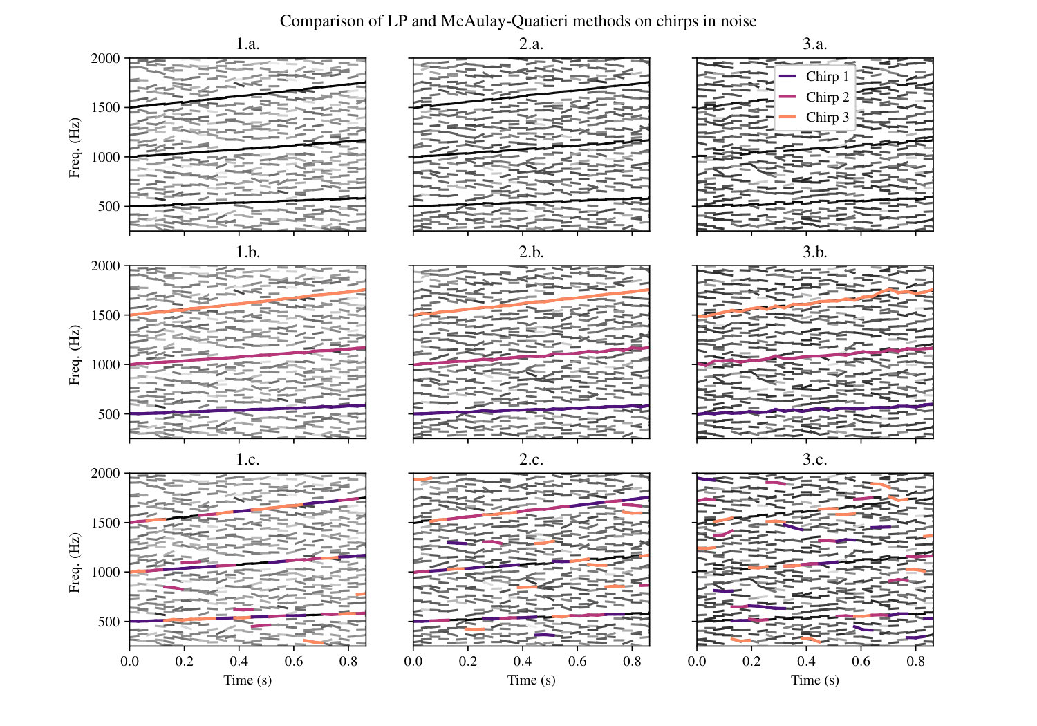 Figure 2
| 0 | 0 | 0.20 | 2.45 | 500 | 600 |
|---|---|---|---|---|---|
| 1 | 0 | 0.39 | 4.91 | 1000 | 1200 |
| 2 | 0 | 0.59 | 7.36 | 1500 | 1800 |
Peer Reviews
No public reviews on file for this paper yet. If you reviewed it on a platform where reviews are public (OpenReview, ICLR, NeurIPS, ICML), you can paste yours below so the community can read it here.
Videos
No videos yet. Explain this paper in a talk, walkthrough, or lecture? Add one.
Taxonomy
TopicsBlind Source Separation Techniques · Advanced Adaptive Filtering Techniques · Speech and Audio Processing
A linear programming approach to the tracking of partials
Abstract
A new approach to the tracking of sinusoidal chirps using linear programming is proposed. It is demonstrated that the classical algorithm of [mcaulay1986speech] is greedy and exhibits exponential complexity for long searches, while approaches based on the Viterbi algorithm exhibit factorial complexity [depalle1993tracking] [wolf1989finding]. A linear programming (LP) formulation to find the best paths in a lattice is described and its complexity is shown to be less than previous approaches. Finally it is demonstrated that the new LP formulation outperforms the classical algorithm in the tracking of sinusoidal chirps in high levels of noise.
Index Terms— partial tracking, linear programming, optimization, additive synthesis, atomic decomposition, regularized approximation
1 Introduction
Atomic decompositions of audio allow for the discovery of meaningful underlying structures such as musical notes [gribonval2003harmonic] or sparse representations [plumbley2010sparse]. A classical structure sought in decompositions of speech and music signals is the sum-of-sinusoids model: windowed sinusoidal atoms in the decomposition of sufficient energy and in close proximity in both time and frequency are considered as connected. The progressions of these connected atoms in time form paths or partial trajectories.
Many authors have considered the partial tracking problem, beginning with [mcaulay1986speech]. Their technique is improved upon in [lagrange2003enhanced] with the use of linear prediction to improve the plausibility of partial tracks. Rather than seeking individual paths, in [depalle1993tracking] the most plausible sequence of connections and detachments between atoms is determined via an extension of the Viterbi algorithm proposed in [wolf1989finding]. Improvements to this technique are made in [kereliuk2008improved] by incorporating the frequency slope into atom proximity evaluations.
The latter techniques seeking globally optimal sets of paths incur great computational cost due to the large number of possible solutions. For this reason, in this paper we propose a linear programming relaxation formulation of the optimal path-set problem based on an algorithm for the tracking of multiple objects in video [jiang2007linear]. It will be shown that this algorithm has favourable asymptotic complexity and performs well on the tracking of chirps in high levels of noise.
1.1 Note on notation
The atomic decompositions used in this paper consider blocks of of contiguous samples, called frames and these frames are computed every samples, being the hop-size. We will denote the sets of parameters for atoms found in the decomposition in frame as and the in frame as where and refer to adjacent frames.
The total number of nodes is . is the th node of the th frame, the set of all the nodes in the th frame and the th node out of all nodes ().
We are interested in paths that extend across frames where each path touches only one parameter set and each parameter set is either exclusive to a single path or is not on a path.
In this paper, indexing starts at 0. If we have a vector then is the th row or column of that vector depending on the orientation. The same notation is used for Cartesian products, e.g., if and are sets and then for the pair is the first item in the pair and the second.
2 A greedy method
In this section, we present the McAulay-Quatieri method of peak matching. It is conceptually simple and a set of short paths can be computed quickly, but it can be sensitive to spurious peaks and its complexity becomes unwieldly for long searches.
In [mcaulay1986speech, p. 748] the peak matching algorithm is described in a number of steps; we summarize them here in a way comparable with the linear programming formulation to be presented shortly. In that paper, the parameters of each data point are the instantaneous amplitude, phase, and frequency but here we allow for arbitrary parameter sets . Define a distance function that computes the similarity between sets of parameters. We will now consider a method that finds tuples of parameters that are closest.
We compute the cost tensor . For each , find the indices corresponding to the shortest distance, then remove the th rows (lines of table entries) in the their respective dimensions from consideration and continue until tuples have been determined or a distance between a pair of nodes on the path exceeds some threshold . This is summarized in Algorithm 1.
This is a greedy algorithm because on every iteration the smallest cost is identified and its indices are removed from consideration. Perhaps choosing a slightly higher cost in one iteration would allow smaller costs to be chosen in successive iterations. This algorithm does not allow for that. In other terms, the algorithm does not find a set of pairs that represent a globally minimal sum of costs. Furthermore, the algorithm does not scale well: assuming equal numbers of parameter sets in all frames, the search space grows exponentially with . Nevertheless, the method is simple to implement, computationally negligible when is small, and works well with a variety of audio signals such as speech [mcaulay1986speech] and music [smith1987parshl].
3 best paths through a lattice via linear programming (LP)
In this section we show how to find L paths through a lattice of frames such that the sets of nodes on each path are disjoint. The th frame of the lattice contains nodes for a total of nodes.
Similar to the McAulay-Quatieri method we define the cost as the limiting cost under which the connection between two nodes will be considered in the LP method.
The solution vector to the linear program shall indicate the presence of a connection between a pair of nodes by having an entry equal to and otherwise have entries equal to [math]. To enumerate the set of possible connection-pairs we define
[TABLE]
The cost vector of the objective function is then
[TABLE]
and the length of is , in other words, pairs of nodes. For convenience we define a bijective mapping giving the index in of the pair . For the implementation considered in this paper, for all not in adjacent frames and so will be no larger than (assuming the same number of nodes in each frame).
The total cost of the paths in the solution is then calculated through the inner product . To obtain that represents disjoint paths we must place constraints on the structure of the solution. Some of the constraints presented in the following are redundant but the redundancies are kept for clarity; later we will show which constraints can be removed without changing the optimal solution .
All nodes in will have at most one incoming connection or otherwise no connections, a constraint that can be enforced through the following linear inequality: define with , the number of nodes in all the frames excluding the first. We sum all the connections into the node represented by the respective entry in through an inner product with the th row in and require that this sum be between [math] and , i.e.,
[TABLE]
and
[TABLE]
Similarly, to constrain the number of outgoing connections into each node, we define and with
[TABLE]
and
[TABLE]
To forbid breaks in the paths it is required that the number of incoming connections into a given node equal the number of outgoing connections for the nodes potentially having both incoming and outgoing connections.
[TABLE]
and
[TABLE]
Finally we ensure that there are paths by counting the number of connections in each frame and constraining this sum to be . We choose arbitrarily to count the number of outgoing connections by summing rows of into rows of
[TABLE]
with and and
[TABLE]
As stated above, some of these constraints are redundant and can be removed. Indeed, we have , therefore we will always have and . Furthermore, all but the last row of (10) can be seen as constructed from linear combinations of rows of (8) and the last row of (10) so we only require . Finally we always have because of the constraint that there be a maximum of incoming and outgoing connection from each node.
The complete LP to find the best disjoint paths through a lattice described by node connections is then
[TABLE]
subject to
[TABLE]
[TABLE]
where is the identity matrix. A proof that the solution will have entries equal to either [math] or can be found in [parker1988discrete, p. 167].
4 Memory complexity
To simplify notation, in this section we assume there are nodes in each frame of the lattice.
Although the matrices involved in (11) are large, only a small fraction of their values are non-zero. Matrices , but each contains only non-zero entries. Furthermore but contains only non-zero entries while contains merely . The constraint requires a matrix with non-zero entries. The total memory complexity including the entries in and the right-hand-sides of (11) is non-zero floating-point numbers.
5 Complexity
Here we will compare the complexity of the LP formulation of the best paths search to the greedy McAulay-Quatieri method as well a combinatorial algorithm proposed in [wolf1989finding].
Assuming the same number of nodes in each frame of the lattice, the search for the th best path in the generalized McAulay-Quatieri algorithm () requires a search over possible paths.
The LP formulation of the -best paths problem gives results equivalent to the solution to the -best paths problem proposed in [wolf1989finding]. The complexity of the algorithm by Wolf in [wolf1989finding] is equivalent to the Viterbi algorithm for finding the single best path through a trellis whose th frame has connections where and are the number of nodes in two consecutive frames of the original lattice. Therefore, assuming a constant number of nodes in each frame, its complexity is .
The complexity of the algorithm presented here is polynomial in the number of variables (the size of ). Assuming we use the algorithm in [karmarkar1984new] to solve the LP, our program has a complexity of where is the number of bits used to represent each number in the input. However, this bound is conservative considering the reported complexity of modern algorithms.
For instance, the complexity of a log-barrier interior-point method is dominated by solving the system of equations
[TABLE]
some s of times [boyd2004convex, p. 590]. Each iteration then takes flops (floating-point operations) to solve (12) using a standard -decomposition [golub1996matrix, p. 98]. As is a diagonal matrix, if the number of nodes in each frame is for all frames, then will be a block-diagonal matrix made up of blocks . The system can then be solved in
[TABLE]
flops [boyd2004convex, p. 675]; this complexity is without exploiting the sparsity of nor the structure of — the product of some diagonal matrix with an unchanging symmetric matrix .
6 Partial paths on an example signal
We compare the greedy and LP based methods for peak matching on a synthetic signal. The signal is composed of chirps of constant amplitude, the th chirp at sample described by the equation
[TABLE]
The parameters for the chirps are presented in Table 6.