Optimal acceptance sampling for modules F and F1 of the European Measuring Instruments Directive
Cord A. M\"uller

TL;DR
This paper develops an optimized acceptance sampling scheme for modules F and F1 of the European Measuring Instruments Directive, reducing sample sizes while maintaining required statistical protection.
Contribution
It introduces a new sampling plan that is more efficient than ISO 2859-1, applicable to both large and finite lots, based on binomial and hypergeometric distributions.
Findings
Smaller sample sizes achieved compared to ISO 2859-1
Applicable to large and finite lots with full statistical protection
Enhanced economic efficiency of sampling plans
Abstract
Acceptance sampling plans offered by ISO 2859-1 are far from optimal under the conditions for statistical verification in modules F and F1 as prescribed by Annex II of the Measuring Instruments Directive (MID) 2014/32/EU, resulting in sample sizes that are larger than necessary. An optimised single-sampling scheme is derived, both for large lots using the binomial distribution and for finite-sized lots using the exact hypergeometric distribution, resulting in smaller sample sizes that are economically more efficient while offering the full statistical protection required by the MID.
Click any figure to enlarge with its caption.
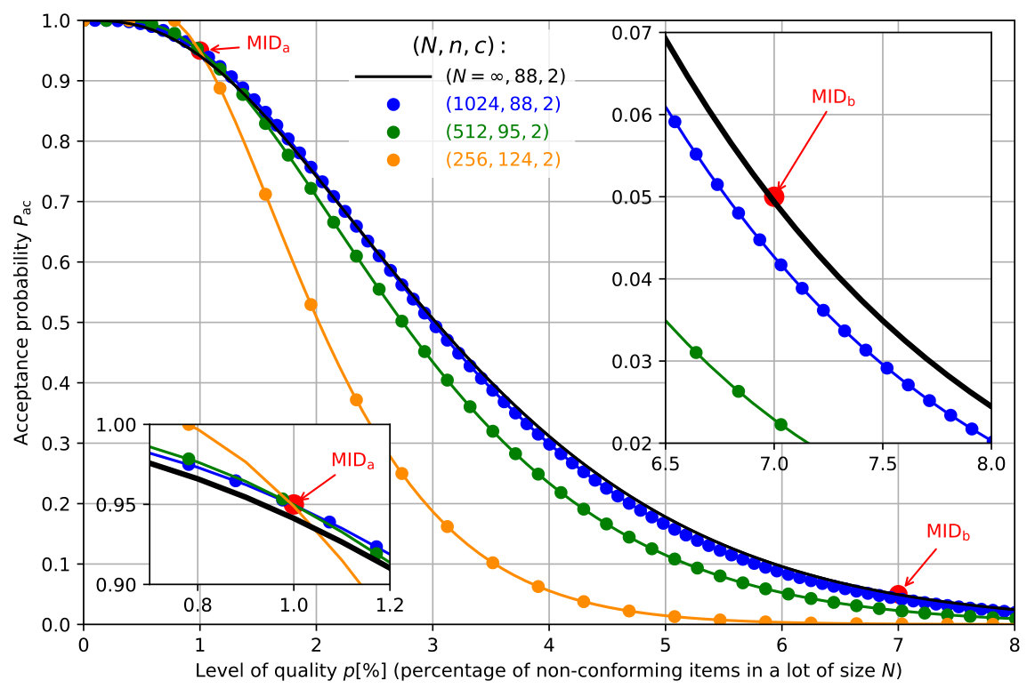 Figure 10
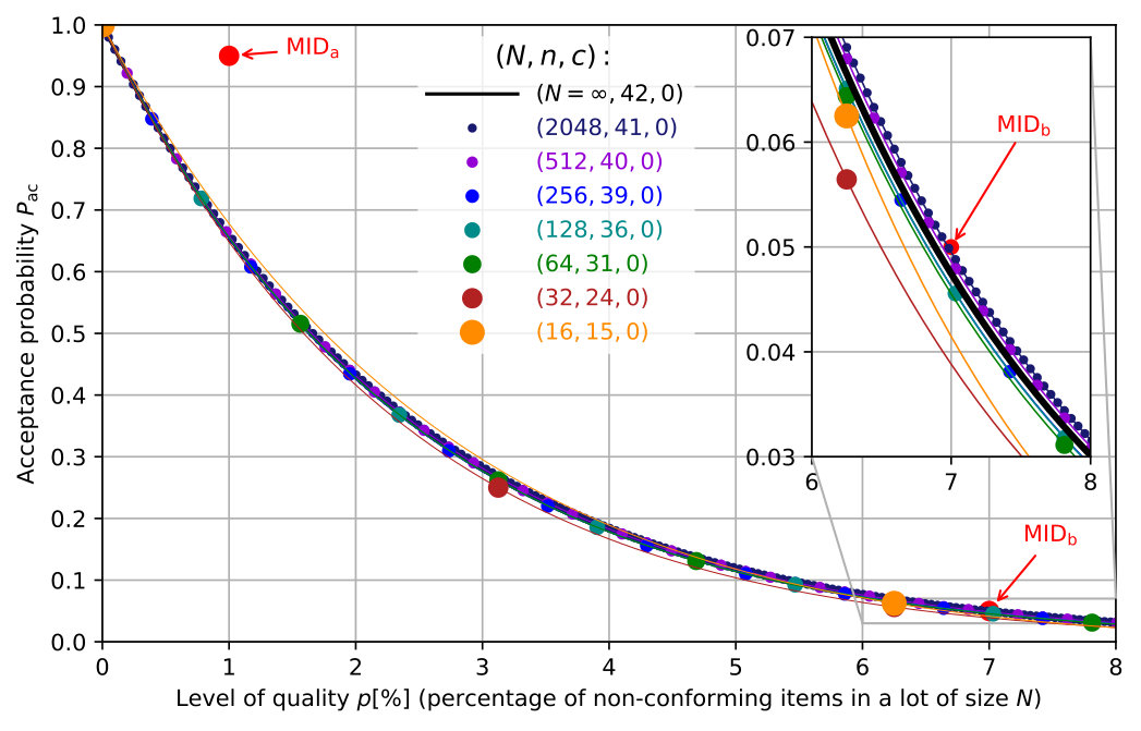 Figure 2
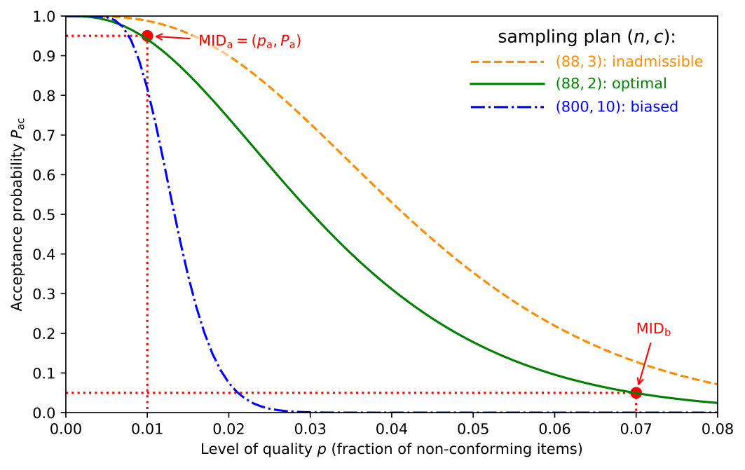 Figure 3
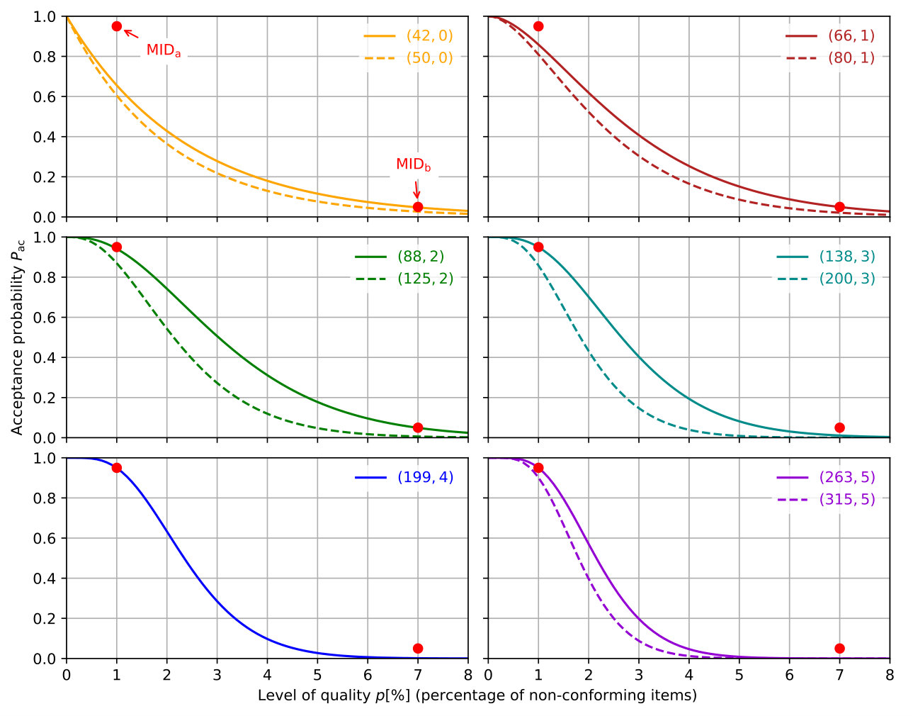 Figure 4
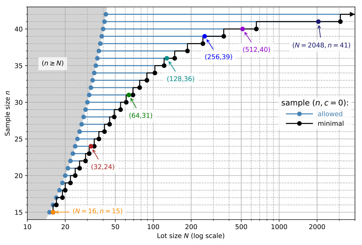 Figure 5
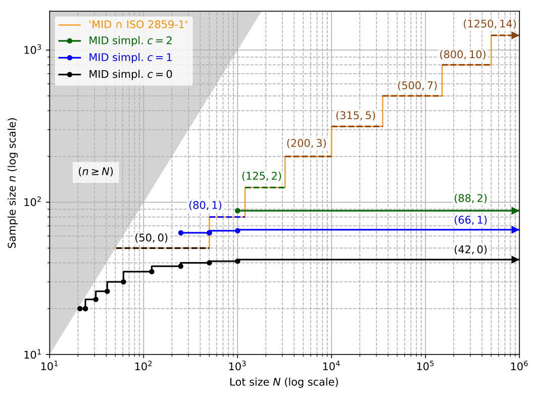 Figure 6
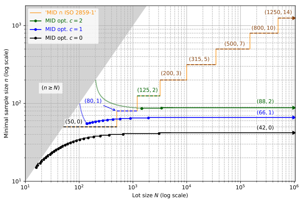 Figure 7
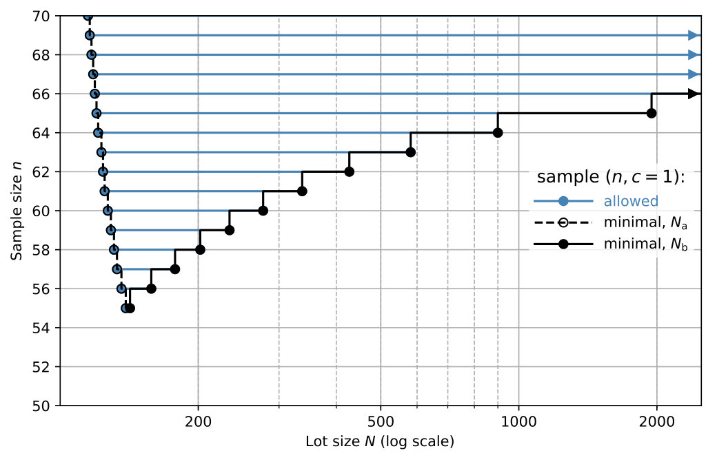 Figure 8
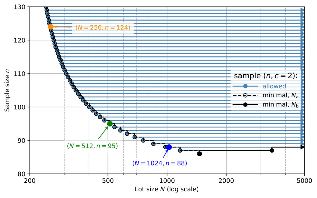 Figure 9
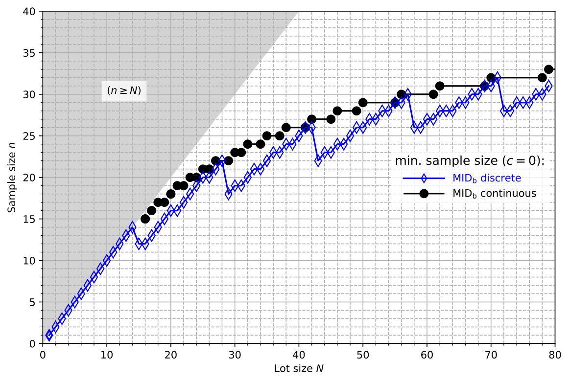 Figure 10
| % | % | % | % | % | ||
|---|---|---|---|---|---|---|
| 42 | 0 | 65.6 | 34.4 | 0.122 | 4.75 | 6.88 |
| 50 | 0 | 60.5 | 39.5 | 0.103 | 2.66 | 5.82 |
| 66 | 1 | 85.9 | 14.1 | 0.541 | 4.96 | 6.99 |
| 80 | 1 | 80.9 | 19.1 | 0.446 | 2.11 | 5.79 |
| 88 | 2 | 94.1 | 5.87 | 0.936 | 4.94 | 6.98 |
| 125 | 2 | 86.9 | 13.1 | 0.657 | 0.62 | 4.95 |
| 138 | 3 | 94.9 | 5.06 | 0.996 | 1.11 | 5.52 |
| 200 | 3 | 85.8 | 14.2 | 0.686 | 0.03 | 3.83 |
| 199 | 4 | 94.9 | 5.09 | 0.995 | 0.15 | 4.54 |
| - | 4 | - | - | - | - | - |
| 263 | 5 | 95.0 | 5.04 | 0.998 | 0.02 | 3.96 |
| 315 | 5 | 90.1 | 9.88 | 0.833 | 0.00 | 3.31 |
| Lot size | Sample | Producer’s risk [%] | Consumer’s risk [%] | ||||
|---|---|---|---|---|---|---|---|
| from | to | from | to | from | to | ||
| 15 | 16 | 15 | 0 | (40.37) | (32.21) | 0.00 | 4.15 |
| 17 | 17 | 16 | 0 | (34.53) | (34.53) | 3.00 | 3.00 |
| 18 | 19 | 17 | 0 | (36.82) | (32.66) | 2.13 | 4.46 |
| 20 | 20 | 18 | 0 | (34.73) | (34.73) | 3.42 | 3.42 |
| 21 | 22 | 19 | 0 | (36.77) | (33.94) | 2.61 | 4.05 |
| 23 | 24 | 20 | 0 | (35.84) | (33.74) | 3.19 | 4.31 |
| 56 | 61 | 30 | 0 | (34.76) | (33.70) | 4.36 | 4.94 |
| 62 | 69 | 31 | 0 | (34.81) | (33.66) | 4.36 | 4.99 |
| 70 | 78 | 32 | 0 | (34.71) | (33.71) | 4.43 | 4.99 |
| 79 | 89 | 33 | 0 | (34.72) | (33.77) | 4.45 | 4.98 |
| 90 | 103 | 34 | 0 | (34.73) | 33.81 | 4.47 | 4.97 |
| 104 | 122 | 35 | 0 | 34.74 | 33.83 | 4.48 | 4.98 |
| 123 | 148 | 36 | 0 | 34.71 | 33.85 | 4.51 | 4.99 |
| 149 | 187 | 37 | 0 | 34.70 | 33.86 | 4.54 | 5.00 |
| 188 | 248 | 38 | 0 | 34.66 | 33.89 | 4.57 | 5.00 |
| 249 | 363 | 39 | 0 | 34.66 | 33.91 | 4.59 | 5.00 |
| 364 | 659 | 40 | 0 | 34.65 | 33.93 | 4.61 | 5.00 |
| 660 | 3063 | 41 | 0 | 34.63 | 33.95 | 4.63 | 5.00 |
| 3064 | 42 | 0 | 34.62 | 34.4 | 4.65 | 4.75 | |
| Lot size | Sample | Producer’s risk [%] | Consumer’s risk [%] | ||||
|---|---|---|---|---|---|---|---|
| from | to | from | to | from | to | ||
| 139 | 142 | 55 | 1 | 5.07 | 5.26 | 4.88 | 4.98 |
| 136 | 158 | 56 | 1 | 5.05 | 6.37 | 4.33 | 4.98 |
| 133 | 178 | 57 | 1 | 5.02 | 7.41 | 3.83 | 4.99 |
| 131 | 202 | 58 | 1 | 5.04 | 8.35 | 3.39 | 4.99 |
| 129 | 234 | 59 | 1 | 5.05 | 9.26 | 2.98 | 4.99 |
| 127 | 277 | 60 | 1 | 5.04 | 10.10 | 2.61 | 5.00 |
| 125 | 337 | 61 | 1 | 5.00 | 10.88 | 2.27 | 5.00 |
| 124 | 427 | 62 | 1 | 5.08 | 11.62 | 1.99 | 5.00 |
| 123 | 581 | 63 | 1 | 5.14 | 12.31 | 1.74 | 5.00 |
| 121 | 900 | 64 | 1 | 5.05 | 12.97 | 1.48 | 5.00 |
| 120 | 1947 | 65 | 1 | 5.09 | 13.59 | 1.28 | 5.00 |
| 119 | 66 | 1 | 5.12 | 14.1 | 1.10 | 4.96 | |
| Lot size | Sample | Producer’s risk [%] | Consumer’s risk [%] | ||||
|---|---|---|---|---|---|---|---|
| from | to | from | to | from | to | ||
| 1454 | 1469 | 86 | 2 | 5.00 | 5.01 | 4.99 | 5.00 |
| 1166 | 3412 | 87 | 2 | 5.00 | 5.48 | 4.60 | 5.00 |
| 981 | 88 | 2 | 5.00 | 5.87 | 4.24 | 4.94 | |
| 852 | 89 | 2 | 5.00 | 6.03 | 3.90 | 4.68 | |
| 757 | 90 | 2 | 5.00 | 6.19 | 3.58 | 4.44 | |
| 684 | 91 | 2 | 5.00 | 6.36 | 3.28 | 4.21 | |
| 626 | 92 | 2 | 5.00 | 6.53 | 3.00 | 3.99 | |
| 579 | 93 | 2 | 5.00 | 6.70 | 2.74 | 3.78 | |
| 540 | 94 | 2 | 5.00 | 6.87 | 2.50 | 3.58 | |
| 508 | 95 | 2 | 5.00 | 7.04 | 2.28 | 3.39 | |
| 480 | 96 | 2 | 5.00 | 7.22 | 2.07 | 3.21 | |
| 257 | 123 | 2 | 5.03 | 12.62 | 0.08 | 0.70 | |
| 254 | 124 | 2 | 5.00 | 12.84 | 0.07 | 0.66 | |
| 252 | 125 | 2 | 5.02 | 13.07 | 0.06 | 0.62 | |
| Acceptance | Acceptance | Acceptance | ||||||||||
|---|---|---|---|---|---|---|---|---|---|---|---|---|
| Lot | Sample | Risk [%] | Sample | Risk [%] | Sample | Risk [%] | ||||||
| 21 | to | 24 | 20 | (43.4) | 0.69 | - | - | - | - | - | - | |
| 25 | to | 31 | 23 | (44.6) | 0.81 | - | - | - | - | - | - | |
| 32 | to | 41 | 26 | (40.6) | 1.90 | - | - | - | - | - | - | |
| 42 | to | 61 | 30 | (40.5) | 2.09 | - | - | - | - | - | - | |
| 62 | to | 122 | 35 | (40.1) | 2.30 | - | - | - | - | - | - | |
| 123 | to | 248 | 38 | 36.6 | 3.66 | - | - | - | - | - | - | |
| 249 | to | 500 | 40 | 35.4 | 4.21 | 63 | 12.2 | 3.77 | - | - | - | |
| 501 | to | 1000 | 41 | 34.9 | 4.48 | 65 | 13.4 | 4.23 | - | - | - | |
| 1001 | to | 42 | 35.0 | 4.44 | 66 | 14.1 | 4.45 | 88 | 5.87 | 4.25 | ||
Peer Reviews
No public reviews on file for this paper yet. If you reviewed it on a platform where reviews are public (OpenReview, ICLR, NeurIPS, ICML), you can paste yours below so the community can read it here.
Videos
No videos yet. Explain this paper in a talk, walkthrough, or lecture? Add one.
Optimal acceptance sampling for modules F and F1 of the European Measuring Instruments Directive
Cord A. Müller
German Academy of Metrology (DAM),
Bavarian State Office for Weights and Measures (LMG),
Wittelsbacherstr. 17, 83435 Bad Reichenhall, Germany [email protected]
Abstract
Acceptance sampling plans offered by ISO 2859-1 are far from optimal under the conditions for statistical verification in modules F and F1 as prescribed by Annex II of the Measuring Instruments Directive (MID) 2014/32/EU, resulting in sample sizes that are larger than necessary. An optimised single-sampling scheme is derived, both for large lots using the binomial distribution and for finite-sized lots using the exact hypergeometric distribution, resulting in smaller sample sizes that are economically more efficient while offering the full statistical protection required by the MID.
Contents
1 Introduction
The European Measuring Instruments Directive 2014/32/EU (MID) [1] states in Annex II that the statistical verification of products in modules F and F1 must respect the following conditions:
“The statistical control will be based on attributes. The sampling system shall ensure:
- (a)
a level of quality corresponding to a probability of acceptance of 95%, with a non-conformity of less than 1%;
- (b)
a limit quality corresponding to a probability of acceptance of 5%, with a non-conformity of less than 7%.”
These wordings must be cast into mathematical equations in order to determine acceptance sampling plans to be used in practice, as described by the pioneering work of Dodge and Romig [2]. There appears to be consensus among the legal bodies in charge of administering the tests [3] that the MID conditions should be interpreted as
[TABLE]
Here is the quality level or “fraction defective”, namely the fraction of non-conforming111We use the terms “non-conforming” and “defective” interchangeably for items that fail testing. items in the lot, and is the acceptance probability, a property of the statistical sampling plan to be devised. The first quality level is commonly called the acceptance quality limit (AQL). The complement of the acceptance probability at this point, , is known as the producer’s risk that a lot with this acceptable level of quality is rejected. The second quality level is known as the limiting quality (LQ), and the probability of acceptance is the consumer’s risk of accepting a lot with this doubtful quality.
Since a lower quality level (i.e., larger ) should result in a lower acceptance probability, a valid function is strictly decreasing: .222For finite lot sizes, may not be strictly monotonic, but just monotonic. The MID conditions (1) and (2), however, implicitly assume an infinite lot size; for details see Appendix A below. Therefore, the two conditions (1) and (2) for a certain sampling plan to be valid can be formulated equivalently
[TABLE]
In other words, the MID conditions in the prevailing interpretation require
- (a)
a lot with AQL to imply a producer’s risk
[TABLE] 2. (b)
and a lot with LQ to imply a consumer’s risk
[TABLE]
As a consequence, the graph of , the so-called operating characteristic (OC), must lie below and left of the two points \text{MID{}{\text{a}}{}}=(p_{\text{a}},P_{\text{a}}) and \text{MID{}{\text{b}}{}}=(p_{\text{b}},P_{\text{b}}). Figure 1 shows, as an example, 3 OCs of different single-sampling plans for very large lots, based on the binomial model of Section 2. Too small samples are typically ruled out because their OCs violate the MID conditions by lying above at least one MID point, as illustrated by the plan with sample size and acceptance number . In contrast, large samples and large acceptance numbers will typically result in OCs that are far below the MID points; thus they are certainly admissible. As an example, Fig. 1 shows the OC of , , a member of the ISO 2859-1 family [4] that is recommended officially [3] for lot sizes from 150 001 till 500 000. However, such a sampling is clearly biased toward a much better quality level than required by the MID conditions.
Sampling plans favouring very low AQLs are deemed admissible because the prevailing interpretation of the MID conditions implies a producer’s risk larger than 5% [Eq. (5)]. The main point of the present work is that a sampling plan that is fair and economically acceptable for producers should not impose arbitrary conditions on the producers much stricter than required by the MID, while respecting the legitimate interests of the consumers, of course. Therefore, MID-optimised sampling plans outside the scope of ISO 2859-1 are derived in the following sections, devoted to very large lots (Sec. 2) and finite-sized lots (Sec. 3), respectively. Readers not interested in details of the mathematical derivation are invited to skip to Sec. 4, where a simplified single-sampling scheme optimised for MID modules F and F1 is proposed.
The concluding Sec. 5 finishes on the observation that it would seem more reasonable if the sampling contract between producer and consumer bounded both their risks from above, guaranteeing both and . This alternative interpretation of the MID’s AQL condition has interesting consequences that are briefly outlined, with details relegated to a follow-up paper.
2 MID-optimised sampling plans for large lots
In a first step, let us consider single sampling where items are drawn from a very large lot with a constant (but generally unknown) probability to be defective.333Strictly, a probability for a draw without replacement can only stay constant when the lot size is infinite; for now we assume and consider corrections due to finite lot size in Sec. 3 below. The entire lot is accepted if the number of defective items discovered by testing is not larger than the acceptance number . The acceptance probability to find at most defective items, each found independently from the others with identical probability , in a sample of size is the cumulative binomial distribution [5, 6]
[TABLE]
where the binomial coefficient counts the number of different choices of items among .
Figure 2 shows the resulting OCs for various single-sampling plans , grouped with increasing acceptance number into pairs. The dashed curve shows the respective member of the ISO 2859-1 family at inspection level II as recommended in [3].444For , ISO 2859-1 offers no sample size. Instead, it jumps directly from to . The full curve shows the smallest sample compatible with both MID conditions, which can be computed using standard numerical tools or commercial software, lowering the sample size until one of the two MID conditions is violated. Not surprisingly, when relaxing the constraint to the somewhat arbitrary members of the ISO 2859-1 family, one obtains considerably smaller sample sizes. Qualitatively, one arrives at the same conclusion when approximating the binomial distribution (7) for , at fixed by the cumulative Poisson distribution . Indeed, the respective minimal sample sizes under the Poisson approximation are, for , , for , , for , , for , , for , , for , , etc. Here, each number in parentheses denotes the difference to the optimal, and more accurate binomial result displayed in the first two columns and grey-colored rows of Table 1.
Because the probabilities for the different cases in Eq. (7) add up and still must stay below the MID points, the minimum sample size grows with the acceptance number. In return, the OCs gain in specificity (smaller ) and sensitivity or statistical power (smaller ), i.e., permit to distinguish more accurately between high and low quality levels. For small acceptance numbers , the LQ condition of MID is the more stringent, i.e., OCs are not steep enough. For large acceptance numbers , the AQL condition of MID becomes more stringent, i.e., OCs are steeper than required. The optimal sample plan, with smallest sample size while least biased with respect to both MID conditions, is found to be .
Table 1 lists the corresponding data, allowing for a quantitative comparison of the ISO 2859-1 and MID-optimised sample plans. As Fig. 2 already shows, the LQ criterion MID can be saturated quite well for low acceptance numbers, with a consumer’s risk quality (CRQ) such that not much below , and a consumer’s risk not much below . The price to be paid for small acceptance numbers and sample sizes is an elevated producer’s risk , i.e., a high probability for the type I error of rejecting a good lot. And the smallest admissible member of the ISO 2859-1 family at inspection level II is stricter than necessary with a producer’s risk of ; the corresponding producer’s risk quality (PRQ) required to reach is as low as . The minimal single-sampling plan compatible with MID conditions implies a slightly smaller producer’s risk with a slightly larger PRQ of and a CRQ just below .
Conversely, for larger acceptance numbers and, thus, larger sample sizes, the AQL criterion MID becomes saturated with a producer’s risk approaching from above. Here, the consumer’s risk drops to values much lower than required by MID, and a CRQ substantially smaller than . Larger samples are indeed generally known to reduce the probabilities of type I and II errors and to have a greater discriminating power [5, 6]. Thus, larger samples and higher acceptance numbers have their merits in internal production control and may well be suggested in the corresponding MID modules. However, a systematic growth of sample size with lot size, as recommended by the ISO 2859-1 sampling system, is not warranted by the MID conditions for modules F and F1.
In summary so far: For large enough lot sizes (see Section 3.4 for a quantitative discussion) the minimal, least biased sample plan for statistical product verification in the MID modules F and F1 is .
3 Finite lot sizes
If the lot size is not much larger than the sample size then finite-size corrections become noticeable, and the results of the previous section have to be revisited [5]. Let us consider a sample of items drawn without replacement from a lot of size containing defective items. Under the single-sampling paradigm, the lot is to be accepted if the sample contains at most defective items. The acceptance probability is then given by the cumulative density of the hypergeometric distribution,
[TABLE]
where each summand is the combinatorial probability to find exactly defective items among the items tested. One can assign the quality level to this lot and discuss its acceptance probability for fixed as function of the operationally meaningful values , where
[TABLE]
is the domain of the function .
From this general setting follows
Proposition 1**.**
A single-sampling plan with acceptance number can only be admissible under the MID condition (3) for lot sizes
[TABLE]
Proof.
A lot containing at most defective items will certainly be accepted by any sample plan . But then the corresponding quality level (where ) must be smaller than the AQL since otherwise condition (3) cannot be satisfied. Therefore, , which is equivalent to (10). ∎
Analogously to the optimisation of sample size in Section 2, one can further determine the smallest sample size , given acceptance number and lot size , that is admissible under the MID conditions. We choose to use the criteria (3) and (4), namely checking whether the acceptance probability (8) at and is inferior to the bounds and , respectively. This requires the extension of the factorials in (8) to non-integer arguments, which is easily achieved using the gamma function [7]:
[TABLE]
While the notion of non-integer values for and is not evident to justify operationally for single lots, this procedure turns out to be more consistent than a purely discrete formulation; for a detailed justification see Appendix A.
We find that the manner in which finite lot size affects MID-optimised sample plans depends crucially on the acceptance number. Details for the most relevant cases are discussed in the following subsections 3.1 through 3.3. Readers mainly interested in the final results are invited to consult Sec. 3.4 straight away.
3.1 Zero acceptance
For , the binomial prediction for very large lots () is conservative in the sense that it overestimates the sample size that is really necessary for a lot of a certain finite size [5]. Thus, from ISO 2859-1 has been correctly identified as being compatible with MID for lot sizes from [3]. Similarly, the single-sampling plan is certainly admissible, all the way down to . However, taking into account finite lot sizes allows us to reduce the required sample sizes even further.
Let us first explain qualitatively why smaller lots require smaller zero-accceptance samples. In the binomial model, the probability to draw defective items without replacement from the lot is taken constant. However, if a lot of size contains defective items, then the fraction defective is only for the first draw. The probabilities of the second draw depend on the outcome of the first. If the first item is defective, then the second item is defective with probability , which is smaller than (we can assume , since for one has , a trivial case without practical interest because all lots are rejected anyway). Vice versa, if the first item is conforming, then , which is larger than (we assume , otherwise we have , again a trivial case where all lots are accepted). The latter case is more frequent since in realistic settings. This evolution of the probability to larger values will likely continue for each draw, so that the actual chance to discover defective items in a lot of small size is larger than predicted by the binomial model. By consequence, the actual acceptance probability for the same sample size would be smaller, such that a smaller sample actually suffices to stay below the MID bounds.
For , the general expression (8) for the acceptance probability simplifies somewhat,
[TABLE]
With the help of the factorial extension (11), one can determine numerically the smallest sample size , given the lot size , that still fulfills both MID conditions. It turns out that actually only the LQ condition (4) at MID matters. Figure 3 shows the result of such a minimisation, for lot sizes growing in geometric progression toward the limit where the binomial result of Section 2 becomes exact. It is evident that sample sizes can be substantially reduced compared to the binomial model for small to moderate lot sizes.
In theory, the smallest lot size for which statistical sampling can be envisaged under the MID conditions is . The reason is that for , the quality level of a lot with a single defective item is at least and thus already larger than that should be rejected. Therefore, the only way to ensure MID conditions for is 100% testing with . The next larger lot size is such that a sample size of violates condition (4). Thus, also requires 100% testing with . The combination and , however, is compatible with the MID conditions, as shown by the corresponding OC in Fig. 3. For , one has to step up to , and so on, all the way up to and . From onward, the required sample size saturates at already derived from the binomial model (cf. Fig. 2). Figure 4 shows the allowed and minimum sample size found under MID conditions as function of the lot size .
The corresponding lot-size intervals with their minimum sample sizes are listed in Table 2, together with the producer’s and consumer’s risks. Since the sample size is optimised with respect to the MID conditions (here, for , only the consumer’s point MID matters), these data vary only slightly from one case to the other. The main message is that sample size can be substantially reduced, under very similar risks, for finite lot sizes all the way down to .
3.2 Unit acceptance
Just as for , one can minimize the sample size for a given with fixed such that the MID conditions are fulfilled. In contrast to the case , now also the producer’s point MID plays a significant role, which brings about a qualitative difference in the behavior of the OCs as function of system size . Indeed, Eq. (10) of Proposition 1 tells us already that the lot size is globally bounded from below by . The precise value of this lower bound depends on the acceptance probability at the AQL point MID and thus on the sample size . Conversely, the lot size is bounded from above, at fixed sample size, by the behaviour at the LQ point MID. Figure 5 shows the resulting, allowed combinations of sample size and lot sizes . No MID-compatible sampling with is possible. As shown by the ‘a’ branch on the left side, the MID point requires the minimum sample size to grow sharply when the sample size decreases toward the absolute lower bound (10) at . For all larger lot sizes , the sampling already known from the binomial model becomes optimal.
Table 3 shows the quantitative risk data associated with these intervals. By construction, for the smallest allowed lot size in each row (the “from” case), the producer’s risk is optimally close to (and just above) the limit 5% imposed by the AQL point MID; conversely, for the largest allowed lot size (the “to” case), the consumer’s risk is optimally close to (and just below) the 5% limit imposed by the LQ point MID.
3.3 Double acceptance
For , now the AQL point MID mainly determines the allowed combinations of lot size and sample size . For an illustration, Figure 6 shows the OCs of 3 different sample sizes with their minimum sample sizes determined by the MID condition. Since the binomial limit is conservative in the sense that the acceptance probability (8) at increases as lot size decreases, then the minimum sample size has to increase as well for smaller lots in order to compensate this effect. This one-sided constraint makes the MID point increasingly irrelevant as becomes smaller, as evident from the OC for the smallest lot size plotted in Fig. 6. The rapid decrease of the OC indicates that the acceptance number is too elevated for such a small lot size, suggesting instead to fall back onto or even .
Figure 7 shows the allowed combinations of lot and sample sizes. The minimum sample size found from the binomial model, , is admissble only down to . For smaller lots, the minimum sample size has to increase quite dramatically in order to satisfy the MID condition. The MID constraint only has a marginal influence: it limits the validity of the smallest possible sample sizes to , respectively. The optimal binomial result is valid up to arbitrarily large lots, of course.
Table 4 lists the allowed sample size as function of the lot size intervals, together with the producer’s and consumer’s risks. It is clear that for smaller lots, double-acceptance sampling is no longer the best choice for a fair realization of the MID criteria. For example, a lot of size requires the minimum double-acceptance sampling and features only a consumer’s risk of , two orders of magnitude smaller than required by MID. An arguably better choice then is , for which it can be found in Table 3 that the smallest allowed unit-acceptance sampling has and .
3.4 Summary of results for finite lot sizes
Figure 8 summarizes the impact of finite lot sizes on the MID-optimised sampling scheme with acceptance number , covering several orders of magnitude on a double logarithmic scale. The main results are:
The minimal sample plans obtained within the binomial model for large lots in Sec. 2, , , and , are indeed the minimal sample plans for all lot sizes where , , and . Finite-lot-size corrections are of two different types, dictated by the two different MID conditions. Their respective effects appear depending on the acceptance number: 2. 2.
Acceptance number : The minimal binomial sampling plan is conservative in the sense that it remains formally admissible down to . But for lot sizes smaller than , smaller samples are possible because it becomes easier to satisfy the only relevant condition (4) at LQ . The minimum sample size as function of lot size is listed in Table 2 and shown in Figs. 4 and 8. 3. 3.
Acceptance number : The minimal binomial result is no longer globally conservative. Certainly, below , the necessary sample size first decreases for smaller lots because it becomes easier to satisfy the LQ condition (4). But below a lot size of , where the smallest possible sample size is , now the AQL condition MID takes over. It requires the sample size to grow quite sharply with decreasing lot size in order to ensure an acceptance probability at below . This sharp upturn continues down to , where the global lower bound (10) is reached. The admissible (minimum) sample size as function of lot size is listed in Table 3 and plotted in Fig. 5 (Fig. 8). 4. 4.
Acceptance number : The minimal binomial result is not globally conservative. Mainly the AQL condition (3) at MID is relevant, requiring the minimum sample size to grow for decreasing lot size. This sharp upturn continues down to , where the global lower bound (10) is reached. The admissible (minimum) sample size as function of lot size is listed in Table 4 and plotted in Fig. 7 (Fig. 8). Below roughly , the consumer’s risk drops far below the MID threshold such that acceptance sampling becomes more appropriate. 5. 5.
Figure 8 also shows the ISO 2859-1 sampling plans recommended officially for MID modules F and F1 [3]. Clearly, these are not minimal for low acceptance numbers . Moreover, their growth with sample size, roughly as , is not justified by the MID conditions as read in Sec. 1. By contrast, the MID-optimised sample plans derived here for remain valid for arbitrarily large lots.
4 Simplified single-sampling scheme
The numerical minimisation of sample size as function of lot size under MID conditions produces the sample plans that are listed in Tabs. 2, 3 and 4 for , respectively. Admittedly, these tables (and corresponding figures) are more complicated than the sample plans extracted from ISO 2859-1 that are recommended hitherto [3]. It appears therefore advisable to condense the optimised plans into a simplified sampling system that is still (almost) optimal as far as the MID conditions are concerned, but efficient to use in practice. Table 5 contains a proposal for such a sampling system, retaining the essential characteristics of the MID-minimised sampling plans. Figure 9 represents this simplified scheme, to be compared to the exact data represented in Fig. 8. The main steps taken to arrive at the simplified scheme are:
- •
choosing a simple lower bound common to the relevant, minimal binomial sampling plans , , and ;
- •
binning lot sizes into a manageable number of intervals common to all relevant acceptance numbers .
Such a simplified proposal is slightly arbitrary in the sense that one may as well choose different lot-size intervals with, consequently, a different set of sample sizes. The present proposal aims at a reasonable compromise between the complexity of the scheme and its logistic efficiency. Independently of the finer details, the main feature of our proposal is that the sample size does not grow with the lot size above , while offering the full statistical protection required by the MID.
For small lot sizes , only zero-acceptance sampling is found to be practical, with advantageously small samples but rather elevated producer’s risks. The larger the lot, the more options are offered for statistical sampling. So one thing remains to be specified: Which acceptance number should be chosen above , and which of above ? Only if the producer knows in advance that the quality level of the lot is perfect ( by production or strict exit controls), then with the smallest possible sample size is of course preferable. If the quality level is finite () but unkown, then the choice of the sample plan is not uniquely determined by the MID conditions. Instead, the producer may decide which risk is worth taking, depending on the lot’s known or expected quality level, the production cost of each item, its inspection cost, etc.. If, on the one hand, production costs are low, but inspection costs are high, then an elevated producer’s risk may be acceptable, and the smallest acceptance number is preferable with, consequently, the smallest sample size. If, on the other hand, production costs are high and inspection costs are low, then the producer’s risk can be substantially reduced by raising the acceptance number to , together with an altogether moderate increase of sample size. In order to arrive at a truly (or at least approximately) optimal choice, one would have to define an appropriate cost function and determine the optimal acceptance number by an in-depth cost-benefit analysis [8].
5 Outlook: alternative interpretation of the AQL criterion
The AQL criterion of the MID, interpreted as in expressions (1),(3), and (5), sets a lower bound on the producer’s risk. This is a somewhat curious condition, already from an economic and contractual point of view: why should the MID guarantee a one-sided protection of the consumer’s interest at two points, without limiting the producer’s risk at the acceptance quality level? Furthermore, this condition leads to a number of awkward mathematical properties that belie standard statistical knowledge in acceptance sampling. For example, the binomial approximation for the true hypergeometric distribution is known to be conservative in the sense that it provides larger samples than necessary for a certain finite lot size [5]. This turns out not to be true here for sampling in the lot-size range where the AQL condition dominates and requires larger samples than the binomial approximation.
Indeed, standard textbooks formulate the AQL inequality usually the other way around, setting an upper bound also on the producer’s risk—see, e.g., Eq. (10.57) in [6]. Additionally, an upper bound on both the consumer’s and producer’s risk is compatible with the framework of hypothesis testing (see, e.g., section 2.2 in [9]), which could have important conceptual and operational benefits [10]. Details of MID-optimised sampling plans obtained under such an alternative interpretation of the MID’s AQL criterion, however, are beyond the scope of the present work and will be presented in a forthcoming publication.
Acknowledgements
The author is indebted to Dr. Katy Klauenberg for a critical reading of the manuscript and insightful comments.
Appendix A Interpretation of MID criteria for finite lots
We need to discuss the applicability of the MID criteria, either (1) and (2) or (3) and (4), for isolated lots of finite size, where quality levels and acceptance probabilities are discrete sets. Consider a lot of size , containing an (unknown) number of non-conforming items. One can assign the quality level to this lot and discuss its acceptance probability under a certain sampling plan as function of the meaningful values
[TABLE]
Now, the two special quality levels of the MID conditions, and , are only in the domain if is an integer multiple of 100. For all other lot sizes, such that as given by eq. (8) is not defined, at least not in simple operational terms related to the sampling of a single lot, where must be an integer. As a consequence, the MID conditions (3) and (4) cannot be applied as such for deciding whether a sampling plan is admissible or not. And even if per chance is a multiple of 100, also the image of under , the set of the different acceptance probabilities, is now a discrete set that will generally not contain the two values and . In other words, in most cases there will be no such that , exactly. Thus, also the MID conditions (1) and (2) cannot be applied as such.
It thus becomes clear that the wording of the MID implicitly assumes a continuous description, which applies only to process sampling with a formally infinite lot size (called “type B” in [5, 6]). However, the MID product testing in modules F and F1 typically involves isolated lots of finite size, where the continuity of type B testing cannot be taken for granted. In a first attempt to render the MID conditions meaningful for finite lot sizes, we have tried to interpret the wording “corresponding to a probability of acceptance of ” as meaning “corresponding to a probability of acceptance of at least ”.555In the continuous case, this follows already from the monotonicity and continuity of : There is exactly one such that and for which MID implies . Now take any such that . The monotonicity () in its negated form then implies together with the r.h.s. . So the MID conditions could have been formulated with a “probability of at least ” from the start. Then, the two MID conditions (1) and (2) are rather
[TABLE]
which can be tested for all . A logically equivalent, but more practical criterion that can be readily evaluated with a computer is obtained by the negation of (14), namely
[TABLE]
Under these premises, in order to test the admissibility of a certain sampling plan, one only needs to take the first allowed quality levels larger than or equal to and , respectively, and check whether at these points is smaller than and , respectively. If that is the case, then the plan is approved (monotonicity guarantees that even larger cannot yield larger values of ), and if not, it is rejected.
While this interpretation is logically satisfying and economical to evaluate, it leads to inconsistencies due to discretisation effects. Indeed, when the lot size is increased such that one quality level drops below , the next higher quality level becomes relevant such that suddenly a smaller sample may become allowed. Figure 10 shows the minimum sample size as function of lot size resulting from the purely ‘discrete’ criterion (15). It features a prominent saw-tooth structure where raising the lot size at certain points (e.g., from to 43) suddenly lowers the minimum sample size (e.g., from to 22).
Such an erratic dependence of sample size on lot size is arguably not a desirable feature of an acceptance sampling plan. Therefore, we have proposed in Sec. 3.1 to extend the acceptance probabilities in the standard manner to non-integer item numbers, formally adopting a type-B testing scenario that allows us to evaluate at and for any lot size and thus to use the MID criteria (3) and (4) just as in a truly continuous case. The advantage is two-fold: First, the resulting sample size is conservative, namely, never smaller than prescribed by the discrete criterion (15) at the consumer’s LQ point, where also the binomial model for infinite lots is conservative. Second, the minimum lot size resulting from the consumer’s LQ point condition is a non-decreasing function of lot size, as evident from Fig. 10 (see also Fig. 4 and the relevant portion of Fig. 5).
The reference list from the paper itself. Each links out to its DOI / PubMed record.
- 1[1] Directive 2014/32/EU of the European Parliament and of the Council of 26 February 2014 on the harmonisation of the laws of the Member States relating to the making available on the market of measuring instruments (recast), OJ L 96/149 (2014)
- 2[2] H F. Dodge, H. G. Romig, ”A Method of Sampling Inspection”, Bell Syst. Tech. J. 8 , 613-631, 1929 · doi ↗
- 3[3] WELMEC European cooperation in legal metrology: Working group 8, Measuring Instruments Directive (2014/32/EU): Guide for generating sampling plans for statistical verification according to Annex F and F 1 of MID 2014/32/EU (2018)
- 4[4] ISO/TC 69/SC 5, ”Sampling procedures for inspection by attributes - Part 1: Sampling schemes indexed by acceptance quality limit (AQL) for lot-by-lot inspection”, ISO 2859-1:1999(E)
- 5[5] E.G. Schilling, D. V. Neubauer, Acceptance Sampling in Quality Control (CRC Press, Boca Raton, 2017)
- 6[6] P. Mathews, Sample Size Calculations. Practical Methods for Engineers and Scientists (Mathews Malnar and Bailey, Fairport Harbor, 2010).
- 7[7] M. Abramowitz and I. A. Stegun (eds.), The Handbook of Mathematical Functions with Formulas, Graphs, and Mathematical Tables National Bureau of Standards Applied Mathematics Series 55 (1972).
- 8[8] H. F. Campbell and R. Brown, “Incorporating Risk in Benefit-Cost Analysis”. Benefit-Cost Analysis: Financial and Economic Appraisal using Spreadsheets (Cambridge University Press, Cambridge, 2003)