Thermonuclear fusion rates for tritium + deuterium using Bayesian methods
Rafael S. de Souza, S. Reece Boston, Alain Coc, Christian Iliadis
TL;DR
This paper employs Bayesian methods to accurately determine thermonuclear fusion rates for the tritium-deuterium reaction, incorporating comprehensive parameter uncertainties and challenging previous claims of electron screening effects.
Contribution
It introduces a Bayesian R-matrix model that includes all relevant parameters and uncertainties, providing more reliable fusion rate estimates for astrophysics and fusion energy applications.
Findings
Reaction rate uncertainties are between 0.2% and 0.6%.
Reaction rates differ by up to 2.9% from previous results.
No evidence of electron screening effects was found.
Abstract
The H(d,n)He reaction has a large low-energy cross section and will likely be utilized in future commercial fusion reactors. This reaction also takes place during big bang nucleosynthesis. Studies of both scenarios require accurate and precise fusion rates. To this end, we implement a one-level, two-channel R-matrix approximation into a Bayesian model. Our main goals are to predict reliable astrophysical S-factors and to estimate R-matrix parameters using the Bayesian approach. All relevant parameters are sampled in our study, including the channel radii, boundary condition parameters, and data set normalization factors. In addition, we take uncertainties in both measured bombarding energies and S-factors rigorously into account. Thermonuclear rates and reactivities of the H(d,n)He reaction are derived by numerically integrating the Bayesian S-factor samples. The present…
Click any figure to enlarge with its caption.
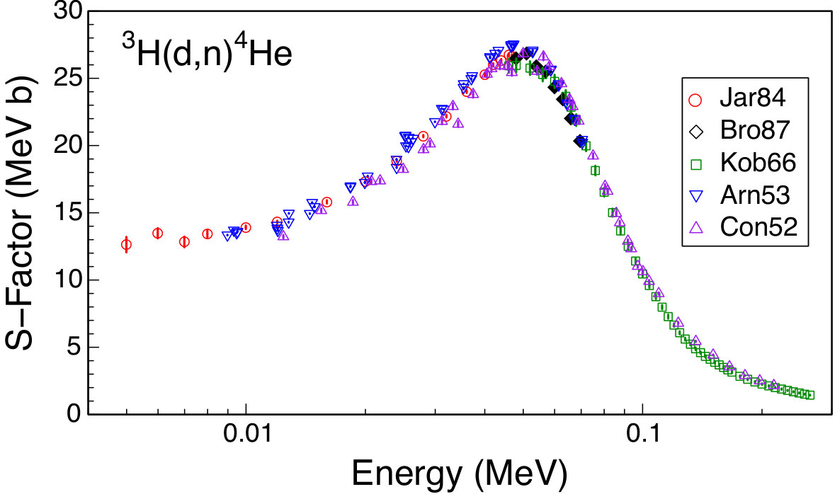 Figure 1
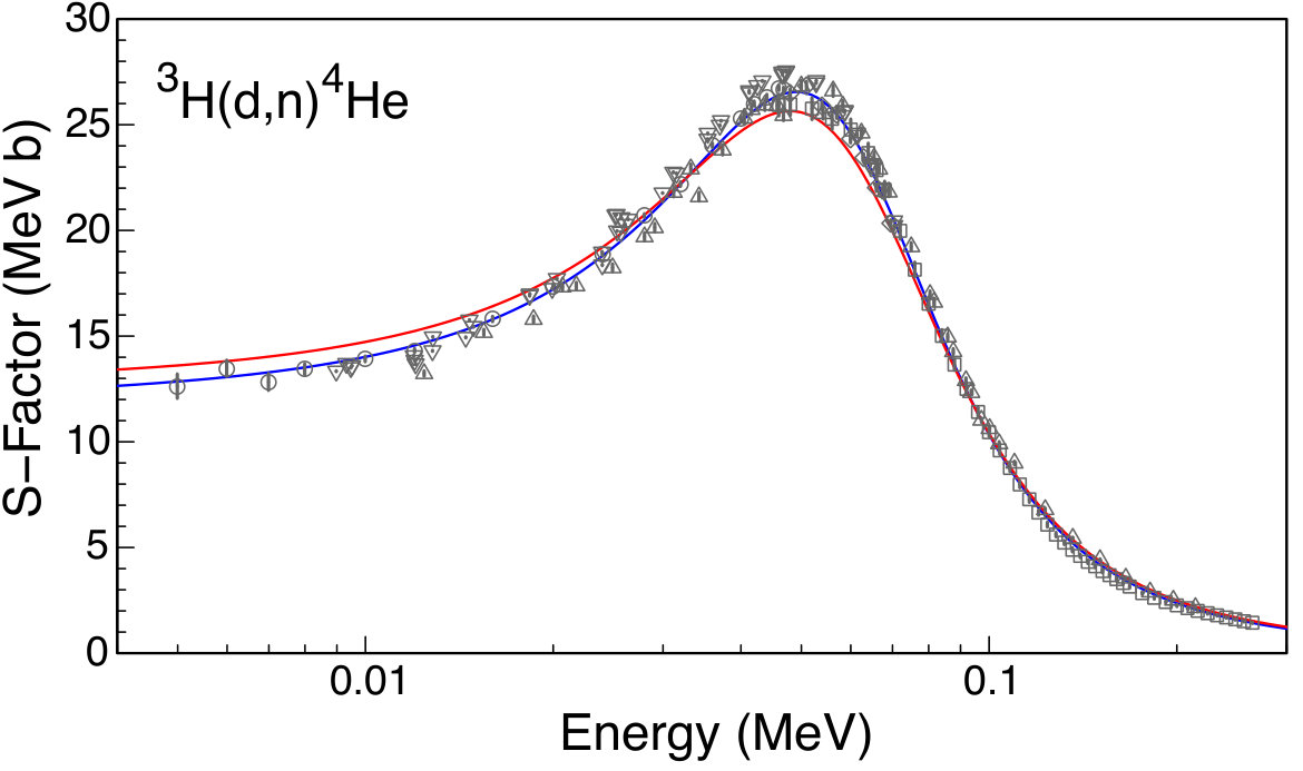 Figure 2
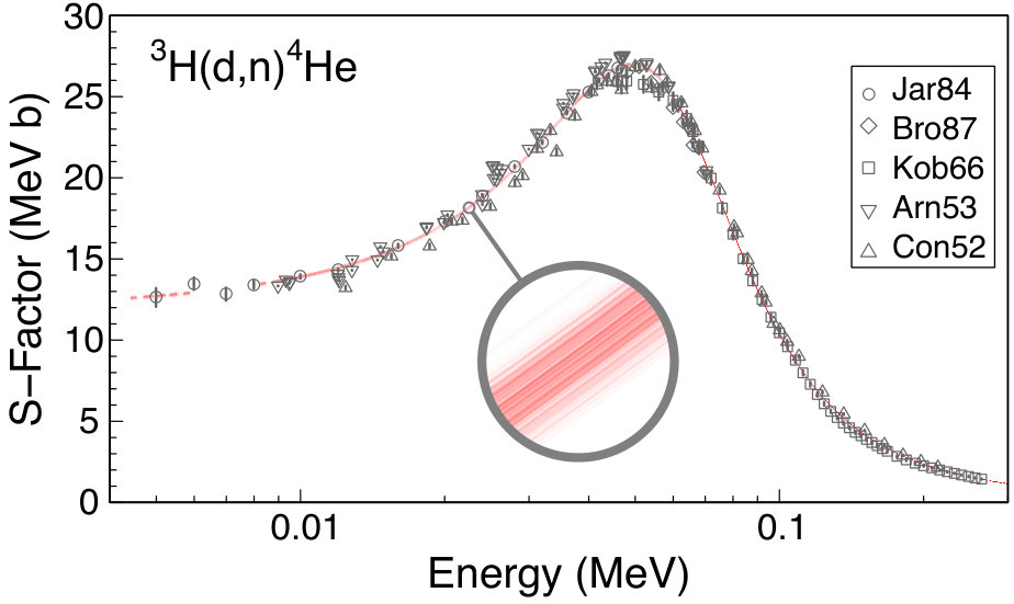 Figure 3
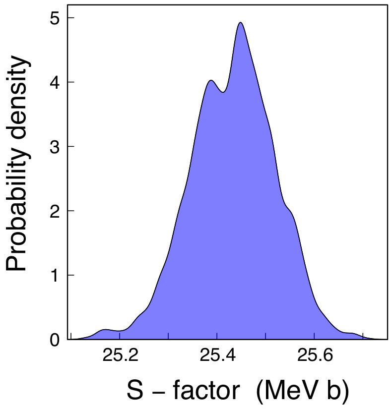 Figure 4
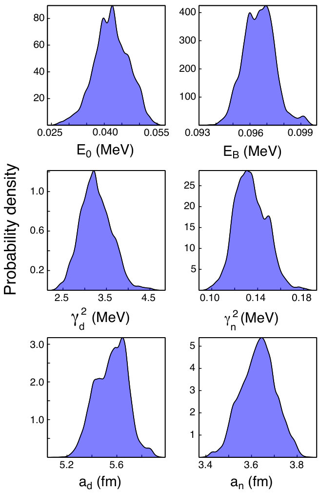 Figure 5
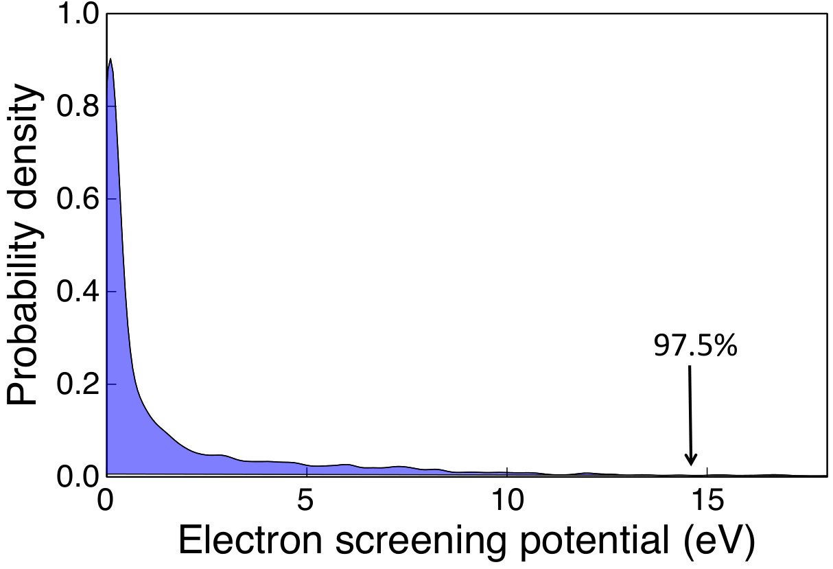 Figure 6
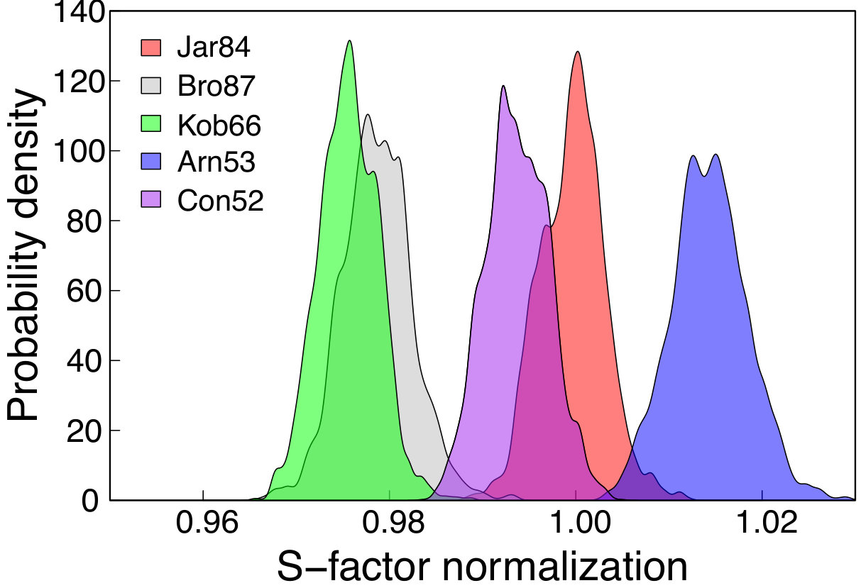 Figure 7
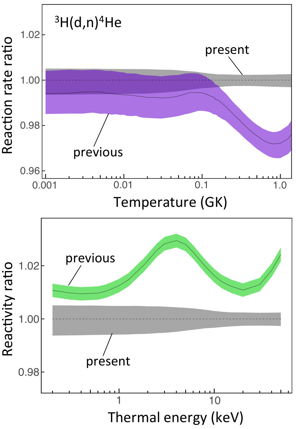 Figure 8
| Parameter | Present111Uncertainties represent th, th, and th percentiles, while upper limits correspond to % credibility. | Previous |
|---|---|---|
| (MeV) | 0.0420 | 0.0912222From Ref. Barker (1997); his fit was performed with the condition and with fixed channel radii ( fm, fm). No uncertainty estimates were provided. |
| (MeV) | 0.09654 | 0.0912222From Ref. Barker (1997); his fit was performed with the condition and with fixed channel radii ( fm, fm). No uncertainty estimates were provided. |
| (MeV) | 3.23 | 2.93666From Ref. Barker (1997); no uncertainty estimates were provided. |
| (MeV) | 0.133 | 0.0794666From Ref. Barker (1997); no uncertainty estimates were provided. |
| (fm) | 5.56 | 7.0333From Refs. Argo et al. (1952); Hale et al. (2014). No uncertainty estimates were provided, and both works assumed . |
| (fm) | 3.633 | 7.0333From Refs. Argo et al. (1952); Hale et al. (2014). No uncertainty estimates were provided, and both works assumed ., 5.51.0444From Ref. Woods et al. (1988), who assumed ., 2.9555From Refs. Adair (1952); Dodder and Gammel (1952); no uncertainty estimates were provided. |
| (MeV) | 0.897777Calculated from the sampled reduced width values, and , at the sampled energy values, . | |
| (MeV) | 0.549777Calculated from the sampled reduced width values, and , at the sampled energy values, . | |
| (eV) | or 888From Ref. Langanke and Rolfs (1989); the first and second value is obtained from the Thomas-Fermi model and the Hartree-Fock model, respectively. | |
| (MeVb)999S-factor at keV. | 25.438 | 25.870.49101010From Table V of Ref. Bosch and Hale (1993a); the uncertainty of 1.9% provided in their Table IV has no rigorous statistical meaning, but signifies the “maximum deviation of the approximations from the original R-matrix cross-sections.” |
| Parameter111The symbols , , , and denote the extrinsic uncertainty in energy and S-factor, the systematic energy shift, and the S-factor normalization, respectively; the indices, , label the five different data sets: (1) Jarmie, Brown and Hardekopf Jarmie et al. (1984a); (2) Brown, Jarmie and Hale Brown et al. (1987); (3) Kobzev, Salatskij and Telezhnikov Kobzev et al. (1966); (4) Arnold et al. Arnold et al. (1953); (5) Conner, Bonner and Smith Conner et al. (1952). | Value222Uncertainties represent th, th, and th percentiles, while upper limits correspond to % credibility. |
|---|---|
| (eV) | 0.23 |
| (eV) | 0.5 |
| (eV) | 81 |
| (eV) | 3.5 |
| (eV) | 6 |
| (eV) | 1.1 |
| (eV) | 3.0 |
| (eV) | 153 |
| (eV) | 2.9 |
| (eV) | 11 |
| 0.9998333Ref. Brown and Hale (2014) report normalization factors of and for the data of Ref. Jarmie et al. (1984a) and Ref. Brown et al. (1987), respectively, where their value corresponds to the inverse of our value of (see Section IV.3). | |
| 0.9786333Ref. Brown and Hale (2014) report normalization factors of and for the data of Ref. Jarmie et al. (1984a) and Ref. Brown et al. (1987), respectively, where their value corresponds to the inverse of our value of (see Section IV.3). | |
| 0.9756 | |
| 1.0143 | |
| 0.9936 | |
| (MeVb) | 0.112 |
| (MeVb) | 0.181 |
| (MeVb) | 0.0285 |
| (MeVb) | 0.471 |
| (MeVb) | 0.559 |
| T (GK) | Median111Reaction rates in units of cm3 mol-1 s-1, corresponding to the 50th percentile of the rate probability density function. The rate factor uncertainty, , is obtained from the 16th and 84th percentiles (see the text). | 111Reaction rates in units of cm3 mol-1 s-1, corresponding to the 50th percentile of the rate probability density function. The rate factor uncertainty, , is obtained from the 16th and 84th percentiles (see the text). | T (GK) | Median111Reaction rates in units of cm3 mol-1 s-1, corresponding to the 50th percentile of the rate probability density function. The rate factor uncertainty, , is obtained from the 16th and 84th percentiles (see the text). | 111Reaction rates in units of cm3 mol-1 s-1, corresponding to the 50th percentile of the rate probability density function. The rate factor uncertainty, , is obtained from the 16th and 84th percentiles (see the text). |
|---|---|---|---|---|---|
| 0.001 | 1.998 | 1.0059 | 0.070 | 1.527 | 1.0041 |
| 0.002 | 1.445 | 1.0058 | 0.080 | 2.348 | 1.0039 |
| 0.003 | 1.046 | 1.0058 | 0.090 | 3.356 | 1.0037 |
| 0.004 | 1.539 | 1.0057 | 0.100 | 4.536 | 1.0035 |
| 0.005 | 1.034 | 1.0057 | 0.110 | 5.866 | 1.0033 |
| 0.006 | 4.405 | 1.0056 | 0.120 | 7.320 | 1.0032 |
| 0.007 | 1.397 | 1.0056 | 0.130 | 8.872 | 1.0031 |
| 0.008 | 3.614 | 1.0056 | 0.140 | 1.050 | 1.0030 |
| 0.009 | 8.060 | 1.0056 | 0.150 | 1.217 | 1.0029 |
| 0.010 | 1.606 | 1.0055 | 0.160 | 1.388 | 1.0028 |
| 0.011 | 2.934 | 1.0055 | 0.180 | 1.732 | 1.0027 |
| 0.012 | 4.998 | 1.0055 | 0.200 | 2.069 | 1.0026 |
| 0.013 | 8.044 | 1.0054 | 0.250 | 2.843 | 1.0025 |
| 0.014 | 1.235 | 1.0054 | 0.300 | 3.483 | 1.0024 |
| 0.015 | 1.824 | 1.0054 | 0.350 | 3.988 | 1.0024 |
| 0.016 | 2.604 | 1.0054 | 0.400 | 4.375 | 1.0024 |
| 0.018 | 4.891 | 1.0053 | 0.450 | 4.663 | 1.0025 |
| 0.020 | 8.416 | 1.0053 | 0.500 | 4.873 | 1.0025 |
| 0.025 | 2.499 | 1.0052 | 0.600 | 5.119 | 1.0026 |
| 0.030 | 5.743 | 1.0050 | 0.700 | 5.210 | 1.0026 |
| 0.040 | 1.942 | 1.0048 | 0.800 | 5.206 | 1.0027 |
| 0.050 | 4.638 | 1.0046 | 0.900 | 5.145 | 1.0028 |
| 0.060 | 9.013 | 1.0043 | 1.000 | 5.050 | 1.0028 |
| kT (keV) | Median111Reactivities in units of cm3 s-1, corresponding to the 50th percentile of the rate probability density function. The rate factor uncertainty, , is obtained from the 16th and 84th percentiles (see the text). | 111Reactivities in units of cm3 s-1, corresponding to the 50th percentile of the rate probability density function. The rate factor uncertainty, , is obtained from the 16th and 84th percentiles (see the text). | kT (keV) | Median111Reactivities in units of cm3 s-1, corresponding to the 50th percentile of the rate probability density function. The rate factor uncertainty, , is obtained from the 16th and 84th percentiles (see the text). | 111Reactivities in units of cm3 s-1, corresponding to the 50th percentile of the rate probability density function. The rate factor uncertainty, , is obtained from the 16th and 84th percentiles (see the text). |
|---|---|---|---|---|---|
| 0.2 | 1.241 | 1.0058 | 3.0 | 1.816 | 1.0049 |
| 0.3 | 7.221 | 1.0057 | 4.0 | 5.803 | 1.0046 |
| 0.4 | 9.257 | 1.0057 | 5.0 | 1.329 | 1.0043 |
| 0.5 | 5.643 | 1.0056 | 6.0 | 2.491 | 1.0040 |
| 0.6 | 2.231 | 1.0056 | 8.0 | 6.101 | 1.0036 |
| 0.7 | 6.671 | 1.0056 | 10.0 | 1.118 | 1.0032 |
| 0.8 | 1.644 | 1.0055 | 12.0 | 1.723 | 1.0029 |
| 1.0 | 6.772 | 1.0054 | 15.0 | 2.707 | 1.0027 |
| 1.3 | 3.126 | 1.0054 | 20.0 | 4.284 | 1.0025 |
| 1.5 | 6.805 | 1.0053 | 30.0 | 6.596 | 1.0024 |
| 1.8 | 1.738 | 1.0052 | 40.0 | 7.854 | 1.0025 |
| 2.0 | 2.913 | 1.0052 | 50.0 | 8.444 | 1.0026 |
| 2.5 | 8.212 | 1.0050 |
| 111Total uncertainty varies from 2.4 eV at Ecm keV to 6.4 eV at Ecm keV. | 222Systematic uncertainty: 1.26%. | 111Total uncertainty varies from 2.4 eV at Ecm keV to 6.4 eV at Ecm keV. | 222Systematic uncertainty: 1.26%. |
|---|---|---|---|
| (keV) | (MeVb) | (keV) | (MeVb) |
| 4.992 | 12.630.58 | 27.996 | 20.700.09 |
| 5.990 | 13.480.39 | 31.998 | 22.190.11 |
| 6.990 | 12.830.40 | 36.001 | 24.020.11 |
| 7.990 | 13.430.27 | 40.004 | 25.280.14 |
| 9.989 | 13.920.14 | 42.005 | 26.000.12 |
| 11.989 | 14.320.10 | 44.007 | 26.300.14 |
| 15.990 | 15.810.13 | 46.009 | 26.740.13 |
| 19.992 | 17.350.09 | 46.809 | 26.640.14 |
| 23.994 | 18.870.08 |
| 111Total uncertainty of center-of-mass energy is 9 eV. | 222The values reported in Ref. Brown et al. (1987) were normalized relative to the data of Ref. Jarmie et al. (1984a), listed in Table 5. | 111Total uncertainty of center-of-mass energy is 9 eV. | 222The values reported in Ref. Brown et al. (1987) were normalized relative to the data of Ref. Jarmie et al. (1984a), listed in Table 5. |
|---|---|---|---|
| (keV) | (MeVb) | (keV) | (MeVb) |
| 47.948 | 26.480.21 | 59.941 | 24.330.19 |
| 50.947 | 26.840.21 | 62.941 | 23.440.19 |
| 53.942 | 25.890.21 | 65.941 | 22.020.18 |
| 56.942 | 25.500.20 | 69.541 | 20.340.16 |
| 111Triton laboratory energies have a 2.5% accuracy in the range keV, and a 2% accuracy in the range keV (see text). | 222Assumed systematic uncertainty: 2.5% (see text). | 111Triton laboratory energies have a 2.5% accuracy in the range keV, and a 2% accuracy in the range keV (see text). | 222Assumed systematic uncertainty: 2.5% (see text). |
|---|---|---|---|
| (keV) | (MeVb) | (keV) | (MeVb) |
| 46.01.2 | 25.930.52 | 132.02.6 | 5.230.10 |
| 48.01.2 | 25.960.52 | 136.02.7 | 4.890.10 |
| 52.01.3 | 25.760.52 | 140.02.8 | 4.600.09 |
| 56.01.4 | 25.280.51 | 144.02.9 | 4.320.09 |
| 60.01.5 | 24.770.50 | 148.03.0 | 4.110.08 |
| 64.01.3 | 23.660.47 | 152.03.0 | 3.880.08 |
| 66.01.3 | 22.850.46 | 156.03.1 | 3.690.07 |
| 68.01.4 | 21.890.44 | 160.03.2 | 3.500.07 |
| 72.01.4 | 19.980.40 | 164.03.3 | 3.320.08 |
| 76.01.5 | 18.140.36 | 168.03.4 | 3.150.08 |
| 80.01.6 | 16.530.33 | 176.03.5 | 2.840.07 |
| 84.01.7 | 15.010.30 | 184.03.7 | 2.620.07 |
| 88.01.8 | 13.650.27 | 192.03.8 | 2.420.06 |
| 92.01.8 | 12.500.25 | 200.04.0 | 2.260.06 |
| 96.01.9 | 11.410.23 | 208.04.2 | 2.130.05 |
| 100.02.0 | 10.450.21 | 216.04.3 | 2.000.05 |
| 104.02.1 | 9.590.19 | 224.04.5 | 1.890.05 |
| 108.02.2 | 8.760.18 | 232.04.6 | 1.790.04 |
| 112.02.2 | 7.980.16 | 240.04.8 | 1.690.04 |
| 116.02.3 | 7.280.15 | 248.25.0 | 1.600.04 |
| 120.02.4 | 6.650.13 | 256.25.1 | 1.510.04 |
| 124.02.5 | 6.080.12 | 264.35.3 | 1.440.04 |
| 128.02.6 | 5.610.11 |
| 111Total uncertainty of center-of-mass energy is about 75 eV (see text). | 222Adopted systematic uncertainty: 2.0% (see text). | 111Total uncertainty of center-of-mass energy is about 75 eV (see text). | 222Adopted systematic uncertainty: 2.0% (see text). |
|---|---|---|---|
| (keV) | (MeVb) | (keV) | (MeVb) |
| 8.98 | 13.3400.026 | 31.52 | 22.6950.023 |
| 9.32 | 13.7030.027 | 35.36 | 24.3140.024 |
| 9.47 | 13.5080.027 | 35.38 | 24.5890.024 |
| 9.52 | 13.6000.027 | 37.00 | 24.9670.025 |
| 11.95 | 14.0680.028 | 37.16 | 25.1840.025 |
| 11.99 | 13.8490.028 | 41.23 | 26.6000.027 |
| 12.03 | 13.6800.027 | 41.25 | 26.5140.026 |
| 12.81 | 14.3020.029 | 43.29 | 27.0670.027 |
| 12.83 | 14.9570.030 | 42.49 | 26.8470.027 |
| 14.48 | 14.9390.030 | 46.61 | 27.4660.027 |
| 14.68 | 15.7530.031 | 46.64 | 27.3650.027 |
| 14.89 | 15.4480.030 | 46.65 | 27.4890.027 |
| 18.33 | 16.9210.034 | 47.22 | 27.5050.027 |
| 18.35 | 16.9890.032 | 47.25 | 27.5420.027 |
| 19.92 | 17.2490.034 | 52.80 | 26.9750.027 |
| 20.27 | 17.7210.035 | 52.83 | 27.0850.027 |
| 23.95 | 18.9690.038 | 58.66 | 25.6210.025 |
| 23.97 | 18.3660.036 | 58.68 | 25.6690.026 |
| 25.17 | 20.7180.021 | 61.39 | 24.5930.024 |
| 25.26 | 20.7550.021 | 61.43 | 24.4920.024 |
| 25.32 | 19.9690.020 | 64.51 | 23.0710.023 |
| 25.66 | 19.9200.020 | 64.54 | 23.1570.023 |
| 25.72 | 20.5960.020 | 67.37 | 22.0020.022 |
| 26.09 | 20.2770.020 | 67.39 | 21.9510.022 |
| 26.38 | 20.5250.020 | 70.39 | 20.4450.020 |
| 29.95 | 21.7660.022 | 70.44 | 20.2270.020 |
| 31.16 | 22.7490.023 |
| 111We assumed that the uncertainty varies from 60 eV at 12.4 keV to 600 eV at 214 keV center-of-mass energy (see text). | 222Adopted systematic uncertainty: 1.8% (see text). | 111We assumed that the uncertainty varies from 60 eV at 12.4 keV to 600 eV at 214 keV center-of-mass energy (see text). | 222Adopted systematic uncertainty: 1.8% (see text). |
|---|---|---|---|
| (keV) | (MeVb) | (keV) | (MeVb) |
| 12.42 | 13.230.13 | 65.40 | 23.430.23 |
| 15.48 | 15.170.15 | 66.60 | 22.900.23 |
| 18.60 | 15.790.16 | 69.00 | 21.820.22 |
| 20.70 | 17.330.17 | 75.00 | 19.230.20 |
| 21.78 | 17.380.17 | 80.40 | 16.970.17 |
| 24.90 | 18.230.18 | 81.60 | 16.600.17 |
| 28.02 | 19.700.20 | 85.80 | 14.960.15 |
| 29.10 | 20.130.20 | 87.60 | 14.270.14 |
| 31.20 | 21.800.22 | 91.80 | 12.900.13 |
| 33.24 | 22.910.23 | 93.60 | 12.330.12 |
| 34.26 | 21.590.21 | 97.20 | 11.020.11 |
| 37.38 | 23.800.24 | 100.2 | 10.630.11 |
| 40.50 | 25.310.25 | 103.8 | 9.910.10 |
| 41.58 | 25.720.26 | 109.8 | 8.990.09 |
| 43.68 | 25.930.26 | 123.0 | 6.790.07 |
| 45.72 | 25.900.26 | 136.2 | 5.440.05 |
| 46.80 | 25.440.25 | 150.6 | 4.430.04 |
| 49.98 | 26.830.27 | 165.6 | 3.550.04 |
| 54.18 | 25.530.26 | 181.2 | 2.890.03 |
| 56.22 | 26.600.27 | 197.4 | 2.510.03 |
| 58.26 | 25.890.26 | 214.2 | 2.160.02 |
| 62.40 | 24.610.25 |
Peer Reviews
No public reviews on file for this paper yet. If you reviewed it on a platform where reviews are public (OpenReview, ICLR, NeurIPS, ICML), you can paste yours below so the community can read it here.
Videos
No videos yet. Explain this paper in a talk, walkthrough, or lecture? Add one.
Thermonuclear fusion rates for tritium + deuterium using Bayesian methods
Rafael S. de Souza
Department of Physics & Astronomy, University of North Carolina at Chapel Hill, NC 27599-3255, USA
S. Reece Boston
Department of Physics & Astronomy, University of North Carolina at Chapel Hill, NC 27599-3255, USA
Alain Coc
Centre de Sciences Nucléaires et de Sciences de la Matière, Univ. Paris-Sud, CNRS/IN2P3, Université Paris-Saclay, Bâtiment, 104, F-91405 Orsay Campus, France
Christian Iliadis
Department of Physics & Astronomy, University of North Carolina at Chapel Hill, NC 27599-3255, USA
Triangle Universities Nuclear Laboratory (TUNL), Durham, North Carolina 27708, USA
Abstract
The 3H(d,n)4He reaction has a large low-energy cross section and will likely be utilized in future commercial fusion reactors. This reaction also takes place during big bang nucleosynthesis. Studies of both scenarios require accurate and precise fusion rates. To this end, we implement a one-level, two-channel R-matrix approximation into a Bayesian model. Our main goals are to predict reliable astrophysical S-factors and to estimate R-matrix parameters using the Bayesian approach. All relevant parameters are sampled in our study, including the channel radii, boundary condition parameters, and data set normalization factors. In addition, we take uncertainties in both measured bombarding energies and S-factors rigorously into account. Thermonuclear rates and reactivities of the 3H(d,n)4He reaction are derived by numerically integrating the Bayesian S-factor samples. The present reaction rate uncertainties at temperatures between MK and GK are in the range of 0.2% to 0.6%. Our reaction rates differ from previous results by 2.9% near 1.0 GK. Our reactivities are smaller than previous results, with a maximum deviation of 2.9% near a thermal energy of keV. The present rate or reactivity uncertainties are more reliable compared to previous studies that did not include the channel radii, boundary condition parameters, and data set normalization factors in the fitting. Finally, we investigate previous claims of electron screening effects in the published 3H(d,n)4He data. No such effects are evident and only an upper limit for the electron screening potential can be obtained.
pacs:
I Introduction
The cross section of the 3H(d,n)4He reaction has a large Q-value of MeV, and a large cross section that peaks at barn near a deuteron (triton) bombarding energy of keV ( keV). For these reasons, the 3H(d,n)4He reaction will most likely fuel the first magnetic and inertial confinement fusion reactors for commercial energy production Wilson et al. (2008); Kim et al. (2012). The reactors are expected to operate in the thermal energy range of kT keV, corresponding to temperatures of T MK. These values translate to kinetic energies between keV and keV in the 3H center-of-mass system, which can be compared with a Coulomb barrier height of keV. Accurate knowledge of the 3H(d,n)4He thermonuclear rate is of crucial importance for the design of fusion reactors, plasma diagnostics, fusion ignition determination, and break-even analysis. The 3H(d,n)4He reaction also occurs during big bang nucleosynthesis, at temperatures between GK and GK, corresponding to center-of-mass Gamow peak energies in the range of keV.
The 3H low-energy cross section is dominated by a s-wave resonance with a spin-parity of Jπ , corresponding to the second excited level near Ex MeV excitation energy in the 5He compound nucleus Tilley et al. (2002). This level decays via emission of d-wave neutrons. It has mainly a 3H structure, corresponding to a large deuteron spectroscopic factor Barker (1997), while shell model calculations predict a relatively small neutron spectrocopic factor Barker and Woods (1985). However, the neutron penetrability is much larger than the deuteron penetrability at these low energies, so that incidentally the partial widths for the deuteron and neutron channel (, ), given by the product of spectroscopic factor and penetrability, become similar in magnitude. This near equality of the deuteron and neutron partial widths causes the large low-energy cross section of the 3H(d,n)4He reaction Conner et al. (1952); Argo et al. (1952) since, considering a simple Breit-Wigner expression, the cross section maximum is proportional to , which peaks for the condition .
Different strategies to analyze the data have been adopted previously. Fits of the available 3H(d,n)4He data using Breit-Wigner expressions were reported by Duane Duane (1972) and Angulo et al. Angulo et al. (1999), while a Padé expansion was used by Peres Peres (1979). Single-level and multi-level R-matrix fits to 3H(d,n)4He data were discussed by Jarmie, Brown and Hardekopf Jarmie et al. (1984a), Brown, Jarmie and Hale Brown et al. (1987), Barker Barker (1997), and Descouvemont et al. Descouvemont et al. (2004). A comprehensive R-matrix approach that included elastic and inelastic cross sections of the 3H and 4He systems in addition to the 3H(d,n)4He data, incorporating data points and free parameters, was presented by Hale, Brown and Jarmie Hale et al. (1987) and Bosch and Hale Bosch and Hale (1993a, b). An analysis of 3H(d,n)4He data using effective field theory, with only three fitting parameters, can be found in Brown and Hale Brown and Hale (2014).
Our first goal is to quantify the uncertainties in the thermonuclear rates and reactivities for the 3H(d,n)4He reaction. All previous works employed chi-square fitting in the data analysis, assuming Gaussian likelihoods throughout, and disregarding any uncertainties in the center-of-mass energies. Here, we will discuss an analysis using Bayesian techniques. This approach has major advantages, as discussed by Iliadis et al. Iliadis et al. (2016) and Gómez Iñesta, Iliadis and Coc Gomez-Inesta et al. (2017), because it is not confined to the use of Gaussian likelihoods, and instead allows for implementing those likelihoods into the model that best apply to the problem at hand. Also, all previous R-matrix analyses kept the channel radii and boundary condition parameters constant during the fitting. In reality, these quantities are not rigidly constrained, and their variation will impact the uncertainties of the derived S-factors and fusion rates. Furthermore, uncertainties affect not only the measured S-factors, but also the experimental center-of-mass energies. Uncertainties in both independent and dependent variables can be easily implemented into a Bayesian model, whereas no simple prescription for such a procedure exists in chi-square fitting. Our second goal is to investigate the usefulness of the Bayesian approach for estimating R-matrix parameters. The results will prove useful in future studies that involve multiple channels and resonances.
In Section II, we briefly present the S-factor data adopted in the present analysis. Section III summarizes the reaction formalism. Bayesian hierarchical models are discussed in Section IV, including likelihoods, model parameters, and priors. Section V considers some preliminary ideas. Our Bayesian model for the 3H(d,n)4He reaction is presented in Section VI. Results are presented in Section VII. In Section VIII, we present Bayesian reaction rates and reactivities. A summary and conclusions are given in Section IX. An evaluation of the data adopted in our analysis is presented in Appendix A.
II Data Selection
Several previous works have used all available 3H cross section data in the fitting. A rigorous data analysis requires a careful distinction between statistical and systematic uncertainties (Section IV.2), because we aim to implement these effects separately in our Bayesian model. For this reason, we will consider only those experiments for which we can quantify the two contributions independently. Detailed information regarding the experimental uncertainties is provided in Appendix A.
The 3H(d,n)4He low-energy cross section represents a steep function of energy. For example, at keV in the center of mass, an energy variation of only keV causes a 2% change in cross section, while at keV a variation of keV causes a 6% change in the cross section. Therefore, accurate knowledge of the incident beam energy becomes crucial for predicting cross sections and thermonuclear rates. Experiments that employed thin targets will be less prone to systemic effects than those using thick targets. For example, consider the data measured by Argo et al. Argo et al. (1952), which were adopted at face value in previous fusion rate determinations. Argo et al. Argo et al. (1952) employed mg/cm2 thick aluminum entrance foils for their deuterium gas target. Under such conditions, tritons that slowed down to a laboratory energy of keV after passing the entrance foil would have lost keV in the foil, giving rise to an overall beam straggling of about keV. In this case, it is difficult to reliably correct the cross section for the beam energy loss. Compare this situation to the measurement by Jarmie and collaborators Jarmie et al. (1984a, b), where the triton beam lost an energy less than eV while traversing a windowless deuterium gas target. A detailed discussion of all data sets that have been adopted or disregarded in the present analysis is given in Appendix A.
All of our adopted data are shown in Figure 1. They originated from the experiments by Jarmie, Brown and Hardekopf Jarmie et al. (1984a), Brown, Jarmie and Hale Brown et al. (1987), Kobzev, Salatskij and Telezhnikov Kobzev et al. (1966), Arnold et al. Arnold et al. (1953), and Conner, Bonner and Smith Conner et al. (1952), and contain data points in the center-of-mass energy region between keV and keV. Notice that the results of Ref. Brown et al. (1987) have been used at face value in previous fusion rate estimations, although these authors did not determine any absolute cross sections. In Section VI we will discuss how to implement such data into a Bayesian model.
III Reaction Formalism
Since we are mainly interested in the low-energy region, where the s-wave resonance dominates the cross section, we will describe the theoretical energy dependence of the cross section using a one-level, two-channel R-matrix approximation. This assumption is justified by previous works that found that the measured S-factor data are about equally well reproduced by single-level and multi-level R-matrix analyses at center-of-mass energies below keV (see, e.g., Figure 4 in Ref. Hale et al. (2014)).
The angle-integrated cross section of the 3He(d,n)4He reaction is given by
[TABLE]
where and are the wave number and energy, respectively, in the 3H center-of-mass system, is the resonance spin, and are the spins of the triton and deuteron, respectively, and is the scattering matrix element. The corresponding astrophysical S-factor is defined by
[TABLE]
where is the Sommerfeld parameter. The scattering matrix element for a single level can be expressed as Lane and Thomas (1958)
[TABLE]
where denotes the level eigenenergy. The partial widths of the 3H and 4He channels (, ), the total width (), and total level shift (), which are all energy dependent, are given by
[TABLE]
[TABLE]
where is the reduced width111 In this work, we are not using the Thomas approximation Thomas (1951). Therefore, our partial and reduced widths are “formal” R-matrix parameters. Use of the Thomas approximation necessitates the definition of “observed” R-matrix parameters, which has led to significant confusion in the literature., and is the boundary condition parameter. The energy-dependent quantities and denote the penetration factor and shift factor, respectively, for channel (either 3H or 4He ). They are computed numerically from the Coulomb wave functions, and , according to
[TABLE]
The Coulomb wave functions and their radial derivatives are evaluated at the channel radius, , and the quantity denotes the orbital angular momentum for a given channel.
In some cases, the fit to the data can be improved by adding a distant level in the analysis, located at a fixed energy outside the range of interest. However, such “background poles” have no physical meaning. As will become apparent below, the single-level, two-channel approximation represents a satisfactory model for the low-energy data of interest here.
Teichmann and Wigner Teichmann and Wigner (1952) showed that the reduced width, , of an eigenstate cannot exceed, on average, the single-particle limit, given by
[TABLE]
where is the reduced mass of the interacting particle pair in channel . In this original formulation, Equation (7) only holds for a reduced width that is averaged over many eigenstates, . Using the actual strength of the residual interaction in nuclei, Dover, Mahaux and Weidenmüller Dover et al. (1969) found a single-particle limit of
[TABLE]
for an individual resonance in a nucleon channel. The quantity is often referred to as the Wigner limit. Considering the various assumptions made in deriving the above expressions, the Wigner limit provides only an approximation for the maximum value of a reduced width. The Wigner limit can also be used to define a “dimensionless reduced width”, , according to
[TABLE]
We perform the S-factor fit to the data using the expression Assenbaum et al. (1987); Engstler et al. (1988)
[TABLE]
where is the energy-independent electron screening potential. The latter quantity has a positive value and depends on the identities of target and projectile, i.e., it differs for forward and inverse kinematics experiments.
R-matrix parameters and cross sections derived from data have a well-known dependence on the channel (or interaction) radius, which is usually expressed as
[TABLE]
where are the mass numbers of the interacting nuclei, and is the radius parameter, with a value usually chosen between fm and fm. The channel radius dependence arises from the truncation of the R-matrix to a restricted number of poles (i.e., a finite set of eigenenergies). The radius of a given channel has no rigorous physical meaning, except that the chosen value should exceed the sum of the radii of the colliding nuclei (see, e.g., Descouvemont and Baye Descouvemont and Baye (2010), and references therein). The radius dependence can likely be reduced by including more levels (including background poles) in the data analysis, but only at the cost of increasing the number of fitting parameters. In any case, it is important to include the effects of varying the channel radius in the data analysis. We will address this issue in Section VI.
Another point that needs investigating is the effect of the arbitrary choice of the boundary condition parameter, . It can be seen from Equations (3) and (5) that changing will result in a corresponding change of the eigenenergy, , to reproduce the measured location of the cross section maximum. Lane and Thomas Lane and Thomas (1958) recommended to chose in the one-level approximation such that the eigenvalue lies within the width of the measured resonance.
For a relatively narrow resonance, one can assume that the measured location of the cross section (or S-factor) maximum, , coincides with the maximum of the scattering matrix element, which occurs when the first term in the denominator of Equation (3) is set equal to zero. In that case, the resonance energy, , can be defined by
[TABLE]
One (but not the only) choice for the boundary condition parameter is then . This choice results in [math], or , in agreement with the recommendation of Lane and Thomas Lane and Thomas (1958). This procedure, which represents the standard assumption in the literature, cannot be easily applied in the case of the exceptionally broad low-energy resonance in 3H(d,n)4He, as will be discussed in Section V.
IV Bayesian Inference
IV.1 General Aspects
We analyze the S-factor data using Bayesian statistics and Markov chain Monte Carlo (MCMC) algorithms. The application of this method to nuclear astrophysics is discussed in Iliadis et al. Iliadis et al. (2016) and Gómez Iñesta, Iliadis and Coc Gomez-Inesta et al. (2017). Bayes’ theorem is given by Jaynes and Bretthorst (2003)
[TABLE]
where the data are denoted by and the complete set of model parameters is described by the vector . All factors entering in Equation (13) represent probability densities: is the likelihood, i.e., the probability that the data, , were obtained assuming given values of the model parameters; is called the prior, which represents our state of knowledge about each parameter before seeing the data; the product of likelihood and prior defines the posterior, , i.e., the probability of the values of a specific set of model parameters given the data; the denominator, called the evidence, is a normalization factor and is not important in the context of the present work. It can be seen from Equation (13) that the posterior represents an update of our prior state of knowledge about the model parameters once new data become available.
The random sampling of the posterior is usually performed numerically over many parameter dimensions using MCMC algorithms Metropolis et al. (1953); Hastings (1970); Geyer (2011). A Markov chain is a random walk, where a transition from state to state is independent ( memory-less ) of how state was populated. The fundamental theorem of Markov chains states that for a very long random walk the proportion of time (i.e., the probability) the chain spends in some state is independent of the initial state it started from. This set of limiting, long random walk, probabilities is called the stationary (or equilibrium) distribution of the Markov chain. When a Markov chain is constructed with a stationary distribution equal to the posterior, , the samples drawn at every step during a sufficiently long random walk will closely approximate the posterior density. Several related algorithms (e.g., Metropolis, Metropolis-Hastings, Gibbs) are known to solve this problem numerically. The combination of Bayes theorem and MCMC algorithms allows for computing models that are too difficult to estimate using chi-square fitting.
In this work, we use a MCMC sampler based on the differential evolution adaptive Metropolis (DREAM) algorithm ter Braak and Vrught (2008); Laloy and Vrugt (2012). This method employs multiple Markov chains in parallel and uses a discrete proposal distribution to evolve the sampler to the posterior density. It has been shown to perform well in solving complex high-dimensional search problems. This sampler is implemented in the “BayesianTools” package, which can be installed within the R language rco (2015). Running a Bayesian model refers to generating random samples from the posterior distribution of model parameters. This involves the definition of the model, likelihood, and priors, as well as the initialization, adaptation, and monitoring of the Markov chains.
IV.2 Types of uncertainties
Of particular interest for the present work is the concept of a hierarchical Bayesian model (see Hilbe, de Souza and Ishida Hilbe et al. (2017), and references therein). It allows us to take all relevant effects and processes into account that affect the measured data, which is often not possible with chi-square fitting. We first need to define the different types of uncertainties impacting both the measured energy and S-factor in a nuclear physics experiment.
Statistical (or random) uncertainties usually follow a known probability distribution. When a series of independent experiments is performed, statistical uncertainties will give rise to different results in each individual measurement. Statistical uncertainties can frequently be reduced by improving the data collection procedure or by collecting more data. They have a number of different causes. For example, for the S-factor, one source is the Poisson uncertainty, which derives from measuring counts with an associated uncertainty of . Another source is caused by the background that needs to be subtracted from the measured total intensity to find the net intensity of the signal. A third source is introduced by the detector, which is subject to additional random uncertainties (e.g., corrections for detection efficiencies). The cumulative effect causes the measured number of signal counts to fluctuate randomly from data point to data point.
Systematic uncertainties originate from sources that systematically shift the signal of interest either too high or too low. They do not usually signal their existence by a larger fluctuation of the data, and they are not reduced by combining the results from different measurements or by collecting more data. When the experiment is repeated, the presence of systematic effects may not produce different answers. Reported systematic uncertainties are at least partially based on assumptions made by the experimenter, are model-dependent, and follow vaguely known probability distributions Heinrich and Lyons (2007). In a nuclear physics experiment, systematic effects impact the overall normalization by shifting all points of a given data set into the same direction. They are correlated from data point to data point, in the sense that if one happened to know how to correct such an uncertainty for one data point, then one could calculate the correction for the other data points as well.
In many cases, the scatter about the best-fit model is larger than can be explained by the reported measurement uncertainties. It its useful in such situations to introduce an extrinsic uncertainty, which describes additional sources of uncertainty in the data that were not properly accounted for by the experimenter. For example, the reported statistical uncertainties may have been too optimistic because target thickness or ion beam straggling effects were underestimated; or perhaps systematic effects that impact data points differently in a given experiment were unknown to the experimenter.
To summarize, we assume that three independent effects impact the measured energies and S-factors: (i) statistical uncertainties, which perturb the true (but unknown) energy or S-factor by an amount of ; (ii) systematic uncertainties, which perturb the energy or S-factor by an amount of ; and (iii) extrinsic scatter, which perturbs the energy or S-factor by an amount of . The overall goal is to estimate credible values for the true energy and S-factor based on the measured data.
IV.3 Likelihoods and Priors
For illustrative purposes, we will explain in this section how to construct a hierarchical Bayesian model by focussing on uncertainties in the dependent variable, i.e., the S-factor. Our full Bayesian model, including uncertainties in both energy and S-factor, will be discussed in a later section.
Suppose first that the experimental S-factor, , is subject to experimental statistical uncertainties only ( [math]; [math]). Then the likelihood is given by
[TABLE]
where is the model S-factor (e.g., obtained from R-matrix theory); the product runs over all data points, labeled by . The likelihood represents a product of normal distributions, each with a mean of and a standard deviation of , given by the experimental statistical uncertainty of datum . In symbolic notation, the above expression can be abbreviated by
[TABLE]
where denotes a normal probability density, and the symbol “” stands for “sampled from.” If, on the other hand, only extrinsic uncertainties impact the S-factor data ( [math]; [math]), and we assume that these follow a normal probability distribution with a standard deviation of , the likelihood can be written as
[TABLE]
In symbolic notation, we obtain
[TABLE]
When both effects are taken simultaneously into account ( [math]; [math]), the overall likelihood is given by a nested (and cumbersome explicit) expression. In the convenient symbolic notation, we can write
[TABLE]
The last two expressions show in an intuitive manner how the overall likelihood is constructed: first, statistical uncertainties, quantified by the standard deviation of a normal probability density, perturb the true (but unknown) value of the S-factor at energy , , to produce a value of ; second, the latter value is perturbed, in turn, by the extrinsic uncertainty, quantified by the standard deviation of a normal probability density, to produce the measured value of .
The above discussion demonstrates how any effect impacting the data can be implemented in a straightforward manner into a Bayesian hierarchical model. There is nothing special about adopting normal distributions in the example above, which we only chose to explain a complex problem in simple words. As will be seen below, some of the likelihood functions used in the present work are non-normal.
Each of the model parameters, contained in the vector , requires a prior distribution. It contains the information on the probability density of a given parameter prior to analyzing the data under consideration. For example, if our model has only one parameter, , and if all we know is that the value of the parameter lies somewhere in a region from zero to , we can write in symbolical notation for the prior
[TABLE]
where denotes a uniform probability density.
Normalization factors related to systematic uncertainties represent a special case. For example, a systematic uncertainty of, say, , implies that the systematic factor uncertainty is . The true value of the normalization factor, , is unknown at this stage, otherwise there would be no systematic uncertainty. However, we do have one piece of information: the expectation value of the normalization factor is unity. If this would not be the case, we would have corrected the data for the systematic effect.
A useful distribution for normalization factors is the lognormal probability density, which is characterized by two quantities, the location parameter, , and the spread parameter, . The median value of the lognormal distribution is given by , while the factor uncertainty, for a coverage probability of 68%, is . We will include in our Bayesian model a systematic effect on the S-factor as an informative, lognormal prior with a median of (or [math]), and a factor uncertainty given by the systematic uncertainty, i.e., in the above example, (or ). The prior is explicitly given by
[TABLE]
where the subscript labels the different data sets. We write in symbolic notation
[TABLE]
where denotes a lognormal probability density. For more information on this choice of prior, see Iliadis et al. Iliadis et al. (2016).
Notice that in chi-square fitting, normalization factors are viewed as a systematic shift in the data (see, for example, Brown and Hale Brown and Hale (2014)). In the Bayesian model, the reported data are not modified. Instead, during the fitting each data set “pulls” on the true S-factor curve with a strength inversely proportional to the systematic uncertainty: a data set with a small systematic uncertainty will pull the true S-factor curve more strongly towards it compared to a data set with a large systematic uncertainty.
In the present work, we employ priors that best reflect the physics involved. Depending on the parameter, we use as priors uniform distributions, broad normal densities truncated at zero, narrow normal densities, and log-normal densities.
V Preliminary considerations
Although the 3H(d,n)4He cross section is dominated at low energies by only a single resonance, any fitting procedure will face a number of interesting problems.
First, Argo et al. Argo et al. (1952) noted that an equally good fit is obtained for two possible solutions of the partial width ratio (/ or ), and that it is not possible to chose between them without additional information about the magnitude of the reduced widths and . They also note, however, that the two solutions do not give widely different parameter values since the / ratio is of order unity.
Second, in addition to the ambiguity introduced by the ratio of partial withs, there is another complication related to their absolute magnitude. Consider the two S-factor parameterizations shown in Figure 2, where the data are the same as in Figure 1. The blue curve was obtained using the best-fit values of Barker Barker (1997) for the eigenenergy and the reduced widths ( MeV, MeV, MeV); Barker’s fixed values for the channel radii and boundary condition parameters were fm, fm, , . Barker’s derived deuteron reduced width exceeds the Wigner limit by a factor of three, which hints at the exceptional character of the low-energy resonance. Although the data analyzed by Barker and the data evaluated in the present work (see Appendix A) are not identical, it can be seen that his best-fit curve (blue) describes the observations well. The red curve was computed by arbitrarily multiplying Barker’s reduced width values by a factor of ( MeV, MeV) and slightly adjusting the eigenenergy and boundary condition parameter ( MeV, ). Notice that the red curve does not represent any best-fit result, but its sole purpose is to demonstrate that similar S-factors can be obtained for vastly different values of the partial widths. However, the red curve represents an unphysical result if we consider additional constraints: a deuteron reduced width of MeV, obtained with a channel radius of fm, exceeds the Wigner limit (see Equation (8)) by a factor of and is thus highly unlikely.
The latter ambiguity is caused by the structure of Equation (3). The large reduced width of the deuteron channel dominates the level shift (see Equation (5)) and also the factor in Equation (3). Therefore, if the reduced or partial widths for both channels are multiplied by a similar factor, the shape and magnitude of the S-factor is only slightly changed. This ambiguity in the parameter selection cannot be removed even when 3H elastic scattering data are simultaneously analyzed together with the reaction data, as noted by Barit and Sergeev Skobel’tsyn (1971).
Third, the large total width of the resonance is similar in magnitude to the resonance energy. The resonance is so broad that the experimental values of the scattering matrix element, , the cross section, , and the S-factor, , peak at markedly different center-of-mass energies ( keV, keV, and keV, respectively). The differences are caused by the energy dependences of the wave number ( ) in Equation (1) and the Gamow factor () in Equation (2) over the width of the resonance. Furthermore, for given values of and , the location of the maximum does not coincide anymore with the energy at which the factor in Equation (3) is equal to zero, because of the energy dependence of the penetration factors over the width of the resonance. Therefore, there is no unique procedure for defining an energy, , “at the center of the resonance” Lane and Thomas (1958), and there is no obvious advantage of adopting the definition of Equation (12). In other words, for the exceptionally broad low-energy resonance in 3H(d,n)4He, one cannot chose the boundary condition parameter, , so that the level shift is zero at the location of the maximum of either , , or , and at the same time expect the “center of the resonance”, , to equal the eigenvalue (see Section III).222Jarmie, Brown and Hardekopf Jarmie et al. (1984a) state that they “chose so that the level shifts are zero near the peak of the S function, which results in the level energy being close to the c.m. energy at which the S function peaks.” Their Table VII lists the values of fm, fm and , for the channel radii and boundary conditions, respectively. However, the latter values correspond to an energy of keV, which, contrary to their statement, is not near the peak of the astrophysical S factor ( keV).
For example, consider again the blue curve shown in Figure 2, which was obtained with MeV and Barker (1997), where the latter value corresponds to an energy of MeV. Barker used Equation (12) and assumed in the fitting, but the fitted energies (, ) do not coincide with the measured peak location of the scattering matrix element, or cross section, or S-factor. If we chose instead to set the level shift equal to zero at the location of the maximum (i.e., keV), the eigenenergy needs to be chosen near keV to achieve a good fit to the data, while keeping all other parameters constant. In other words, the eigenenergy is not located near the maximum anymore. Conversely, if we set the eigenenergy equal to the location of the maximum of , , or , good fits to the data require a level shift of zero near energies of MeV, MeV, and MeV, respectively. We will explore the impact of boundary condition parameter variations on the fit results in Section V.
VI Bayesian model for 3H(,)4H
All previous analyses of the 3H(d,n)4He reaction cross section were performed assuming fixed values for the channel radii and boundary condition parameters. However, as explained in Section III, there is considerable freedom in the choice of these parameters, which, therefore, should be included in the sampling.
Our model includes the following parameters: (i) R-matrix parameters, i.e., the eigenenergy (), reduced deuteron and neutron widths (, ), deuteron and neutron channel radii (, ), and the boundary condition parameters, . (ii) The electron screening potential (). (iii) For each of the five data sets, the extrinsic scatter for both energy () and S-factor (), the systematic energy shift (), and the S-factor normalization (). Overall, our model contains 27 parameters333Of these parameters, only describe uncertainties in the physical model (Equations 2, 3, and 10). The remaining parameters describe measurement uncertainties, which we introduced for treating the data in our Bayesian model. The large number of the latter parameters does not result in “overfitting,” because these parameters are independent of the physical model. In other words, no matter how many measurement uncertainty parameters are introduced in the fitting, our two-channel, single-level R-matrix model will never produce, for example, a double-humped S-factor curve..
Normal likelihoods are used for the statistical and extrinsic uncertainties (see also Equations (14) and (16)), because their magnitudes are relatively small. We consider five data sets (Section II), consisting of data points total. Experimental mean values for the measured energies and S-factors, together with estimates of statistical and systematic uncertainties, are given in Appendix A. The priors are discussed next.
In previous analyses of the 3H(d,n)4He reaction cross section, the energy has either been fixed at some arbitrarily value, or the condition has been arbirarily imposed in the fitting Barker (1997); Coc et al. (2012). Neither of these assumptions is justified on fundamental grounds. In Section V, we discussed the complications that arise when choosing the arbitrary value of the boundary condition parameter in the case of a broad resonance. Instead of providing the boundary condition parameters, , directly, we find it more useful to report the equivalent results for the energy, , at which the level shift is zero according to (see Equation (5)). We use the notation instead of to emphasize that the value of does not correspond to any measured “resonance energy,” since such a quantity cannot be determined unambiguously in the present case. Lane and Thomas Lane and Thomas (1958) recommended to chose in the one-level approximation such that the eigenvalue lies within the width of the measured resonance. Therefore, we will chose for a uniform prior between keV and keV (see Figure 3). For the energy , at which the level shift is zero, we adopt a normal density of zero mean value and MeV standard deviation, which is restricted to positive energies only (i.e., a truncated normal density).
Truncated normal densities are also assumed for the reduced widths ( and ), with standard deviations given by the Wigner limits ( and ) for the deuteron and neutron (see Equation (8)). This choice of prior takes into account the approximate character of the Wigner limit concept. For the electron screening potential, we chose a truncated normal density with a standard deviation of keV.
Descouvemont and Baye Descouvemont and Baye (2010) recommended to chose the channel radius so that its value exceeds the sum of the radii of the colliding nuclei. In a given reaction, the radii of the different channels do usually not have the same value. Previous studies either adopted ad hoc values, or derived the channel radii from data. Argo et al. Argo et al. (1952) and Hale, Brown and Paris Hale et al. (2014) assumed equal neutron and deuteron channel radii, and find best-fit values of fm from analyzing 3H(d,n)4He data. Woods et al. Woods et al. (1988) measured the 4He(7Li,6Li)5He and 4He(7Li,6He)5Li stripping reactions and found a value of fm from fitting the experimental line shapes. Jarmie, Brown and Hardekopf Jarmie et al. (1984a) and Brown, Jarmie and Hale Brown et al. (1987) assumed radii of fm and fm. The latter value presumably originated from Adair Adair (1952) and Dodder and Gammel Dodder and Gammel (1952), who adopted fm to fit the low-energy 4He nucleon phase shifts. In the present work, we will chose for the channel radii uniform priors between fm and fm.
The systematic uncertainty of the measured energies is treated as a (positive or negative) offset (). The original works report total energy uncertainties only, but do not provide specific information about the relative contributions of statistical and systematic effects. We will assume that the prior, for each data set, , is given by a normal density with a mean value of zero and a standard deviation equal to the average reported total energy uncertainty in that experiment (Appendix A).
The systematic S-factor uncertainties for the data of Jarmie, Brown and Hardekopf Jarmie et al. (1984a), Kobzev, Salatskij and Telezhnikov Kobzev et al. (1966), Arnold et al. Arnold et al. (1953), and Conner, Bonner and Smith Conner et al. (1952) amount to %, %, %, and %, respectively (Appendix A). These correspond to factor uncertainties of , , , and , respectively. As explained in Section IV.3, we will use these values as shape parameters of lognormal priors for the systematic normalization factors, , of each experiment. We already mentioned in Section II that Brown, Jarmie and Hale Brown et al. (1987) did not determine absolute cross sections, but normalized their data to the results of Ref. Jarmie et al. (1984a). We will include this data set in our analysis by choosing a weakly informative prior for the factor uncertainty, i.e., .
Finally, the extrinsic uncertainties for both energy and S-factor are inherently unknown to the experimenter. Thus we will assume very broad truncated normal priors, with standard deviations of keV for the energy and MeVb for the S-factor.
Our complete Bayesian model is summarized below in symbolic notation as:
[TABLE]
where the indices and label the data set and the data points, respectively. The symbols have the following meaning: measured energy () and measured S-factor (); true energy (); the true S-factor () is calculated from the R-matrix expressions (see Equations (1)(3)) using the R-matrix parameters; , , and denote normal, uniform, and lognormal probability densities, respectively; indicates that the distribution is only defined for positive random variables; “” stands for “sampled from.” The numerical values of energies, S-factors, and radii are in units of MeV, MeVb, and fm, respectively. For the standard deviation, , of the prior for the systematic energy offset, , we adopted the average value of the reported energy uncertainties for a given experiment, (see Appendix A).
VII Results
The MCMC sampling will provide the posteriors of all parameters. We computed three MCMC chains, where each chain had a length of 5106 steps after the burn-in samples (106 steps for each chain) were completed. The autocorrelation approached zero for a lag of . Therefore, the effective sample size, i.e., the number of independent Monte Carlo samples necessary to give the same precision as the actual MCMC samples, amounted to . This ensured that the chains reached equilibrium and Monte Carlo fluctuations were negligible compared to the statistical, systematic, and extrinsic uncertainties.
VII.1 S-factors and R-matrix parameters
The results for the S-factor are displayed in Figure 3. For better visualization, the red lines represent only S-factor samples that were chosen at random from the complete set of 15106 samples. The marginalized posterior of the S-factor at a representative energy of keV, near the center of the energy range important for fuison reactors and big bang nucleosynthesis, is shown in Figure 4. At this energy, we find a value of 25.438 MeVb (Table 1), where the uncertainties are derived from the , , and percentiles. This uncertainty amounts to 0.4%. Our result can be compared to the previous value of 25.870.49 MeVb from Bosch and Hale Bosch and Hale (1993a), which was obtained using different methods and data selection. The present and previous recommended values differ by 1.7% and our uncertainty is smaller by a factor of .
Our results for the R-matrix parameters are listed in Table 1, together with previously obtained values. The top panels in Figure 5 presents the marginalized posterior densities of the eigenenergy () and the energy at which the shift factor is equal to zero (). We find values of 0.0420 MeV and 0.09654 MeV. These cannot be directly compared to the result of Barker Barker (1997), MeV, who assumed and fixed channel radii ( fm, fm) in the fit. The middle panels in Figure 5 show the posteriors of the deuteron and neutron reduced widths. We obtain values of 3.23 MeV, and 0.133 MeV. Our deuteron reduced width agrees with Barker’s result, but our neutron reduced width is larger by a factor of . A more quantitative comparison between present and previous results is difficult, because no uncertainties are presented in Ref. Barker (1997). The bottom panels in Figure 5 display the posteriors of the deuteron and neutron channel radii. The present results are 5.56 fm and 3.633 fm. Our deuteron channel radius is lower than the value obtained in previous fitting Argo et al. (1952); Hale et al. (2014) (see Section VI). Our neutron channel radius is larger than the value found previously by Refs. Adair (1952); Dodder and Gammel (1952), but smaller than the results obtained in Refs. Argo et al. (1952); Hale et al. (2014); Woods et al. (1988). Again, no uncertainties are provided in the previous works.
For completion, we also list in Table 1 the values of the deuteron and neutron partial widths that are obtained from our reduced widths according to Equation (4). We obtain best-fit values of 0.897 MeV and 0.549 MeV (Table 1). Therefore, we confirm the relation , which explains the large cross section of the 3H(d,n)4He reaction at low energies, as explained in Section I.
VII.2 Electron screening
Motivated by electron screening effects observed in 3He(d,p)4He S-factor data, Langanke and Rolfs Langanke and Rolfs (1989) investigated the data of Jarmie, Brown and Hardekopf Jarmie et al. (1984a) and Brown, Jarmie and Hale Brown et al. (1987) of the analog 3H(d,n)4He reaction. Based on a one-level R-matrix expression, Langanke and Rolfs Langanke and Rolfs (1989) report evidence of “electron screening effects caused by the electrons present in the target” at the lowest center-of-mass energies ( keV). Since their R-matrix fit underpredicts the six lowest data points (see Figure 3), they claim much better agreement if a screening potential of eV (Thomas-Fermi model) or eV (Hartree-Fock model) is included in the data fitting.
Figure 6 shows our marginalized posterior density for the electron screening potential, . It clearly demonstrates that there is no evidence of electron screening effects in the 3H(d,n)4He data, and only an upper limit can be extracted from the measurements. Integration of the posterior from zero to a percentile of % results in an upper limit of eV (Table 1). We suspect that the erroneous claim of electron screening effects in the 3H(d,n)4He reaction by Langanke and Rolfs Langanke and Rolfs (1989) is most likely caused by the wrong sign of the level shift in the denominator of their one-level R-matrix expression (see their Equation 4).
VII.3 Normalization and extrinsic scatter
Apart from the physical parameters discussed above, our Bayesian model also provides interesting information about systematic and extrinsic uncertainties in the data. The marginalized posteriors of the S-factor normalization factors, , are displayed in Figure 7. Values for the percentiles of the distribution for each data set are listed in Table 2. The median values of are equal to unity within %. They are also similar in magnitude to the factor uncertainties, (Section VI), indicating that reliable systematic S-factor uncertainties were adopted in our analysis (Appendix A). Brown and Hale Brown and Hale (2014) find “normalization factors” of and for the data of Jarmie, Brown and Hardekopf Jarmie et al. (1984a) and Brown, Jarmie and Hale Brown et al. (1987), respectively, where the inverse of their value corresponds to our value of , as explained in Section IV.3. Our derived value, 0.9998, for the data of Ref. Jarmie et al. (1984a) is larger than the value of from Brown and Hale Brown and Hale (2014), but our results for the data of Ref. Brown et al. (1987) are in agreement.
Table 2 also lists the extrinsic S-factor uncertainty for each data set. The derived values can be compared with the magnitude of the statistical S-factor uncertainties, presented in Appendix A. It can be seen that for the data of Refs. Jarmie et al. (1984a); Brown et al. (1987); Kobzev et al. (1966) the extrinsic scatter is smaller, or of similar magnitude, compared to the reported statistical uncertainties. However, our derived extrinsic scatter for the data of Arnold et al. Arnold et al. (1953), 0.471 MeVb, exceeds their reported statistical uncertainties by more than an order of magnitude (Table 8). This indicates that the latter authors underestimated their statistical uncertainties. A similar problem, but less severe, persists for the data set of Conner, Bonner and Smith Conner et al. (1952).
Regarding the energies, all of our predicted systematic shifts, , are consistent with zero. Furthermore, for the extrinsic scatter we only find upper limits, which are smaller than the reported statistical energy uncertainties. Thus we conclude that the energies were reliably estimated in the original works.
Notice that even when we identify problems with certain data sets, all effects are naturally accounted for in our Bayesian model. Specifically, there is no need to arbitraily disregard data.
VIII Thermonuclear Reaction Rates
In the nuclear astrophysics literature, the thermonuclear reaction rate per particle pair, , at a given plasma temperature, , is defined by Iliadis (2015)
[TABLE]
where is the reduced mass of projectile and target, is Avogadro’s constant, and is the Boltzmann constant. In the fusion research community, the quantity is called thermal reactivity and is usually presented as a function of the thermal energy, (i.e., the maximum of the Mawell-Boltzmann velocity distribution).
We computed reaction rates and reactivities by numerical integration of Equation (40). The S-factor is calculated from the samples of the 27-parameter Bayesian R-matrix fit, discussed in Section VII, and thus our new values of and fully contain the effects of varying channel radii, varying boundary condition parameters, systematic and extrinsic uncertainties. We base these results on 5,000 random MCMC S-factor samples, which ensures that Monte Carlo fluctuations are negligible compared to the reaction rate or reactivity uncertainties. Our lower integration limit was set at eV. Reaction rates are computed for different temperatures between MK and GK, and reactivities are calculated for different values of between keV and keV. Recommended rates or reactivities are computed as the 50th percentile of the probability density, while the factor uncertainty, , is obtained from the 16th and 84th percentiles Longland et al. (2010). Numerical values of reaction rates and reactivities are listed in Table 3 and 4, respectively.
Reaction rates are displayed in the top panel of Figure 8. Our low (16th percentile) and high (84th percentile) rates, normalized to the present median rates (50th percentile), are shown as a gray band. The rate uncertainties in the temperature region between MK and GK are between 0.2% and 0.6%. While a number of previous works have presented 3H(d,n)4He thermonuclear rates, most do not present uncertainties and, therefore, a direct comparison to our results is not very meaningful. The only recently published 3H(d,n)4He rates with uncertainties can be found in Descouvemont et al. Descouvemont et al. (2004). Their “lower”, “adopted”, and “upper” rates, normalized to our median rate, are shown as the purple band in the top panel of Figure 8. Present and previous rates agree below a temperature of GK, although the previous rate uncertainties (0.8% to 1.0%), estimated using chi-square fitting, are larger compared to our results. At higher temperatures, present and previous rates start to diverge. At a temperature of 1 GK, the difference amounts to 2.9%.
Reactivities are displayed in the bottom panel of Figure 8. Our low (16th percentile) and high (84th percentile) reactivities, normalized to the present median reactivites (50th percentile), are shown as a gray band. We compare our results with those listed in Table VIII of Bosch and Hale Bosch and Hale (1993b). Notice that their quoted uncertainty of 0.25% (see Table VII in Ref. Bosch and Hale (1993a)) has no rigorous statistical meaning but signifies the “maximum deviation of the fit from the input data.” The previously recommended reactivities are higher than our values at all thermal energies, with the largest deviation of 2.9% occuring at an energy of keV.
IX Summary and Conclusions
We presented the first Bayesian R-matrix analysis of 3H(d,n)4He S-factors, reaction rates, and reactivities. This approach has major advantages, because it is not confined to the use of Gaussian likelihoods, and instead allows for implementing those likelihoods into the model that best apply to the problem at hand. Also, all previous R-matrix analyses kept the channel radii and boundary condition parameters constant during the fitting. In reality, these quantities are not rigidly constrained, and their variation will impact the uncertainties of the derived S-factors and fusion rates. Furthermore, uncertainties affect not only the measured S-factors, but also the experimental center-of-mass energies. Uncertainties in both independent and dependent variables can be easily implemented into a Bayesian model, whereas no simple prescription for such a procedure exists in chi-square fitting.
We evaluated the published data and adopted those experiments for which separate estimates of systematic and statistical uncertainties can be obtained: Jarmie, Brown and Hardekopf Jarmie et al. (1984a); Brown, Jarmie and Hale Brown et al. (1987); Kobzev, Salatskij and Telezhnikov Kobzev et al. (1966); Arnold et al. Arnold et al. (1953); and Conner, Bonner and Smith Conner et al. (1952). The difficulties and special circumstances when studying the exceptionally broad low-energy resonance in this reaction are discussed in detail. We analyzed the low-energy S-factor data using a two-channel, single-level R-matrix approximation that is implemented in a Bayesian analysis. The model has parameters, including R-matrix parameters (e.g., energies and reduced widths), systematic uncertainties, and extrinsic uncertainties. In particluar, we included in the sampling the channel radii, boundary condition parameters, and data set normalization factors. Our resulting S-factor uncertainty amounts to only 0.4% near an energy of keV. Thermonuclear reaction rates and reactivities are found by numerically integrating the Bayesian S-factor samples. Our resulting rate or reactivity uncertainties are between 0.2% and 0.6%. Above GK, our reaction rates are larger than the values of Descouvemont et al. Descouvemont et al. (2004). Our reactivities are smaller than the results of Bosch and Hale Bosch and Hale (1993b) at all relevant thermal energies. Finally, unlike previous claims, we find no evidence for the electron screening effect in any of the published 3H(d,n)4He reaction data.
The present study demonstrates the usefulness of the Bayesian approach for estimating R-matrix parameters, S-factors, reaction rates, and reactivities. The results will prove useful in future R-matrix studies that involve multiple channels and resonances.
Acknowledgements.
We would like to thank Caleb Marshall for helpful comments. This work was supported in part by NASA under the Astrophysics Theory Program grant 14-ATP14-0007, and the U.S. DOE under contracts DE-FG02-97ER41041 (UNC) and DE-FG02-97ER41033 (TUNL).
Appendix A Nuclear Cross Section Data for 3H 4He
We discuss here the current status of the available data for the 3H(d,n)4He reaction. Several works have measured only differential cross sections at a single angle, and assumed an isotropic angular distribution to derive the total cross section. Figure 4 in Conner, Bonner and Smith Conner et al. (1952) shows that the integrated cross section data points agree with the theoretical single-level dispersion curve (solid line) at deuteron bombarding energies of keV. Therefore, at these low energies, the cross section is determined by the (s-wave) resonance in 3H (see Section I), and the angular distribution can be assumed to be nearly isotropic; see also Bém et al. Bém et al. (1997). At higher energies, higher-lying levels in 5He will impact the cross section, giving rise to anisotropies in the differential cross section. In the present work, we only take data in this low-energy range into account (corresponding to bombarding triton energies of keV, or center-of-mass energies of keV), which is of primary interest for 3H thermonuclear fusion. As noted in Section II, we will adopt in our analysis only those data sets for which we can separately estimate statistical and systematic uncertainties.
A.1 The 2H(t,)n Data of Jarmie, Brown and Hardekopf Jarmie et al. (1984a)
The measurement of Jarmie, Brown and Hardekopf Jarmie et al. (1984a) was performed using a triton beam incident on a windowless deuterium gas target. This technique minimizes systematic beam energy uncertainties compared to other measurements that used a gas target contained by foils. Our adopted center-of-mass energies and astrophysical S-factors are listed in Table 5. The energies (Ecm keV) correspond to the center of the gas target and were calculated from the laboratory energies listed in column 2 of Table V in Ref. Jarmie et al. (1984a). The total (systematic plus statistical) uncertainties of the center-of-mass energies are less than eV. The S-factors are taken from column 3 of their Table VI. Their statistical uncertainties amount to % %, depending on energy (see their Table III). The systematic S-factor uncertainty is % (see their Table IV).
A.2 The 3H(d,)n Data of Brown, Jarmie and Hale Brown et al. (1987)
The 3H(d,)n measurement of Brown, Jarmie and Hale Brown et al. (1987) was performed with an apparatus similar to the one described in Ref. Jarmie et al. (1984a), except that a deuteron beam (Ed keV) was incident on a triton gas target. However, no absolute normalization was determined in Brown, Jarmie and Hale Brown et al. (1987). For the purpose of reporting their data, Ref. Brown et al. (1987) determined an approximate scale by matching the cross sections in the overlapping energy region to the earlier absolute measurement of Ref. Jarmie et al. (1984a). The reported astrophysical S-factors versus center-of-mass energies are listed in Table 6. Since they represent relative results only, we implemented these data into our analysis using a weakly informative prior for the normalization factor (Section IV). The statistical S-factor uncertainties amount to %.
A.3 The 2H(t,)n Data of Kobzev, Salatskij and Telezhnikov Kobzev et al. (1966)
Kobzev, Salatskij and Telezhnikov Kobzev et al. (1966) measured the 2H(t,)n cross section at 90∘ in the triton bombarding energy range of Et keV. They employed mica foils of mg/cm2 and mg/cm2 thickness as entrance windows of their deuterium gas target. Below a triton bombarding energy of keV, the differential cross section is isotropic Conner et al. (1952); Argo et al. (1952) and, therefore, we calculated the total cross section by multiplying the values listed in their table by a factor of . Our adopted S-factors are given in Table 7. Kobzev, Salatskij and Telezhnikov Kobzev et al. (1966) state “The differential cross section was measured from to keV with 2% accuracy[,] in the range keV with 2.5% accuracy…” Although Kobzev, Salatskij and Telezhnikov Kobzev et al. (1966) do not provide separate estimates of statistical and systematic uncertanties, we will assume that the quoted values are of statistical nature. For the systematic S-factor uncertainty in their measurement, we assume a value of 2.5%. Regarding the uncertainties in the bombarding energy, Kobzev, Salatskij and Telezhnikov Kobzev et al. (1966) write “The interaction energy of tritium and deuterium nuclei was determined with 2.5% accuracy in the range keV, with 2% accuracy in the range keV…..” We adopted these uncertainties (see Table 7) and assume that they refer to statistical effects.
A.4 The 3H(d,n)4He Data of Arnold et al. Arnold et al. (1953)
Arnold et al. Arnold et al. (1953) measured cross sections of the 3H(d,n)4He reaction between keV and keV deuteron bombarding energy, using thin ( g/cm2) SiO entrance foils for their tritium gas target. Their results were later published in Arnold et al.Arnold et al. (1954), and Table III in the latter paper served as the main source for their cross sections in most previous analyses; see, e.g., Ref. Angulo et al. (1999). However, Ref. Arnold et al. (1954) did not report the originally measured cross sections of Arnold et al. Arnold et al. (1953) in their Table III. What is listed there are energies and cross sections derived from a “smoothed curve” based on the energy dependence of the Gamow factor. These values should not be used in fitting the data. The original data are provided in Table VI of Ref. Arnold et al. (1953), which we adopted in our analysis.
We disregarded the data points at the lowest deuteron bombarding energies of keV “…because failure of the counter collimating system and excess production of condensable vapor gave good reason to expect that the experimental value of the cross sections at these energies might be low.” Furthermore, the listed cross section values at Ed keV, keV, and keV are certainly affected by a decimal-point error, since they are too large by one order of magnitude. Similarly, the listed cross section values at Ed keV and keV are too low by one order of magnitude. Therefore, we disregarded these five data points.
Arnold et al. Arnold et al. (1953) provide a detailed list of uncertainties in their Table VIII. Statistical S-factor uncertainties amount to % and % at deuteron bombarding energies below and above keV, respectively. Our derived center-of-mass energies and S-factors are listed in Table 8. Arnold et al. Arnold et al. (1953) quoted systematic S-factor uncertainties (“standard error”) of %, %, and % at deuteron bombarding energies of keV, keV, and keV, respectively. In the present work, we adopted a constant systematic S-factor uncertainty of %. The uncertainty in the center-of-mass energy is not directly stated in Ref. Arnold et al. (1953), but can be estimated based on the information provided. They write “…at 10 keV, 100 V of change cause a 6 percent change in cross section…” From their Table II, considering only the S-factor uncertainties listed under “5. Energy,” we estimate an uncertainty of about 75 eV for the center-of-mass energy. We will adopt this value for all of their measured energies.
A.5 The 3H(d,n)4He Data of Conner, Bonner and Smith Conner et al. (1952)
The cross section data of Conner, Bonner and Smith Conner et al. (1952) were obtained in two experiments, using different ion accelerators, for deuteron bombarding energies between keV and keV. We adopted the differential cross sections measured at from their Tables I and II. We assumed an isotropic angular distribution at low energies and multiplied their differential cross section by to find the total reaction cross section. Our adopted S-factors are given in Table 9. Conner, Bonner and Smith Conner et al. (1952) state that the “statistical probable error of the values from each target was about 1 percent except for the points at 10.3 and 15.4 keV.” We disregarded these lowest energy data points because no other information is provided regarding their cross section uncertainty. For the systematic S-factor uncertainty, based on the effects of the finite solid angle, number of target atoms, and number of incident beam particles, they quote a combined uncertainty of 1.8%. The uncertainty in the center-of-mass energy is not directly stated in Conner, Bonner and Smith Conner et al. (1952), but can be estimated based on the number of significant figures shown in their Tables I and II. We estimate an energy uncertainty of 60 eV at 12.4 keV and 600 eV at 214 keV center-of-mass energy.
A.6 Other Data
The following data sets were excluded from our analysis. The data of Bretscher and French Bretscher and French (1949) are much smaller in magnitude compared to other data, and do not show the maximum of the resonance. The S-factor data of Jarvis and Roaf Jarvis and Roaf (1953) display an energy dependence that contradicts all other measurements; see, for example, Figure 2 in Refs. Bosch and Hale (1993a). The 2H(t,n)4He measurement of Argo et al. Argo et al. (1952) employed relatively thick ( mg/cm2) aluminum entrance foils for their deuterium gas target. For example, tritons of 183 keV laboratory energy, after passing the entrance foil, would have lost an energy of keV in the foil, giving rise to a beam straggling of keV. Consequently, the uncertainties of the effective beam energy will be significant. Argo et al. Argo et al. (1952) stated that the beam energy loss was determined “to within keV,” but not enough information was provided regarding the total uncertainty of the effective beam energy. Also, Argo et al. Argo et al. (1952) stated that their cross section data “…have an estimated over-all accuracy of %; this percent arises almost entirely from the straggling and energy correction uncertainties up to energies of about keV…” However, insufficient information is provided to disentangle the contributions of statistical and systematic effects to the total uncertainty.
The reference list from the paper itself. Each links out to its DOI / PubMed record.
- 1Wilson et al. (2008) D. C. Wilson et al. , Rev. Sci. Instr. 79 , 10E 525 (2008).
- 2Kim et al. (2012) Y. Kim et al. , Phys. Rev. C 85 , 061601(R) (2012).
- 3Tilley et al. (2002) D. R. Tilley, C. M. Cheves, J. L. Godwin, G. M. Hale, H. M. Hofmann, J. H. Kelley, C. G. Sheu, and H. R. Weller, Nucl. Phys. A 708 , 3 (2002).
- 4Barker (1997) F. C. Barker, Phys. Rev. C 56 , 2646 (1997).
- 5Barker and Woods (1985) F. C. Barker and C. L. Woods, Austr. J. Phys. 38 , 563 (1985).
- 6Conner et al. (1952) J. P. Conner, T. W. Bonner, and J. R. Smith, Phys. Rev. 88 , 468 (1952).
- 7Argo et al. (1952) H. V. Argo, R. F. Taschek, H. M. Agnew, A. Hemmedinger, and W. T. Leland, Phys. Rev. 87 , 612 (1952).
- 8Duane (1972) B. H. Duane, Fusion cross section theory , Tech. Rep. Rep. BNWL-1685 (Battelle Pacific Northwest Laboratory, Richland, WA, 1972).