Statistical properties of substructures around Milky Way-sized haloes and their implications for the formation of stellar streams
Yu Morinaga, Tomoaki Ishiyama, Takanobu Kirihara, Kazuki Kinjo

TL;DR
This study uses cosmological simulations to explore how the properties of stellar streams around Milky Way-sized haloes relate to their progenitors' accretion history and orbital parameters, providing insights into galaxy formation.
Contribution
It combines semi-analytic models with high-resolution N-body simulations to link substructure properties with their progenitors' accretion redshift and orbital characteristics.
Findings
Streams are mainly from progenitors accreted at redshift 0.5-2.5.
Substructure length and thinness vary smoothly with orbital parameters.
Observed streams have specific ranges of pericenter and apocenter distances.
Abstract
Stellar streams originating in disrupted dwarf galaxies and star clusters are observed around the Milky Way and nearby galaxies. Such substructures are the important tracers that record how the host haloes have accreted progenitor galaxies. Based on the cosmological context, we investigate the relationship between structural properties of substructures such as length and thinness at , and orbits of their progenitors. We model stellar components of a large sample of substructures around Milky Way-sized haloes by combining semi-analytic models with a high-resolution cosmological -body simulation. Using the Particle Tagging method, we embed stellar components in progenitor haloes and trace phase-space distributions of the substructures down to . We find that the length and thinness of substructures vary smoothly as the redshift when the host haloes accrete their progenitors.…
Click any figure to enlarge with its caption.
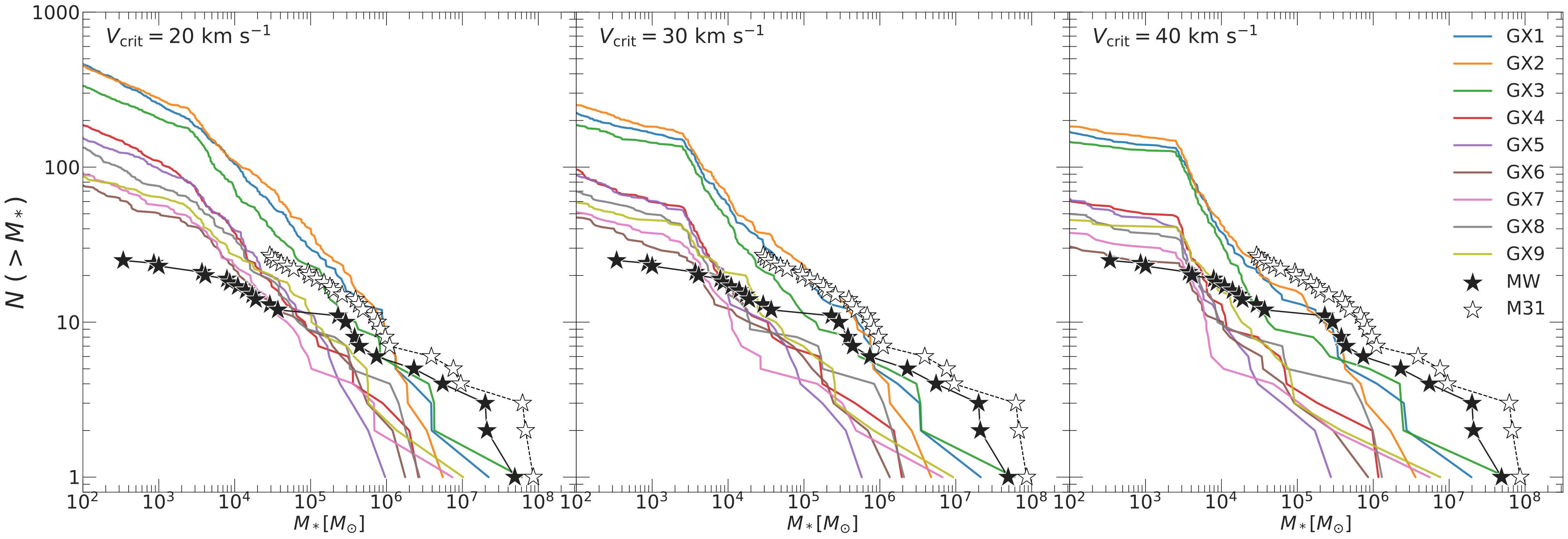 Figure 1
 Figure 2
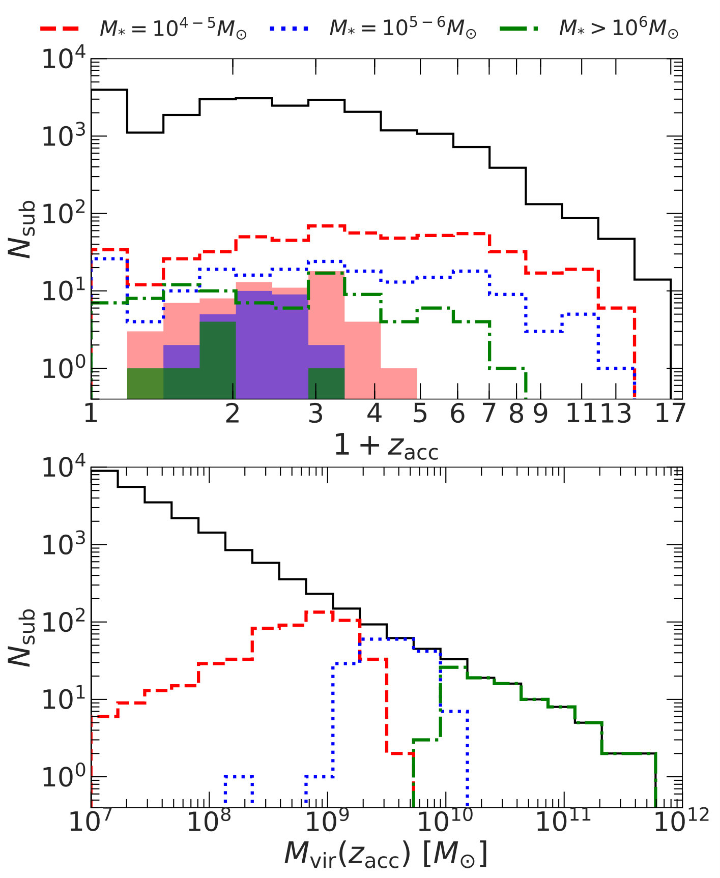 Figure 3
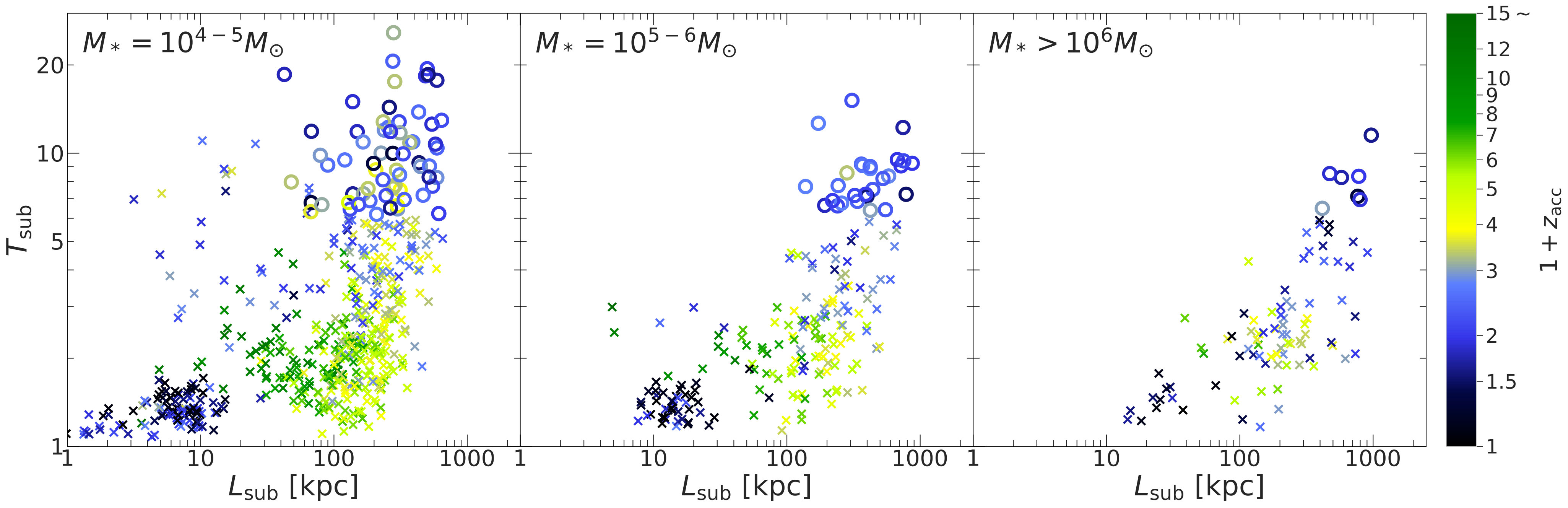 Figure 4
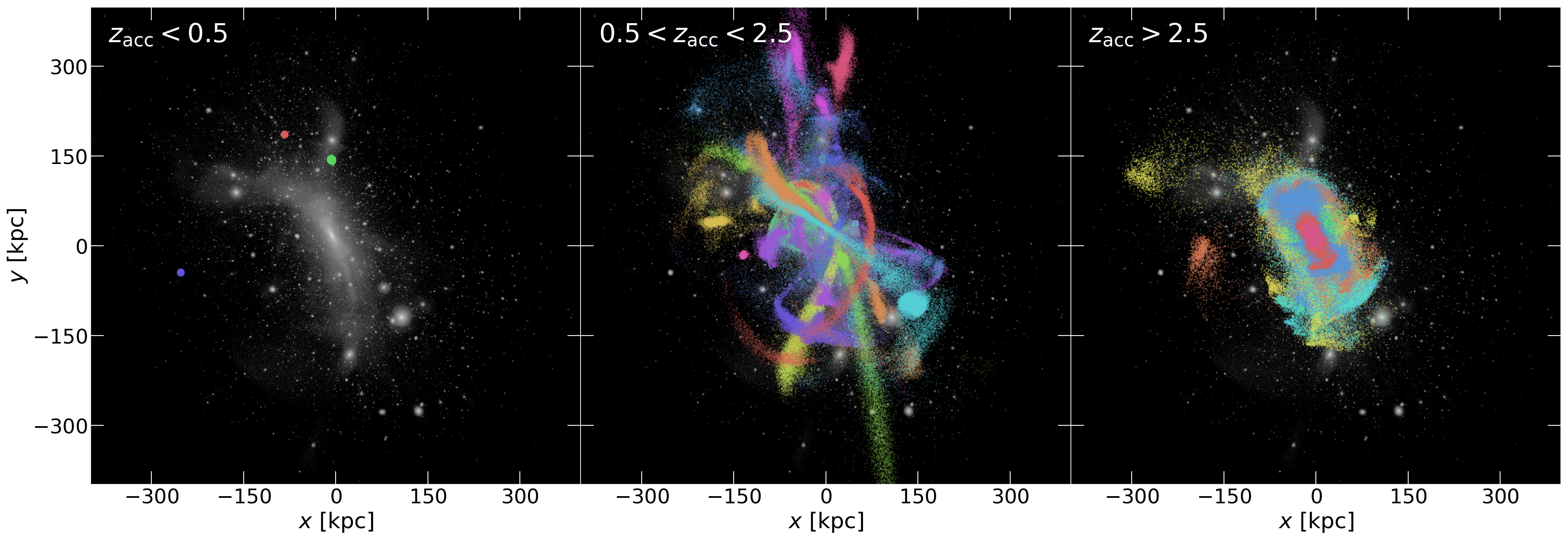 Figure 5
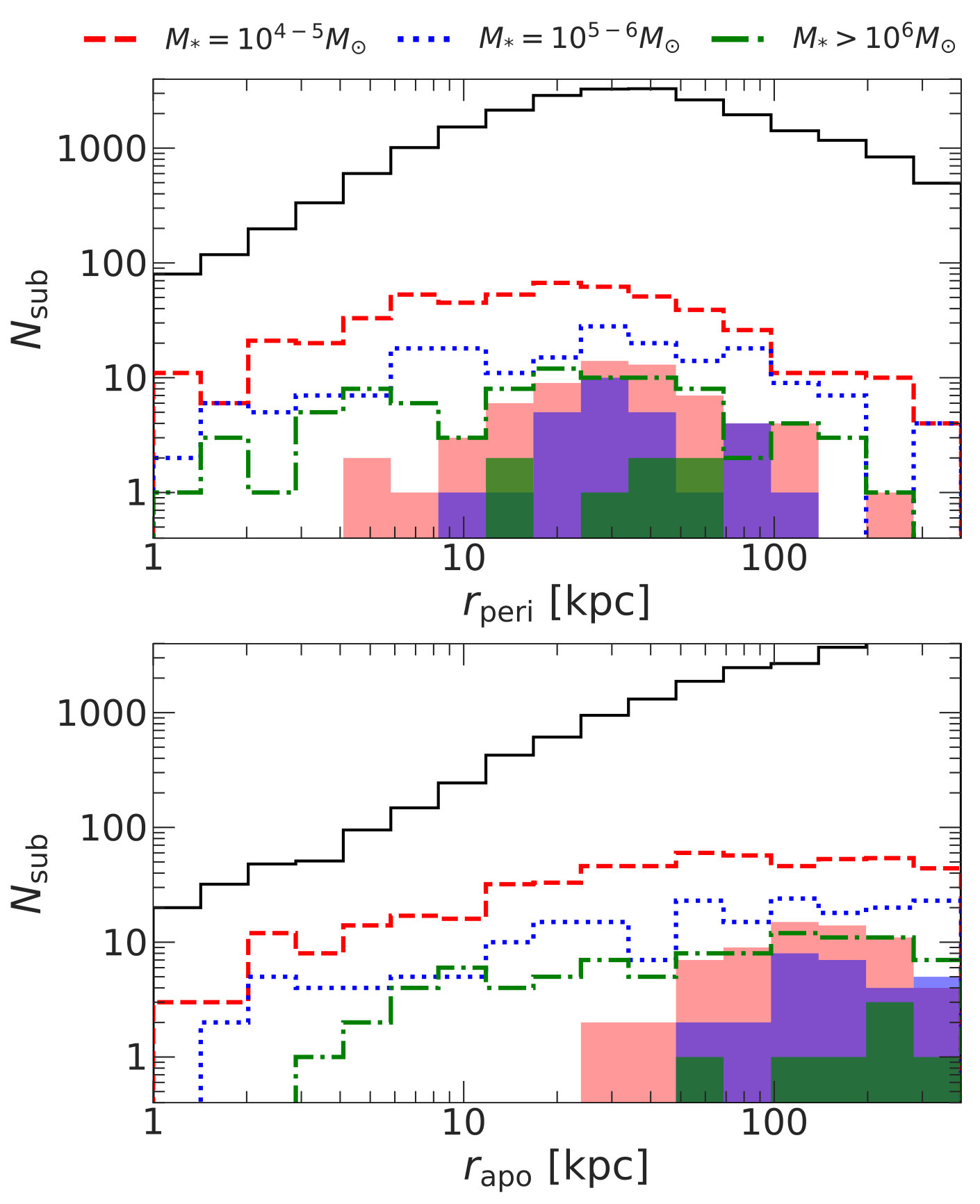 Figure 6
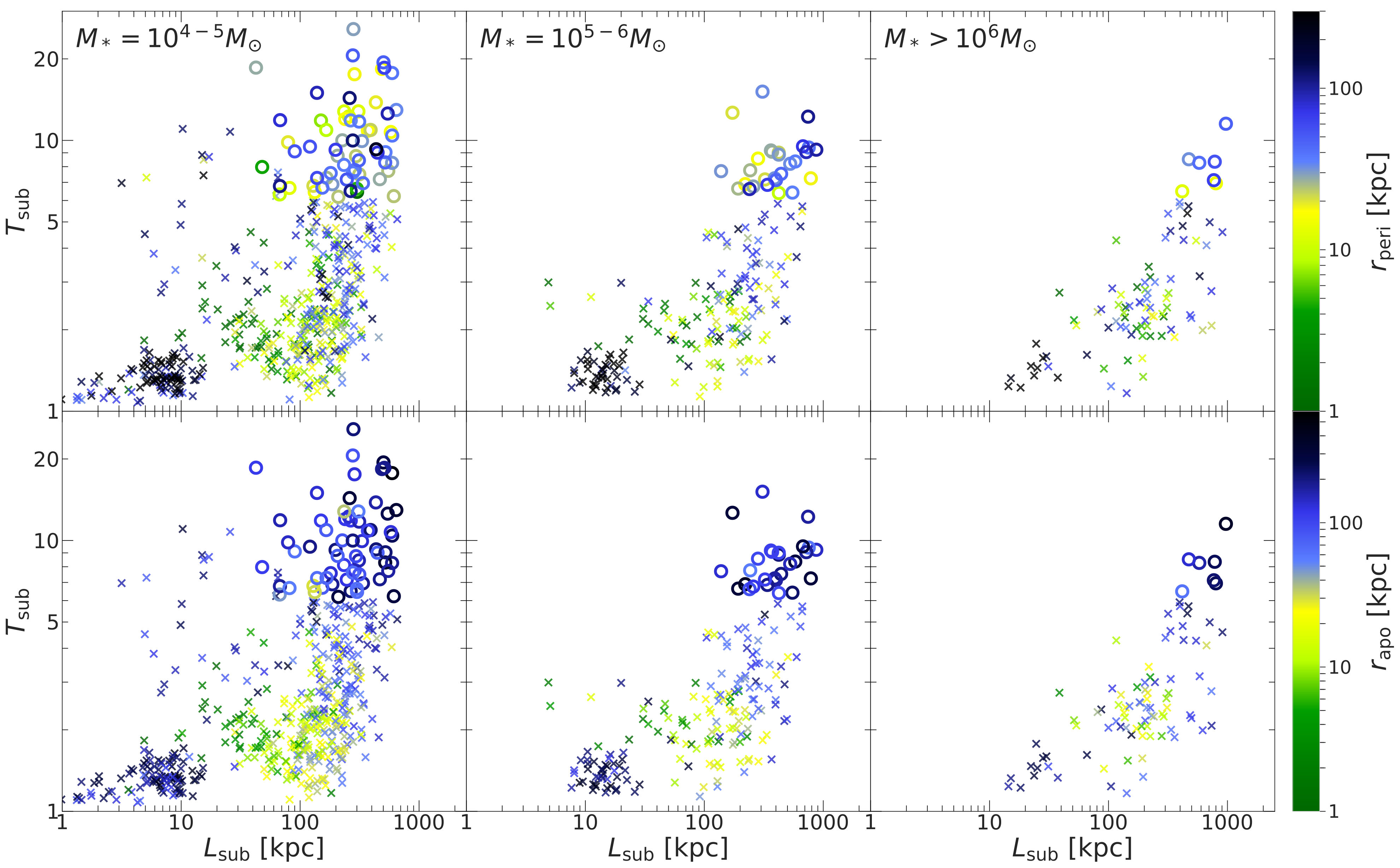 Figure 7
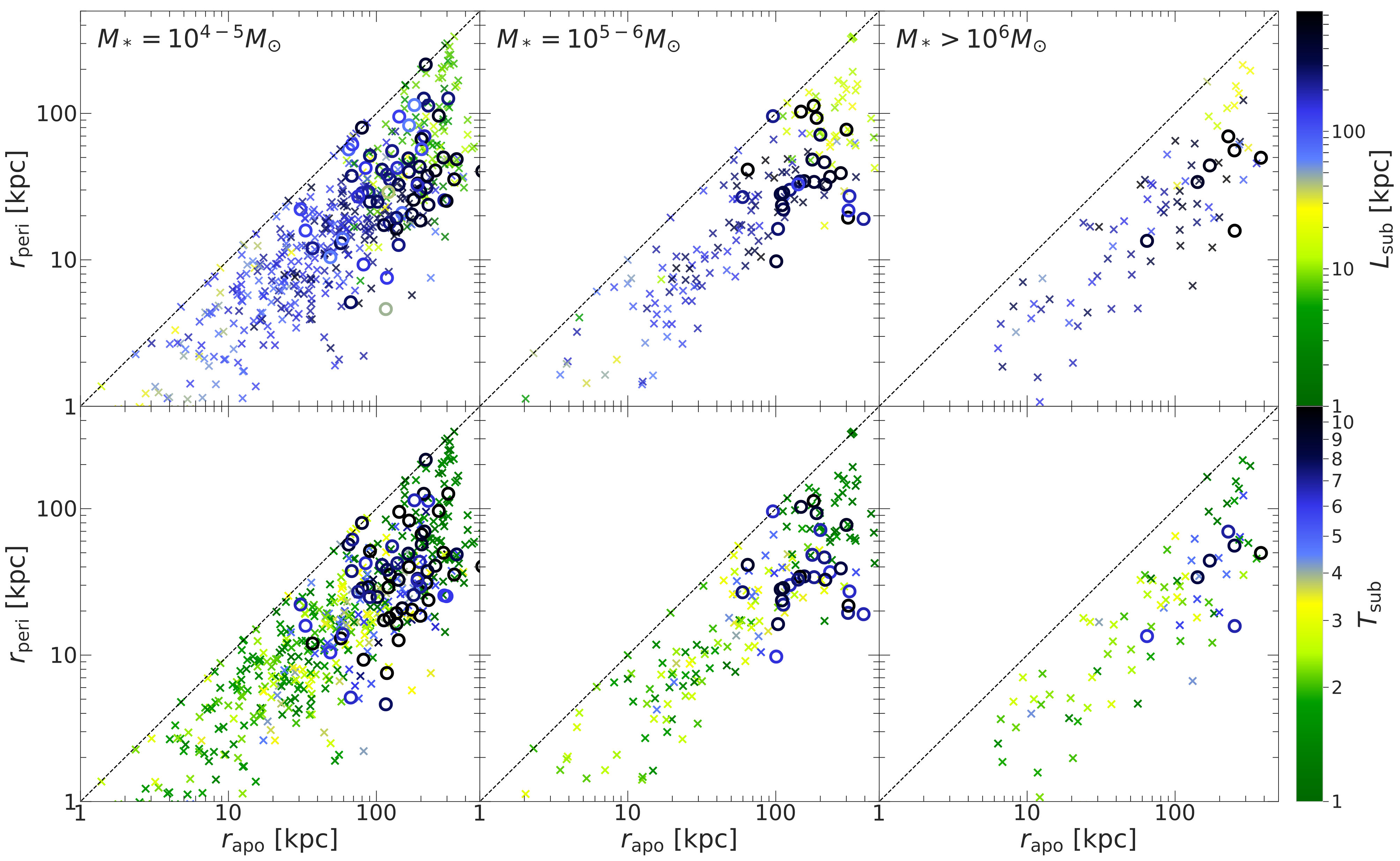 Figure 8
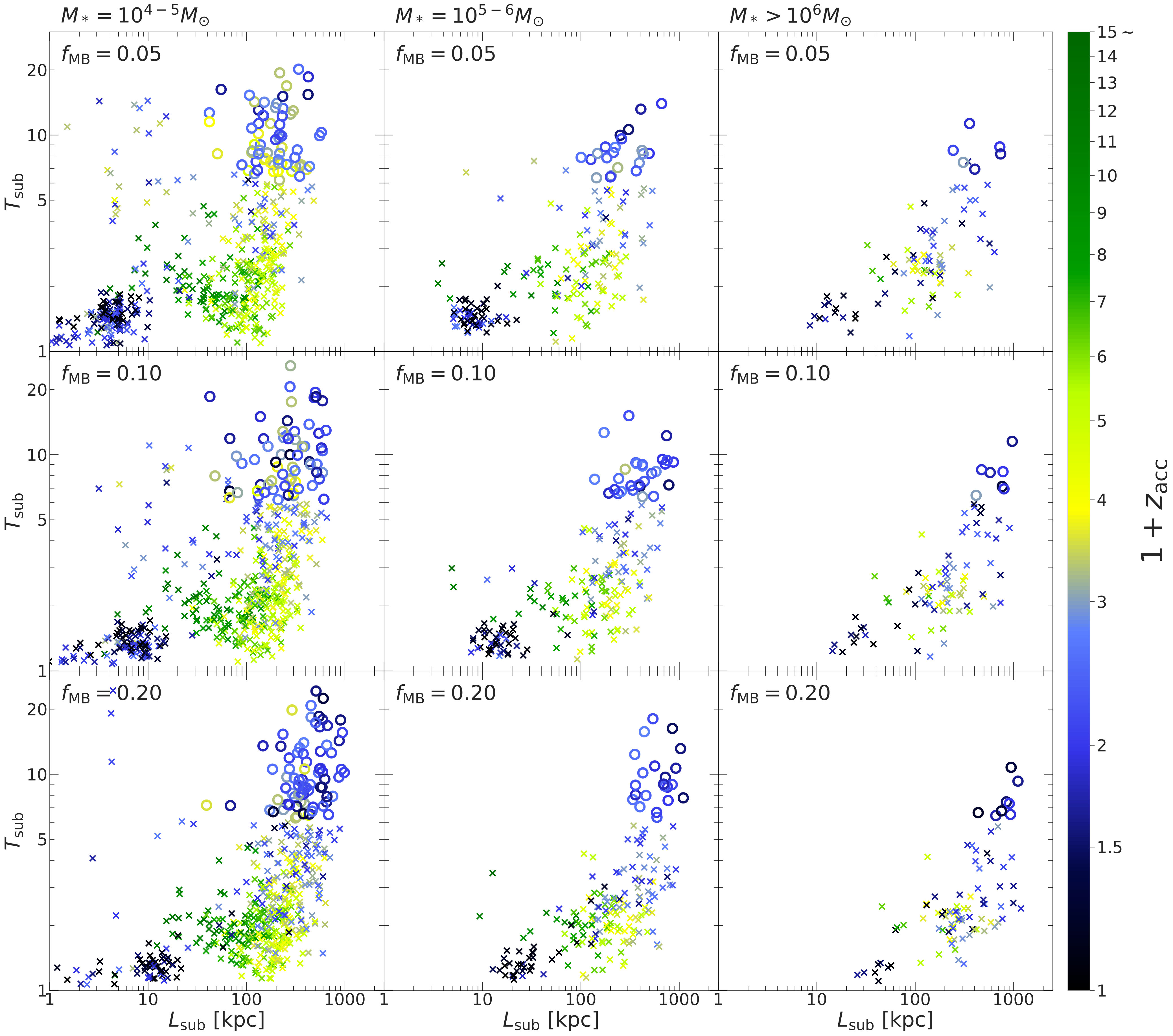 Figure 9
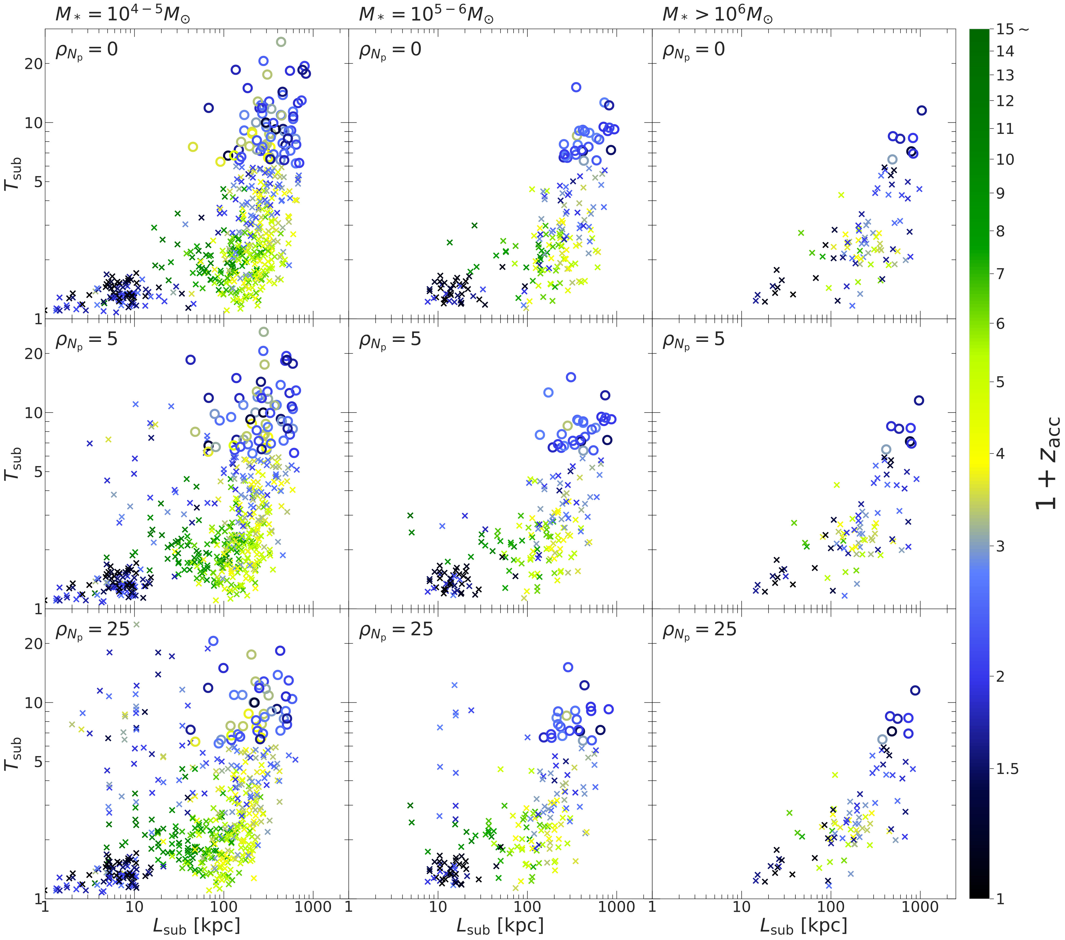 Figure 10
| Name | ||||||
|---|---|---|---|---|---|---|
| [] | ||||||
| GX1 | 6560 | 158 (16) | 52 (8) | 18 (2) | ||
| GX2 | 4956 | 104 (23) | 48 (8) | 20 (2) | ||
| GX3 | 3810 | 86 (11) | 20 (2) | 14 (2) | ||
| GX4 | 2421 | 69 (6) | 19 (0) | 9 (1) | ||
| GX5 | 1853 | 32 (7) | 20 (5) | 7 (0) | ||
| GX6 | 959 | 17 (0) | 11 (0) | 5 (0) | ||
| GX7 | 1135 | 35 (2) | 8 (1) | 6 (0) | ||
| GX8 | 1421 | 26 (2) | 11 (3) | 9 (0) | ||
| GX9 | 1016 | 26 (1) | 11 (0) | 3 (0) |
Peer Reviews
No public reviews on file for this paper yet. If you reviewed it on a platform where reviews are public (OpenReview, ICLR, NeurIPS, ICML), you can paste yours below so the community can read it here.
Videos
No videos yet. Explain this paper in a talk, walkthrough, or lecture? Add one.
Statistical properties of substructures around \textcolorblackMilky Way-sized haloes and their implications for the formation of stellar streams
Yu Morinaga,1 Tomoaki Ishiyama,2 Takanobu Kirihara2 and Kazuki Kinjo1
1Department of Applied and Cognitive Informatics, Chiba University, 1-33, Yayoi-cho, Inage-ku, Chiba 263-8522, Japan
2Institute of Management and \textcolorblackInformation Technologies, Chiba University, 1-33, Yayoi-cho, Inage-ku, Chiba 263-8522, Japan E-mail: [email protected]
(Accepted 2019 May 14. Received 2019 May 10; in original form 2019 January 15)
Abstract
Stellar streams originating in disrupted dwarf galaxies and star clusters are observed around the Milky Way and nearby galaxies. Such substructures are the important tracers that record how the host haloes \textcolorblackhave accreted progenitor galaxies. Based on the cosmological context, we investigate the relationship between structural properties of substructures such as length and thinness at , and orbits of their progenitors. We model stellar components of a large sample of substructures around Milky Way-sized haloes by combining semi-analytic models with a high-resolution cosmological -body simulation. Using the Particle Tagging method, we embed stellar components in progenitor haloes and trace phase-space distributions of the substructures down to . We find that the length and thinness of substructures vary smoothly as the redshift when the host haloes accrete their progenitors. For substructures observed like streams at , a large part of the progenitors is accreted by their host haloes at redshift . Substructures with progenitors out of this accretion redshift range are entirely or less disrupted by and cannot be observed as streams. We also find that the distributions of length and thinness of substructures vary smoothly as pericentre and apocentre of the progenitors. Substructures observed like streams tend to \textcolorblackhave the specific range of and .
keywords:
\textcolorblack galaxies: formation – galaxies: dwarf – galaxies: structure – methods: numerical
††pubyear: 2018††pagerange: Statistical properties of substructures around \textcolorblackMilky Way-sized haloes and their implications for the formation of stellar streams–10
1 Introduction
The standard lambda cold dark matter (CDM) scenario predicts that galaxies are formed via hierarchical mergers of smaller objects over its lifetime (White & Rees, 1978). As a consequence of this merger process, a large number of substructures such as dwarf galaxies and their tidally disrupted remnants including stellar streams are expected to exist around galaxies as fossil records of their accretion events.
Among many kinds of substructures, stellar streams bring especially important clues to \textcolorblackinvestigate galaxy formation. Infalling dwarf galaxies and star clusters into their host galaxies are tidally perturbed, and their stellar components are stripped. These stripped stellar components are elongated and formed tidal tails approximately along the progenitor orbits and observed as structures like “stream” at present (Johnston, Hernquist & Bolte, 1996).
Such streams are the important tracers that record how the host haloes accreted progenitor galaxies because characteristic structural properties of streams should be significantly sensitive to their progenitor orbits \textcolorblack(e.g., Hozumi & Burkert, 2015) and also environments of their host galaxies such as the shape of underlying gravitational potential and interactions with other substructures \textcolorblack(e.g., Johnston et al., 1999; Łokas, Gajda & Kazantzidis, 2013).
So far, a large number of observations have actually discovered substructures including the Sagittarius stream (e.g., Ibata, Gilmore & Irwin, 1994; Ibata et al., 2001b; Majewski et al., 2003), Orphan stream \textcolorblack(Grillmair, 2006; Belokurov et al., 2007; Fardal et al., 2018; Koposov et al., 2019) around the Milky Way (MW), the \textcolorblackGiant Southern Stream in the Andromeda galaxy (M31) (e.g., Ibata et al., 2001a) and many other substructures in nearby galaxies (e.g., Martínez-Delgado et al., 2008; McConnachie et al., 2009). Recent surveys such as the Sloan Digital Sky Survey (SDSS), the Gaia mission (Gaia Collaboration et al., 2016), Dark Energy Survey (DES)(Dark Energy Survey Collaboration et al., 2016), \textcolorblackPan-Andromeda Archaeological Survey (PAndAS) (McConnachie et al., 2009; Martin et al., 2013), \textcolorblackthe Panoramic Survey Telescope and Rapid Response System (Pan-STARRS) (Kaiser et al., 2002) and Subaru Hyper Suprime-Cam (Miyazaki et al., 2006, 2012) have been discovering new faint dwarf galaxies and stellar streams, and measuring \textcolorblacksome properties of a part of individual stars \textcolorblack(e.g., Kalirai et al., 2010; Richardson et al., 2011; Tollerud et al., 2012; Drlica-Wagner et al., 2015; Helmi et al., 2018; Simon, 2018; Shipp et al., 2018; Komiyama et al., 2018; Fu et al., 2018; Homma et al., 2018). These past, ongoing and planning surveys would enable us to characterise the structural properties for plenty of substructures such as the length and thinness in more detail and infer the origin of substructures by comparing with some theoretical models.
To investigate the relationship between structural properties of streams, orbits of their progenitors and environments, various studies have been carried out \textcolorblack(e.g., Ibata et al., 2001b; Johnston, Sackett & Bullock, 2001; Johnston et al., 2008; Majewski et al., 2003; Peñarrubia, McConnachie & Babul, 2006; Peñarrubia et al., 2010; Fardal et al., 2007, 2008, 2013; Sales et al., 2007, 2008; Martínez-Delgado et al., 2008; Varghese, Ibata & Lewis, 2011; Carlberg, 2012; Foster et al., 2014; Miki et al., 2014; Miki, Mori & Rich, 2016; Sandford et al., 2017; Kirihara et al., 2017; Kirihara, Miki & Mori, 2017; Bonaca & Hogg, 2018). Ibata et al. (2001b) suggested that the gravitational potential of the MW must be nearly spherical to reproduce the observed \textcolorblackpositions and \textcolorblackvelocities of stars in the Sagittarius stream. A few gaps found along stellar streams may be caused by a large population of low-mass subhaloes predicted by the CDM model \textcolorblack(Carlberg, 2012; Ibata, Lewis & Martin, 2016; Sandford et al., 2017), which may be a possible explanation for the so called “missing satellite” problem (Klypin et al., 1999; Moore et al., 1999).
For these studies, -body simulations have been extensively used to reproduce observed properties of substructures and to explore the dynamical evolution of them. In many \textcolorblackearlier studies, fixed and spherical gravitational potential of host galaxies \textcolorblackis assumed, and orbits of satellite galaxies are free parameters. However, in the cosmological context, dynamical evolution of substructures are significantly affected by complicated physics such as dynamical friction, multiple interactions with other subhaloes, and evolutionary history of host galaxies, which could not be treated in fixed gravitational potential. Orbital parameters of infalling satellites have some specific distributions (Wetzel, 2011). Consequently, tracing the dynamical evolution of substructures using -body simulations in simple galactic models is insufficient to estimate their origins precisely. Studies based on the cosmological context are highly demanded.
Diemand, Kuhlen & Madau (2007) analysed co-evolution of abundant subhaloes with a host halo formed in their cosmological \textcolorblack-body simulation and showed the mass evolution of subhaloes depends on orbital properties such as pericentre. Warnick, Knebe & Power (2008) examined the formation and evolution of tidal streams originated in cosmological disrupted subhaloes and found correlations between the structures of streams and some properties of progenitor haloes such as infalling masses and orbital parameters. However, the dynamical evolution of subhaloes and dwarf galaxies differ because tidal stripping preferentially occurs in the outer part \textcolorblackof haloes. Besides, they used only one MW-sized host halo, which is not enough to capture the statistics of structural properties of substructures.
To shed light on these issues, we explore the dynamical evolution and structural properties of stellar components of a large sample of substructures within the cosmological context. \textcolorblack In particular, we focus on substructures originating in “dwarf galaxies”, while Carlberg (2018b, a) have explored the formation and evolution of streams originating in globular clusters and their density gaps.
We combine a high-resolution cosmological -body simulation (Ishiyama et al., 2016) with the “Particle Tagging” method to embed stellar components into haloes, which has succeeded to reproduce some observed features of the stellar halo of the MW (e.g., De Lucia & Helmi, 2008). Cooper et al. (2010) have developed an extension method of the Particle Tagging, which is also used to study stellar streams near solar neighbourhood (Gómez et al., 2013). To assign stellar masses to haloes, we use a simple model proposed by Koposov et al. (2009). We aim to investigate the relationship between structural properties of substructures such as length and thinness at , and the orbits of their progenitors in MW-sized haloes.
This paper is organised as follows. In Section 2, we describe the details of our cosmological -body simulation. In Section 3, we explain the analytic models and \textcolorblackthe definition of structural and orbital properties of substructures. In Section 4, we show the results of our statistical analysis of substructures. Finally, we discuss and summarise our results in Section 5.
2 Cosmological -body Simulation
We used a high-resolution cosmological -body simulation conducted by Ishiyama et al. (2016). This simulation consists of dark matter particles in an comoving cubic box. The particle mass is , and the gravitational softening length is . The cosmological parameters are consistent with the observation of the cosmic microwave background obtained by the Planck satellite (Planck Collaboration et al., 2014, 2018), namely, , and . \textcolorblackThe snapshots were stored at the redshifts so that the logarithmic interval . We identified dark matter haloes and subhaloes using ROCKSTAR (Robust Overdensity Calculation using K-Space Topologically Adaptive Refinement) halo/subhalo finder (Behroozi, Wechsler & Wu, 2013). Then we constructed their merger trees using CONSISTENT TREE code (Behroozi et al., 2013), Further details of this simulation are given in Ishiyama et al. (2016).
In this study, we analysed nine MW-sized haloes (GX1-GX9). Their virial mass is between , \textcolorblackwhere the definition of virial mass is given by Bryan & Norman (1998). Their properties such as the virial mass and the virial radius are summarised in Table 1. From their merger trees, we selected progenitor haloes with masses more massive than at redshift when they first pass through the virial radius of the most massive progenitors of MW-sized haloes (so-called “main-branch”). Then, we traced the evolution of these haloes after the redshift . The number of subhaloes in each host halo is listed in Table 1.
After the redshift , most progenitor haloes orbit host haloes as subhaloes. Some of them are disrupted by the gravitational interaction with the host haloes and \textcolorblackcannot be observed at as subhaloes in the merger tree. In the following section, we tag a part of member particles of subhaloes at using the “Particle Tagging” method and regard these particles as the stellar component. By tracing these stellar particles down to , we can analyse the phase space distributions of both \textcolorblacksurviving and disrupted “galaxies” at . \textcolorblackHereafter, including streams, we refer to these objects as “substructures”. In Section 3.4, we categorise them by length and thinness of substructures at into three types, self-bounded subhalo, stream and disrupted substructure. Because there is no consensual and rigid definition of them from the viewpoint of observations, we refer to substrcutures using these three terms as a matter of convenience.
3 Methods
3.1 Particle Tagging
Adopting the “Particle Tagging” method (e.g., Bullock, Kravtsov & Weinberg, 2001; Diemand, Madau & Moore, 2005; Bullock & Johnston, 2005; De Lucia & Helmi, 2008; Cooper et al., 2010) to dark matter only simulations, we can embed stellar components in progenitor haloes and trace their phase space distributions down to . Most stellar components are assumed to be formed in the centre of progenitor haloes until the redshift when they first pass through the virial radius of their host haloes. We tag \textcolorblacka fixed fraction of of the most bound particles of those progenitors at ,111\textcolorblackIf the progenitor halo is a “phantom” halo (Behroozi, Wechsler & Wu, 2013) in the merger tree at , we trace the progenitor back to redshift when it is not phantom and \textcolorblackperform the tagging. and treat these particles as “stellar particles”. Tracing these particles down to , we can investigate the phase space distributions of substructures originating in progenitor haloes. We set by default.
The similar approach was adopted by De Lucia & Helmi (2008). They also used and showed that physical properties such as the metallicity and \textcolorblackthe age of stars in accreted stellar haloes of their model galaxies \textcolorblackwere good agreement with the observed \textcolorblackdata. Besides, they found that observed structural properties of \textcolorblackthe stellar component around the MW were \textcolorblackwell reproduced, reinforcing the effectiveness of the Particle Tagging method. Cooper et al. (2010) have also developed an extension of this method\textcolorblack, which is confirmed to be able to provide an excellent approximation to hydrodynamical simulations (Cooper et al., 2017).
In our study, combining the Particle Tagging method with the higher resolution cosmological -body simulation described in \textcolorblackSection 2, we can resolve substructures such as streams originating in smaller haloes and investigate structural properties of them. Although we used the fraction as a fiducial value, we also compared \textcolorblackthe results with and 0.20, and confirmed that the differences in do not strongly affect statistical results of the relationship between structural properties of substructures and orbits of their progenitors. The detail is given in Appendix A.
3.2 A model to assign stellar masses to haloes
In cosmological -body simulations, MW-sized haloes contain a number of subhaloes as \textcolorblacklisted in Table 1. However, the number of known dwarf galaxies in the MW and M31 is two or three dozens (McConnachie, 2012). This disagreement is known as the so-called “missing satellite” problem (Klypin et al., 1999; Moore et al., 1999). To investigate the statistical properties of visible substructures, it is necessary to assign stellar masses to progenitor haloes in a physically motivated manner.
Photoionising by \textcolorblackthe cosmic UV background radiation sufficiently suppresses the star formation in low-mass haloes with \textcolorblackthe viral temperatures . Such haloes unable to cool the gas and form stars even if sufficient amount of gas exists (Haiman, Rees & Loeb, 1997). To assign stellar masses to subhaloes, we used a model based on this picture proposed by Koposov et al. (2009) that reproduces the distribution of dwarf galaxies observed by the Sloan Digital Sky Survey.
In this model, when the circular velocity of a progenitor halo at \textcolorblackthe reionization epoch \textcolorblack(e.g., Dunkley et al., 2009) is above a critical threshold (corresponding to ), the stellar mass of the progenitor halo is given by Equation (1)
[TABLE]
where and are the virial masses of \textcolorblackthe progenitor halo at and , respectively, and the stellar mass fraction is . In this case, it is assumed that such halo is massive enough to form stars in the pre-reionization era. On the other hand, for a progenitor halo with , the stellar mass is assigned by Equation (2), assuming very low star formation efficiency in the pre-reionization era\textcolorblack,
[TABLE]
In these equations, the suppression of star formation occurs for haloes with the circular velocity below a critical value after the reionization, based on cosmological hydrodynamical simulations (e.g., Gnedin, 2000; Hoeft et al., 2006; Okamoto, Gao & Theuns, 2008) , and thus resulting stellar masses are significantly affected by the choice of . Gnedin (2000) proposed the critical circular velocity , but lower critical values were \textcolorblacksuggested by Hoeft et al. (2006) and Okamoto, Gao & Theuns (2008). We \textcolorblackvary and select an appropriate value so that the observed stellar mass function of dwarf galaxies \textcolorblackis reproduced well.
Figure 1 shows the cumulative number of subhaloes at (not substructures) in nine MW-sized host haloes (GX1-GX9) as a function of stellar mass, for models of and . Filled and open symbols are the distributions of the observed dwarf galaxies in the MW and M31 (McConnachie, 2012), \textcolorblackrespectively. \textcolorblackKoposov et al. (2009) adopted this model and successfully reproduced the distribution of the observed stellar mass function of dwarf galaxies excluding Large/Small Magellanic Clouds. \textcolorblackIn the same manner, we also plot the stellar mass function of the MW and M31 excluding the Magellanic Clouds, M33 and M32.
Subhaloes with \textcolorblacklower stellar masses () are more abundant than observed dwarf galaxies of both the MW and M31 regardless of . One of the \textcolorblackreasons is that it is hard to observe such \textcolorblackultra faint dwarf galaxies \textcolorblackdue to the detection limit. However a part of such faint dwarf galaxies would be discovered by ongoing deep imaging surveys by Subaru Hyper Suprime-Cam (e.g. Homma et al., 2016, 2018). Another reason is that the suppression of star formation in low-mass haloes might be insufficient in this model. \textcolorblack Because such dwarf galaxies are too faint, we only analyse substructures with in this study.
Thus, this disagreement of the number of low stellar mass dwarf galaxies \textcolorblackdoes not change our conclusion.
\textcolor
blackAlthough subhaloes with the stellar mass are not found in any host haloes in our simulation, \textcolorblacksuch satellites are observed in the MW and M31 such as Large/Small Magellanic Clouds, \textcolorblackM33 and M32. Recent cosmological simulations have also shown that MW-sized haloes to host such massive satellites are rare (Boylan-Kolchin, Besla & Hernquist, 2011; Busha et al., 2010). Therefore, this disagreement does not affect the statistical properties of substructures. When we exclude these dwarf galaxies, the agreement between our model and the observation \textcolorblackbecomes better for and . Hereafter, we use , \textcolorblackand the number of substructures (not subhaloes at ) with the critical threshold in each host halo is listed in Table 1.
3.3 Orbital parameters
To analyse orbital histories of subhaloes and how they relate to the properties of substructures, we quantify the pericentre and apocentre of subhaloes. Wetzel (2011) explored orbital properties of infalling satellites and reported \textcolorblacktheir dependence on the host and satellite masses and redshift. They calculated the orbital circularity and pericentre by the two-body approximation (host and satellite haloes). This procedure would be valid for infalling satellites. However, after , actual orbital properties such as pericentre and apocentre evolve via dynamical friction, tidal disruption, and multiple interactions between subhaloes. Therefore, the two-body approximation is not accurate enough to describe \textcolorblackthe orbital properties.
To calculate the pericentre and apocentre of subhaloes more accurately, we trace their orbits from to or \textcolorblackthe redshift when they are entirely merged with their host haloes. Then we define the pericentre (apocentre) as the smallest value in local minima (maxima) of the radial distance of subhaloes. When subhaloes do not experience any pericentre or apocentre passages, we define the pericentre as the smallest radial distance and the apocentre as the largest radial distance after so that we can quantify \textcolorblackthe orbital properties.
3.4 Quantifying structural properties of substructures
We characterise structural properties of substructures at and explore the relationship between them and the orbits of progenitors. We quantify them with two characteristic parameters, length , and thinness .
3.4.1 Definition of the length of substructures
\textcolor
black We define the length of substructures as follows. At first, we perform the Principal Component Analysis (PCA) for the stellar particles of substructures in the three-dimensional coordinate. The spatial coordinate is transformed to the new coordinate (PC1-3). Then, we define the length of a substructure as the sum of physical distances of two stellar particles that lie furthest along the PC1 axis to the centre of the substructure. To exclude outliers, we count the number of stellar particles in the substructure along the PC1 axis at intervals of and remove particles in the region whose number of particles is below five in calculating the length. In this case, the threshold of the outlier removal step is represented by . Although we use as a fiducial value throughout this paper, we also compare the results of the structural properties of substructures with in Appendix B, which indicates that statistical results are insensitive to the choice of .
3.4.2 Definition of the thinness of substructures
To quantify the thinness of substructures, we apply a similar method proposed by Sandford et al. (2017). \textcolorblackWe perform PCA for the stellar particles of substructures in the three-dimensional coordinate, and each stellar particle (denoted by ) is represented by principal components scores . The PC1 (PC3) scores have the largest (smallest) variance in the three.
Using these variances, we define the thinness as
[TABLE]
where is the number of stellar particles in the substructure. In other words, represents the ratio of the standard deviation of PC1 to PC3. For example, a substructure with high- is elongated along PC1 and would be observed like a stream at . On the other hand, a substructure with low- distributes three-dimensionally, which means it is entirely disrupted or is not much tidally affected.
3.4.3 Definition of the stream
We consider that substructures with large values of the length and thinness can be observed as stellar streams. In this paper, we refer to substructures with and at as streams, where is the virial radius of the progenitor halo at . In the case of massive substructures, is naturally high even if they are not tidally disrupted. To pick up tidally elongated substructures, we define the stream by , which represents the relative disruption of substructures. Entirely disrupted substructures or slightly disrupted substructures are not categorised as streams in this definition because such substructures have smaller values of .
4 Results
4.1 Distribution of length and thinness
Figure 2 shows the distributions of length and thinness of \textcolorblackall substructures with stellar mass ranges of and \textcolorblackin nine MW-sized haloes (GX1-GX9). The distribution of the length shows a bimodality regardless of the stellar mass range. The first peak at short length around kpc originates from less disrupted substructures. The second peak at the long length from to originates from entirely disrupted substructures. The first peak slightly shifts towards the long length with increasing the stellar mass because the size of progenitor haloes becomes larger. On the other hand, the second peak is almost unchanged.
The distribution of thinness shows that the number of substructures decreases as the thinness increases\textcolorblack, and \textcolorblackpeaks at around . This trend is also seen in substructures with any stellar mass ranges, indicating that the highly elongated substructures are quite rare and a large part of substructures is not observed as streams at .
4.2 Relation between length \textcolorblack, thinness \textcolorblack and accretion redshift
To explore the accretion histories of substructures around MW-sized haloes at , we plot the distributions of and masses of their progenitor haloes at in Figure 3. From the overall distribution of , the number of progenitors with mass tends to be decreasing with increasing redshift from , just because haloes more massive than this value are not enough formed (the half mass formation epoch of such haloes is (Ishiyama et al., 2015)). These trends propagate substructures with the stellar mass . The distributions of streams are clearly different from the overall distribution of substructures. A large part (approximately ) of the streams is accreted by their host haloes within . On the other hand, only of all substructures is accreted within this redshift range.
As shown in the bottom panel of Figure 3, the mass distribution of substructures with the progenitor mass approximately follows a power law. However, those within a certain range of stellar masses differ depending on the range. The substructures with the stellar mass ranges of and approximately correspond to the progenitor haloes with the mass ranges of and , respectively. Almost all the progenitor haloes with mass have relatively massive stellar components (). On the other hand, in low-mass progenitor haloes, the star formation is strongly suppressed in our model due to \textcolorblackthe photoionised heating by the cosmic UV background \textcolorblackradiation. Therefore, a large part of low-mass progenitor haloes with the mass below at \textcolorblackis excluded in our analysis.
Figure 4 shows the distributions of length and thinness at for substructures with the stellar mass ranges of and . The length tends to get longer, and the thinness tends to get slightly smaller for \textcolorblacksubstructures with more stellar \textcolorblackmasses as shown in Figure 2. The length and thinness vary smoothly as the accretion redshift . A large part of substructures with exists in the region with the short length () and \textcolorblackthe small thinness (), indicating that these substructures are less affected by tidal forces from their host haloes because of recent accretion (small ). On the other hand, a large part of substructures with is strongly perturbed by the tidal force and has the long length. The typical length of substructures at is about 1-10 kpc, increased by a factor of approximately 1-50 until . These substructures show a clear correlation between and . The thinness is decreasing with increasing . In particular, substructures with the long length () and \textcolorblackthe large thinness (), which are defined as streams in this work, give a specific redshift range of as shown in Figure 3.
Toward higher accretion redshift (), the thinness of substructures tend to become gradually smaller in any stellar mass ranges. These substructures suffer from strong tidal forces, can be entirely disrupted by and cannot be observed as streams. These trends are highlighted in Figure 5, which shows the distributions of stellar particles of substructures with different accretion redshift ranges of , and . This figure visualises that the different accretion redshift \textcolorblackgives the stark difference in structural properties of substructures.
Substructures with the accretion redshift are less disrupted, and their stellar particles distribute compactly. Thus, their length and thinness tend to be short and small at . In the case of substructures with , most of them are entirely disrupted, and their stellar particles are scattered vastly at . As a consequence, their length stays long, and thinness tends to become smaller with increasing accretion redshift. On the other hand, substructures with characteristic accretion redshift show a variety of structures at . Some of them are largely disrupted and formed stream-like structures. Additionally, there are also some substructures that are less or entirely disrupted. Therefore, these substructures with the characteristic accretion redshift show some scatters in Figure 4. These scatters can also \textcolorblackbe resulted from the variation of orbital properties of their progenitor haloes.
4.3 Relation between length, thinness and orbital parameters
In this section, we investigate the relation between the properties of substructures and orbital parameters. Figure 6 shows the distributions of pericentre and apocentre for progenitors of substructures and streams with the stellar mass ranges of and .
The distribution of the pericentre of substructures with peaks at around kpc, implying that the progenitor haloes with smaller tend to be entirely merged with their host haloes by . This peak is also seen in the substructures with the stellar mass of , however, is less prominent. The progenitor haloes experience pericentre passages in a rather wide range of . On the other hand, a large part of progenitor haloes of streams \textcolorblackexperiences pericentre passages in a shorter and narrow range of , and the peak is more prominent.
The number of substructures with increases with increasing apocentre. This dependence is weakened in the substructures with stellar mass of . \textcolorblackIt means that numerous lower stellar mass haloes are just infalling into the host haloes. On the other hand, the apocentre of a large part of streams distributes in . The distributions of pericentre and apocentre of streams show the stark difference from the overall distribution of substructures.
To see the relation between the properties of substructures and \textcolorblackthe orbital parameters, we plot the distribution of length versus thinness as \textcolorblackfunctions of orbital parameters for substructures with stellar mass ranges of \textcolorblackand in Figure 7. As well as the distribution of shown in Figure 4, the distributions of the length and thinness vary smoothly as the pericentre and apocentre in any stellar mass ranges.
Substructures whose progenitor haloes have larger pericentre () tend to exist in the rather narrow region of length and thinness plane ( and ). These substructures are less tidally disrupted by host haloes until , corresponding to substructures with lower . On the other hand, a large part of substructures with smaller pericentre () is strongly perturbed by tidal forces of host haloes, gets their length longer, and shows a considerable variation of thinness. Notably, the substructures observed like streams tend to \textcolorblackoriginate in progenitor haloes with a specific range of pericentre of , corresponding to \textcolorblackthe substructures with as shown in Figure 4.
For substructures with smaller pericentre (), their thinness becomes smaller with decreasing pericentre although there is some scatter. These results suggest that progenitor haloes of such substructures experience multiple pericentre passages and are entirely disrupted or make multiple streams because their accretion redshift \textcolorblacktends to be higher than as shown in Figure 4. The higher means that the size of host haloes at is smaller than their counterparts at and orbital decay due to dynamical friction acts more effectively, contributing the smaller pericentre.
These overall trends are common in any stellar mass ranges, and similar trends \textcolorblackare also seen in the distribution of length versus thinness as \textcolorblacka function of apocentre. Substructures observed like streams tend to have apocentre above , which is slightly smaller than the value that less disrupted substructures have ( and ).
Figure 8 gives another look of the relation between the properties of substructures and \textcolorblackthe orbital parameters, \textcolorblackwhich is the pericentre versus apocentre as a function of length and thinness. The pericentre and apocentre of progenitor haloes distribute in wide ranges from a few to and correlate with each other. As also seen in Figure 7, the distributions of length and thinness of substructures vary as pericentre and apocentre. It is clear that substructures observed like streams are concentrated in the narrow region of the pericentre and apocentre plane \textcolorblackof and . These trends are shown in any stellar mass ranges.
From these results, we can infer the evolution of structural properties of substructures in terms of \textcolorblackthe accretion redshift and \textcolorblackthe orbital parameters. We can clearly see that moderate tidal effects from host haloes are necessary to form streams. Substructures with higher accretion redshift () suffer from strong tidal forces and orbital decay, or have smaller host haloes at , resulting in smaller pericentre and apocentre. Such substructures experience multiple pericentre passages and are entirely disrupted or make multiple streams, making length longer and thinness smaller. Substructures with lower accretion redshift () are less affected by the tidal forces and keep larger pericentre and apocentre \textcolorblackuntil , and also keep their gravitationally bound structures.
5 Discussions and Summary
In this study, we have investigated the relationship between structural properties of substructures and orbits of their \textcolorblackprogenitors around MW-sized haloes. Using a high-resolution cosmological -body simulation and the Particle Tagging method, we have explored the dynamical evolution of a large sample of substructures based on cosmological context more precisely than previous similar studies using -body simulations and simple galactic models.
We have characterised structural properties of substructures using two quantities, length and thinness , and have found that both quantities at vary smoothly as accretion redshift when their progenitor haloes are accreted onto the host haloes. In the case of substructures with , their length and thinness tend to be short and small ( and ). On the other hand, a large part of substructures (approximately 90%) observed like “streams” at \textcolorblackis accreted at the specific accretion redshift range . Toward higher accretion redshift (), the thinness of substructures \textcolorblacktends to become smaller due to \textcolorblackbeing entirely disrupted by tidal forces, and hence they cannot be observed as streams. We have confirmed this trend in substructures with any stellar mass ranges \textcolorblackand .
The \textcolorblackdistributions of length and thinness of substructures also vary as pericentre and apocentre of their progenitor haloes. Substructures whose progenitor haloes experienced larger pericentre passage tend to be less disrupted at . On the other hand, a large part of largely disrupted substructures originates in progenitor haloes with . Notably, substructures observed like streams tend to be concentrated in the specific range of and .
\textcolor
black Throughout this paper, we do not take the effect of baryonic physics into account. Some substructures with small pericentre can be efficiently destroyed by disk shocking (e.g. D’Onghia et al., 2010; Sawala et al., 2017; Garrison-Kimmel et al., 2017; Kelley et al., 2018) and may not be observed as streams. However, in our results, streams tend to have the specific range of and experience a few pericentre passages after because of their specific accretion redshift range . Therefore, baryonic physics should not strongly affect our statistical properties of streams. In the case of substructures that are strongly affected by baryonic physics, their pericentre distances must be small (). In addition, from Figure 4 and Figure 7, such substructures have high- and most of them are already categorised as disrupted substructures. Therefore, considering baryonic physics, these substructures may be more largely disrupted and the type of them does not change.
\textcolor
blackAlthough the definition of stream adopted in this study might be seemed arbitrary, there is no consensual definition of observed streams. It should be stressed that our conclusion is insensitive to the choice of the lower boundary of because the thinness of substructures varies smoothly as the orbital properties of progenitor haloes.
Our studies have been highlighting that moderate tidal effects resulted from such as specific ranges of pericentre, apocentre and of progenitor haloes are necessary to form stream-like substructures at . Note that we have focused on the physical origin of structural properties of substructures and have not pursued the connection with “observed” properties. This is beyond the scope of this paper and will be addressed in future studies.
Acknowledgements
\textcolor
blackWe thank the anonymous referee for his/her valuable comments. We thank Miho N. Ishigaki, Kohei Hayashi and Tomoyuki Hanawa for fruitful discussions and comments. Numerical computations were partially carried out on the K computer at the RIKEN Advanced Institute for Computational Science (Proposal numbers hp150226, hp160212, hp170231, hp180180), Aterui and Aterui II supercomputer at Center for Computational Astrophysics, CfCA, of National Astronomical Observatory of Japan. This work has been supported by MEXT as “Priority Issue on Post-K computer” (Elucidation of the Fundamental Laws and Evolution of the Universe) and JICFuS. We thank the support by MEXT/JSPS KAKENHI Grant Number 17H04828, \textcolorblack17H01101 and 18H04337.
Appendix A Comparing structural properties with different most-bound fraction for the Particle Tagging method
We compare statistics in structural properties of substructures using three most-bound fraction \textcolorblackand for the Particle Tagging method. The most-bound fraction is a free-parameter, which determines the fraction of stellar particles to dark matter particles of a progenitor halo at the accretion redshift . Therefore, the \textcolorblacknumber of stellar particles in haloes increases with increasing . The detail is given in Section 3.1.
Figure 9 is the same as Figure 4. However, top, middle and bottom panels show the distributions of length and thinness of substructures at for \textcolorblackand , \textcolorblackrespectively. The distributions of the length tend to become slightly longer with increasing . It is expected that tidal stripping preferentially occurs in the outer part of subhaloes, and hence the stellar particles of substructures are more vastly scattered in the model using \textcolorblackgreater . However, overall distributions of length and thinness are not so changed regardless of \textcolorblackthe adopted . Especially, for largely disrupted substructures with , their length and thinness vary smoothly as for any given . For less disrupted substructures with and , their number with increases with decreasing , especially in the low stellar mass range of . This is because that stellar components tagged with \textcolorblacksmaller are more tightly bound and less affected by tidal interactions with host haloes.
From these results, we can conclude that our statistical results of the relationship between \textcolorblackthe structural properties of substructures and \textcolorblackthe orbits of their progenitors are insensitive to the choice of .
Appendix B Comparing structural properties with different threshold for outlier removal step of quantifying
\textcolor
black We compare statistics in structural properties of substructures using three thresholds and for outlier removal step of quantifying length of substructures. The definition of the threshold is described in Section 3.4.1.
\textcolor
black Figure 10 is the same as Figure 4. However top, middle and bottom panels show the distributions of length and thinness of substructures at for and , respectively. The distributions of length tend to become slightly shorter with increasing , however, overall trends of the distributions are not changed in any . Therefore, we conclude that our statistical results of the structural properties of substructures are insensitive to the choice of .
The reference list from the paper itself. Each links out to its DOI / PubMed record.
- 1Behroozi, Wechsler & Wu (2013) Behroozi P. S., Wechsler R. H., Wu H.-Y., 2013, Ap J, 762, 109
- 2Behroozi et al . (2013) Behroozi P. S., Wechsler R. H., Wu H.-Y., Busha M. T., Klypin A. A., Primack J. R., 2013, Ap J, 763, 18
- 3Belokurov et al . (2007) Belokurov V. et al., 2007, Ap J, 658, 337
- 4Bonaca & Hogg (2018) Bonaca A., Hogg D. W., 2018, Ap J, 867, 101
- 5Boylan-Kolchin, Besla & Hernquist (2011) Boylan-Kolchin M., Besla G., Hernquist L., 2011, MNRAS, 414, 1560
- 6Bryan & Norman (1998) Bryan G. L., Norman M. L., 1998, Ap J, 495, 80
- 7Bullock & Johnston (2005) Bullock J. S., Johnston K. V., 2005, Ap J, 635, 931
- 8Bullock, Kravtsov & Weinberg (2001) Bullock J. S., Kravtsov A. V., Weinberg D. H., 2001, Ap J, 548, 33