Age determination for 269 $Gaia$ DR2 Open Clusters
D. Bossini, A. Vallenari, A. Bragaglia, T. Cantat-Gaudin, R. Sordo, L., Balaguer-N\'u\~nez, C. Jordi, A. Moitinho, C. Soubiran, L. Casamiquela, R., Carrera, and U. Heiter

TL;DR
This study utilizes Gaia DR2 data and Bayesian isochrone fitting to accurately determine ages, distances, and extinctions for 269 open clusters, enhancing our understanding of Galactic disk properties.
Contribution
It introduces an automated Bayesian method for precise age and parameter estimation of open clusters using Gaia data, improving upon previous techniques.
Findings
Derived ages, distances, and extinctions for 269 open clusters.
Selected low-reddening, non-very young clusters for reliable age estimation.
Demonstrated the effectiveness of Gaia data combined with Bayesian isochrone fitting.
Abstract
. Gaia Second Data Release provides precise astrometry and photometry for more than 1.3 billion sources. This catalog opens a new era concerning the characterization of open clusters and test stellar models, paving the way for a better understanding of the disc properties. . The aim of the paper is to improve the knowledge of cluster parameters, using only the unprecedented quality of the Gaia photometry and astrometry. . We make use of the membership determination based on the precise Gaia astrometry and photometry. We apply anautomated Bayesian tool, BASE-9, to fit stellar isochrones on the observed G, GBP, GRP magnitudes of the high probability member stars. . We derive parameters such as age, distance modulus and extinction for a sample of 269 open clusters, selecting only low reddening objects and discarding very young clusters, for which techniques…
Click any figure to enlarge with its caption.
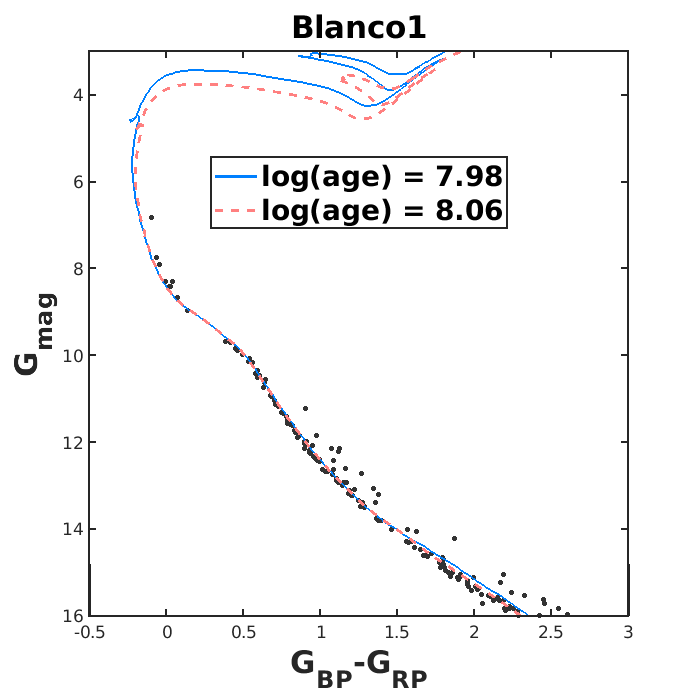 Figure 1
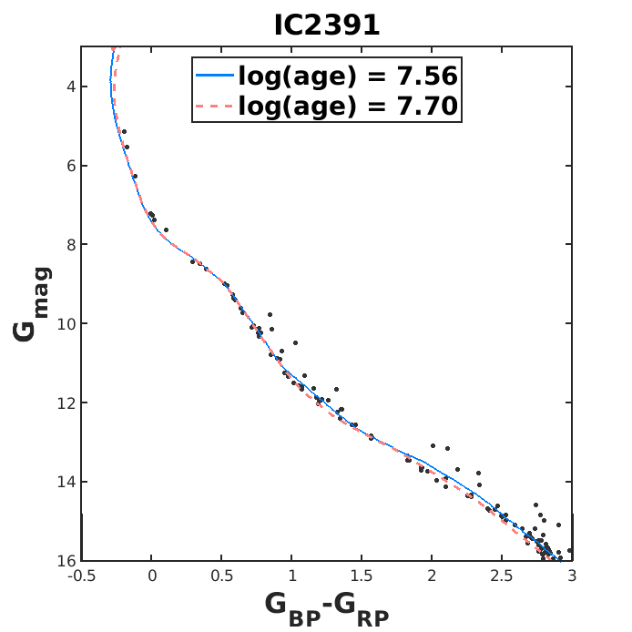 Figure 2
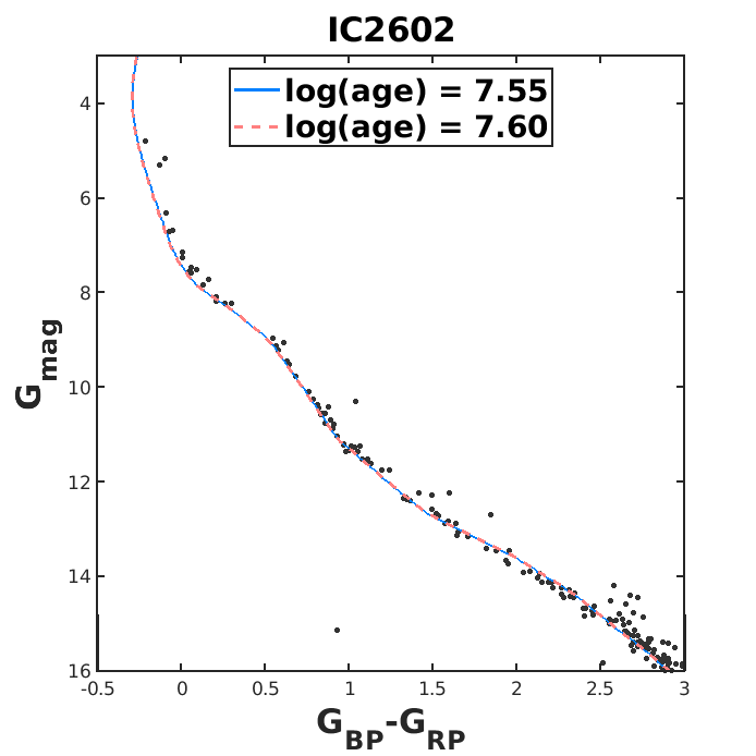 Figure 3
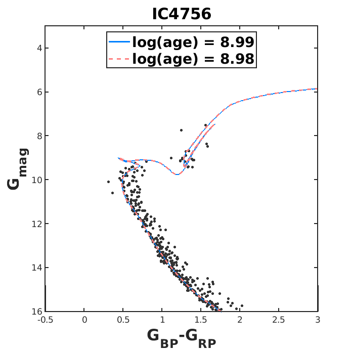 Figure 4
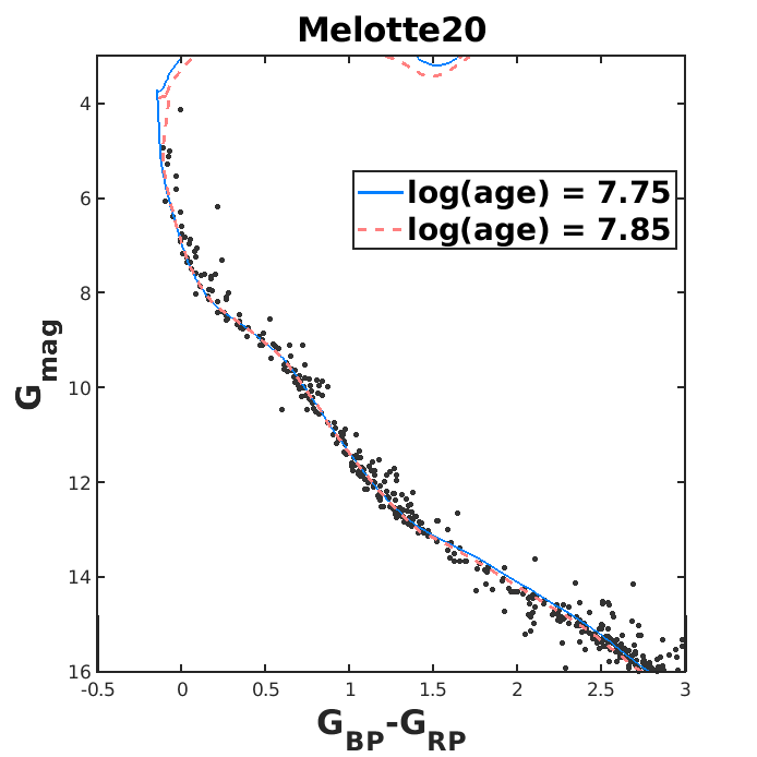 Figure 5
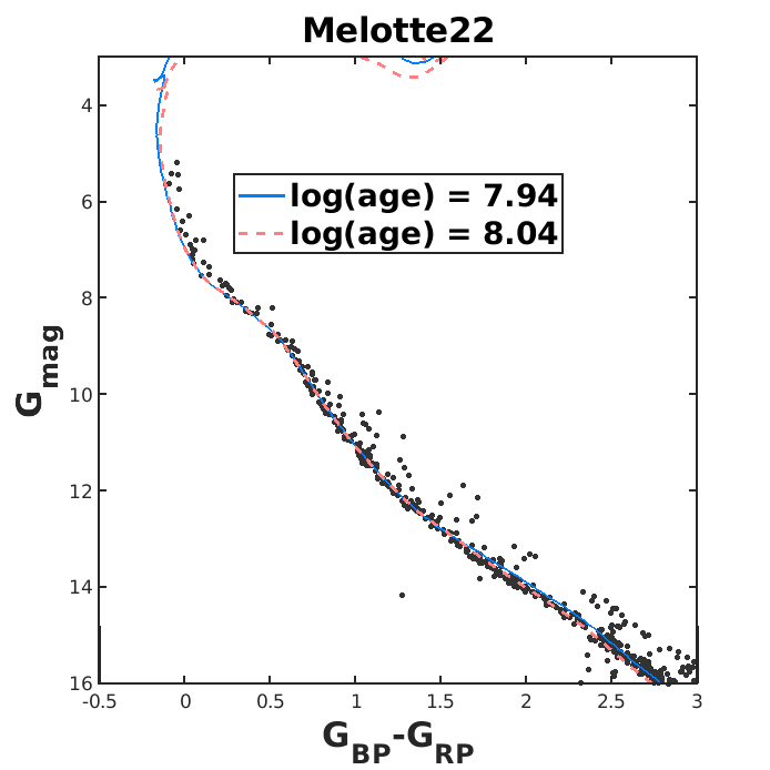 Figure 6
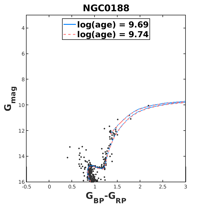 Figure 7
 Figure 8
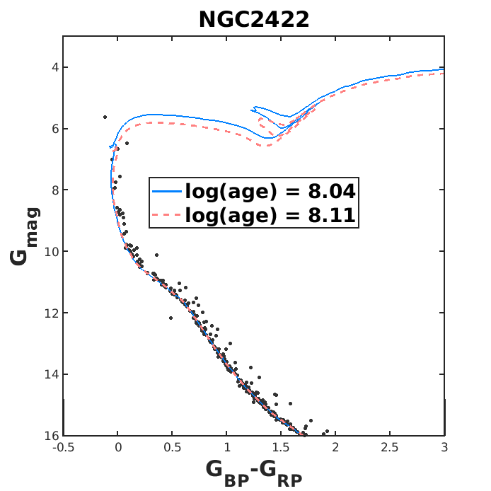 Figure 9
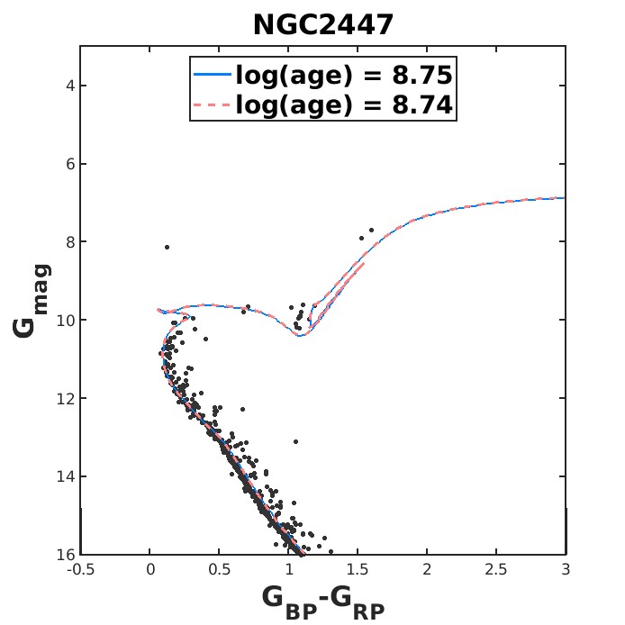 Figure 10
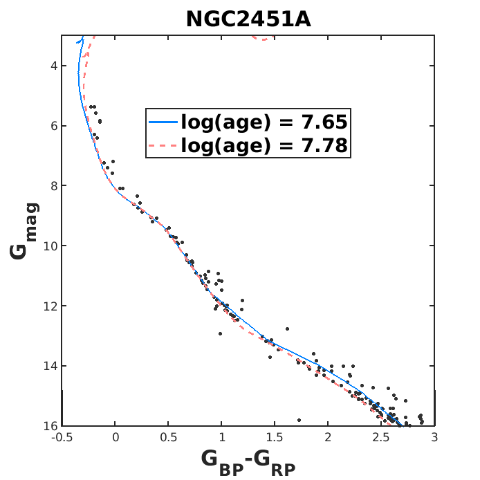 Figure 11
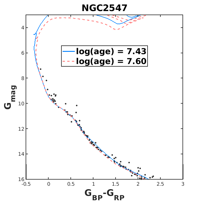 Figure 12
 Figure 13
 Figure 14
 Figure 15
 Figure 16
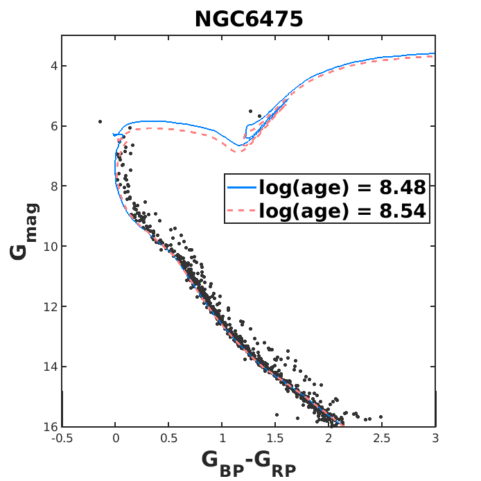 Figure 17
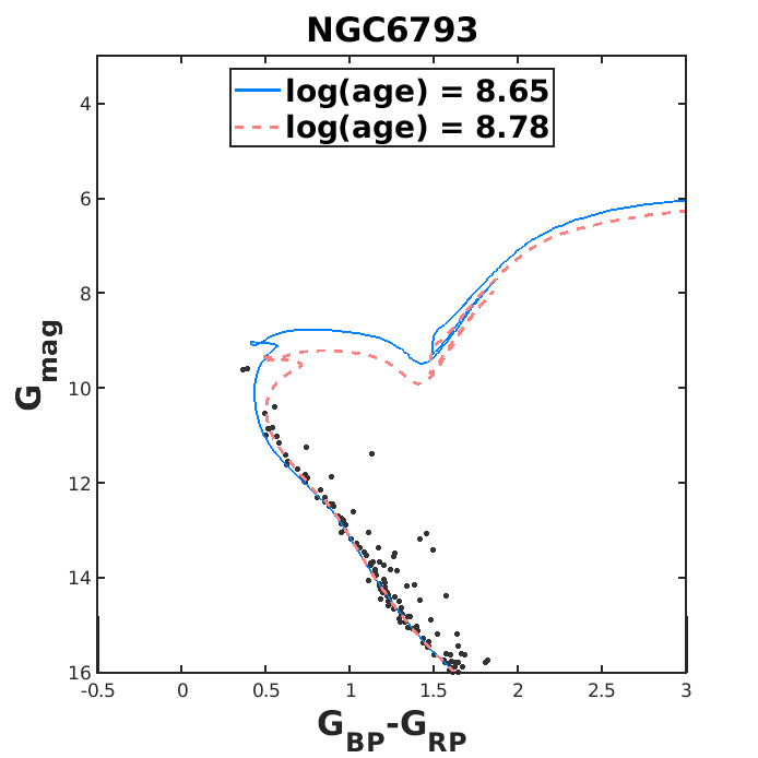 Figure 18
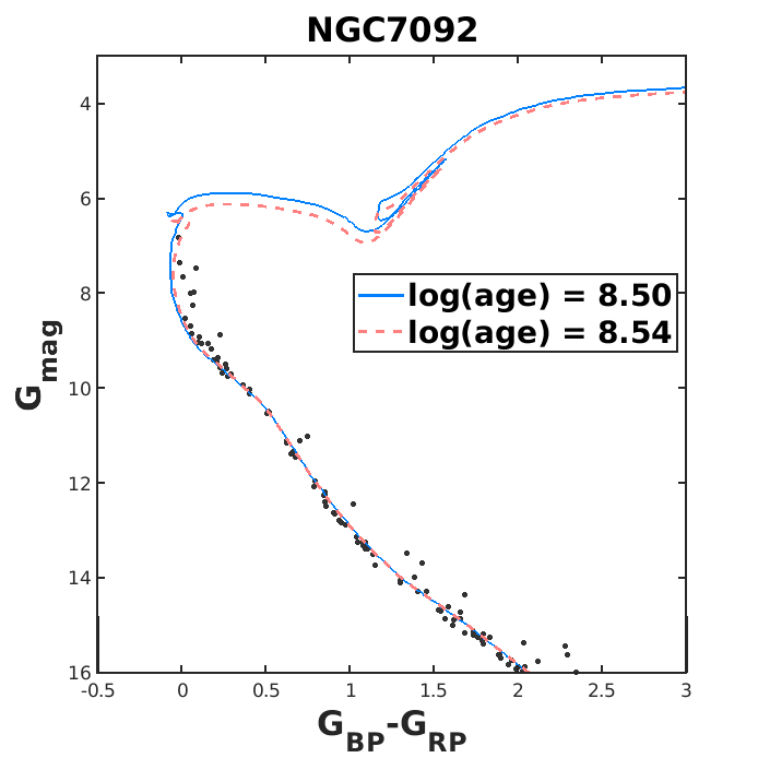 Figure 19
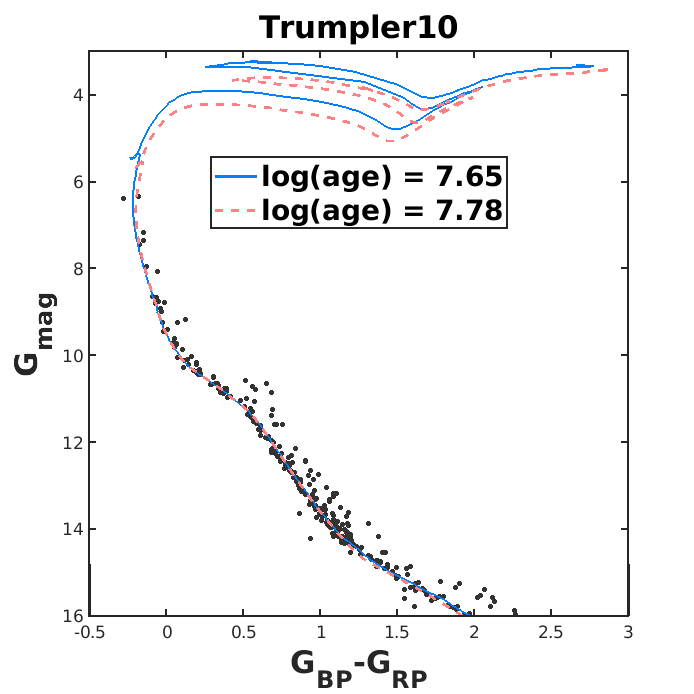 Figure 20
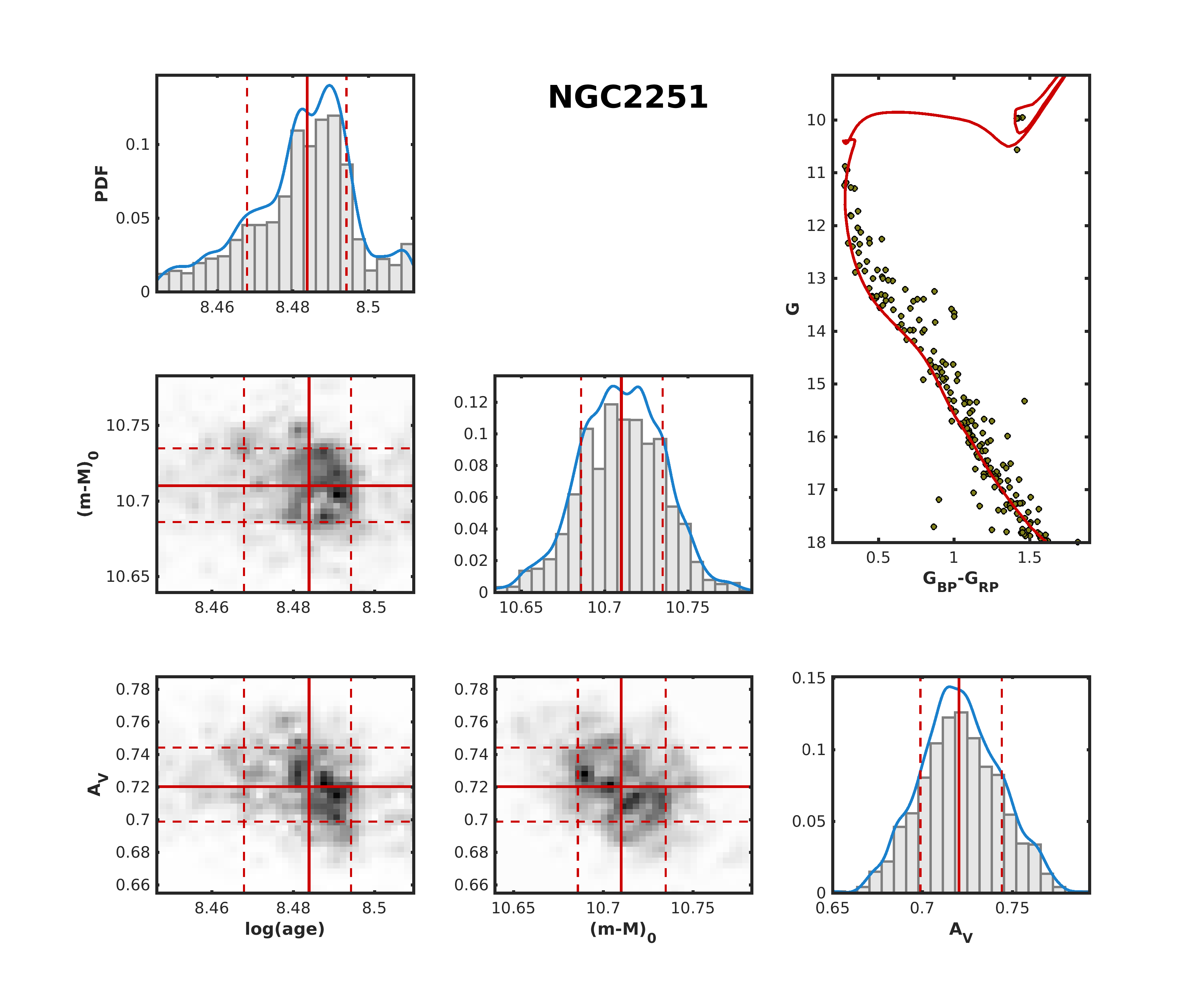 Figure 21
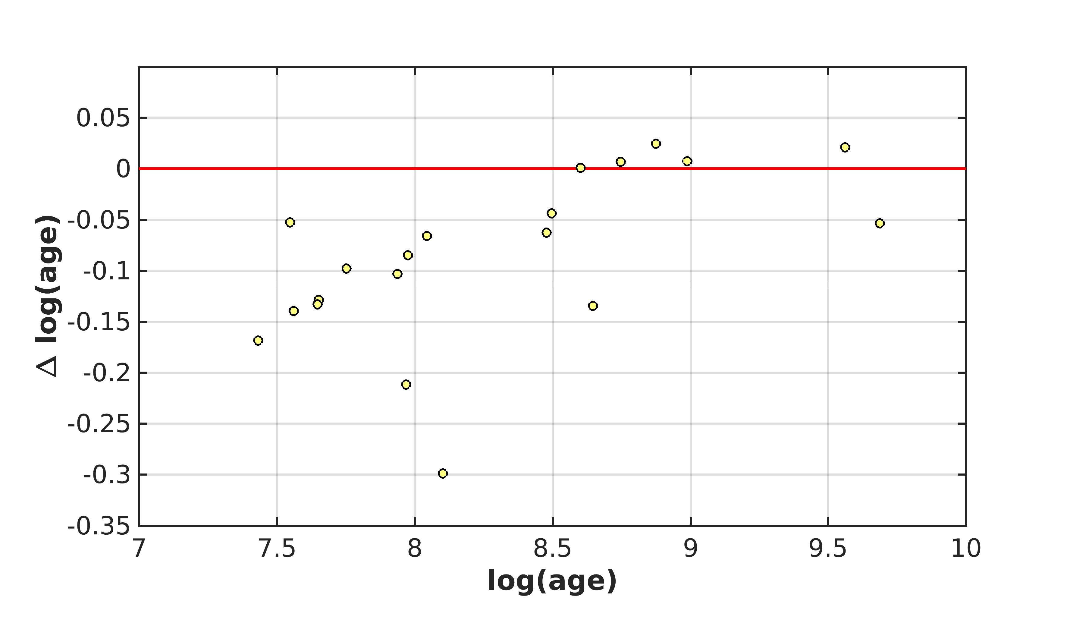 Figure 22
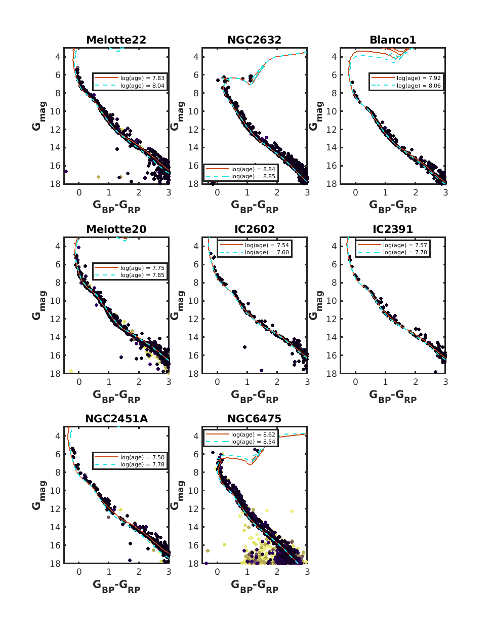 Figure 23
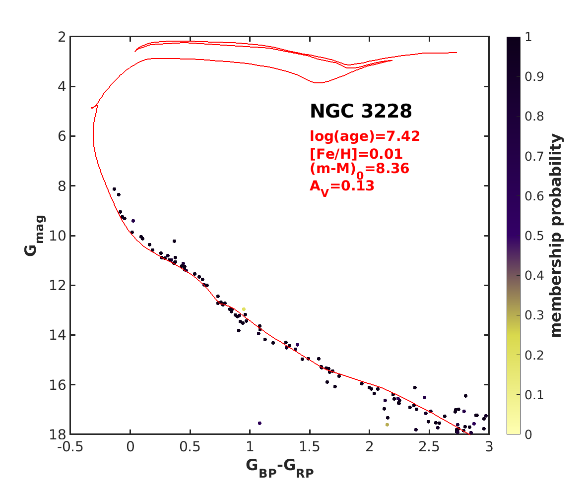 Figure 24
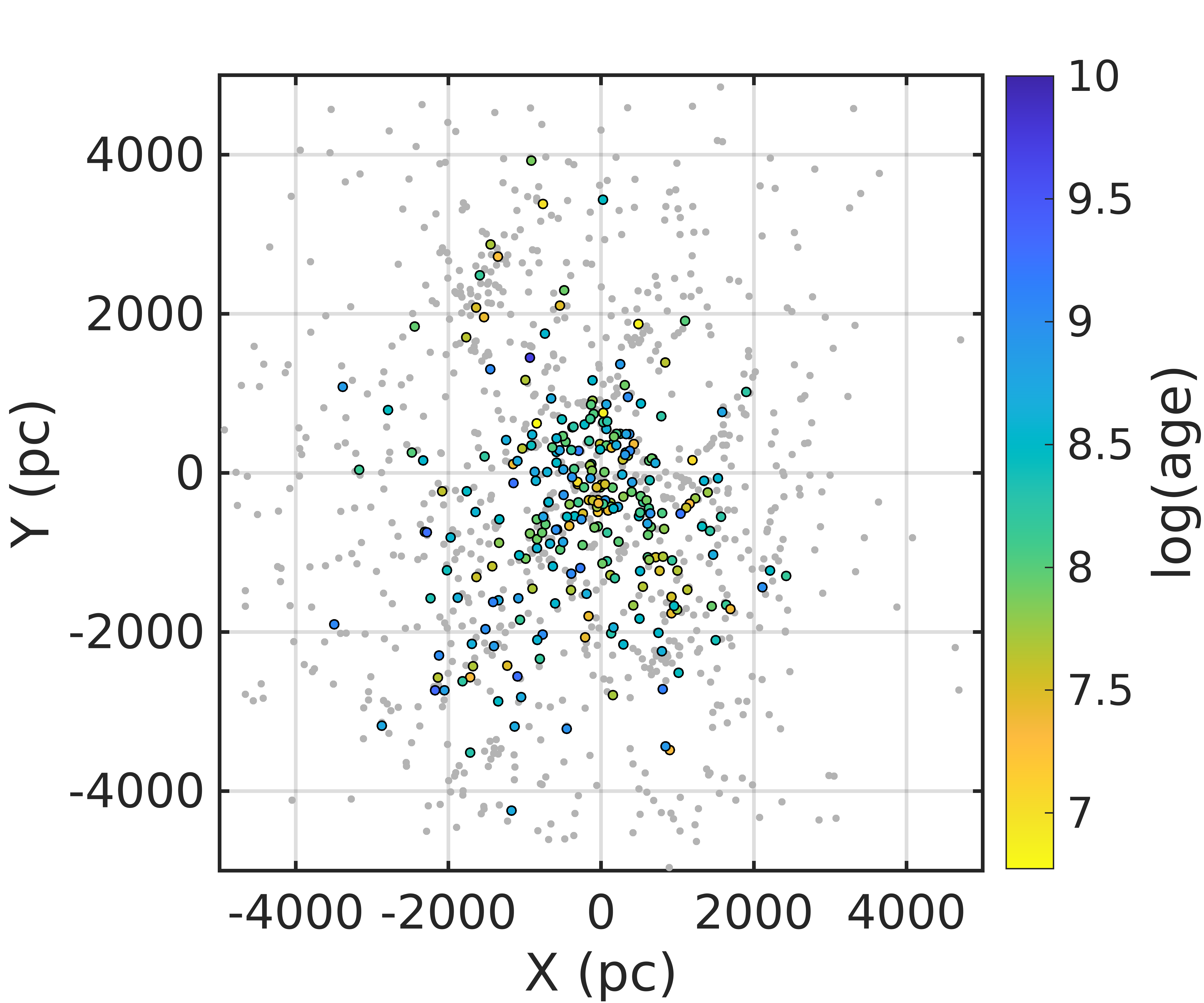 Figure 25
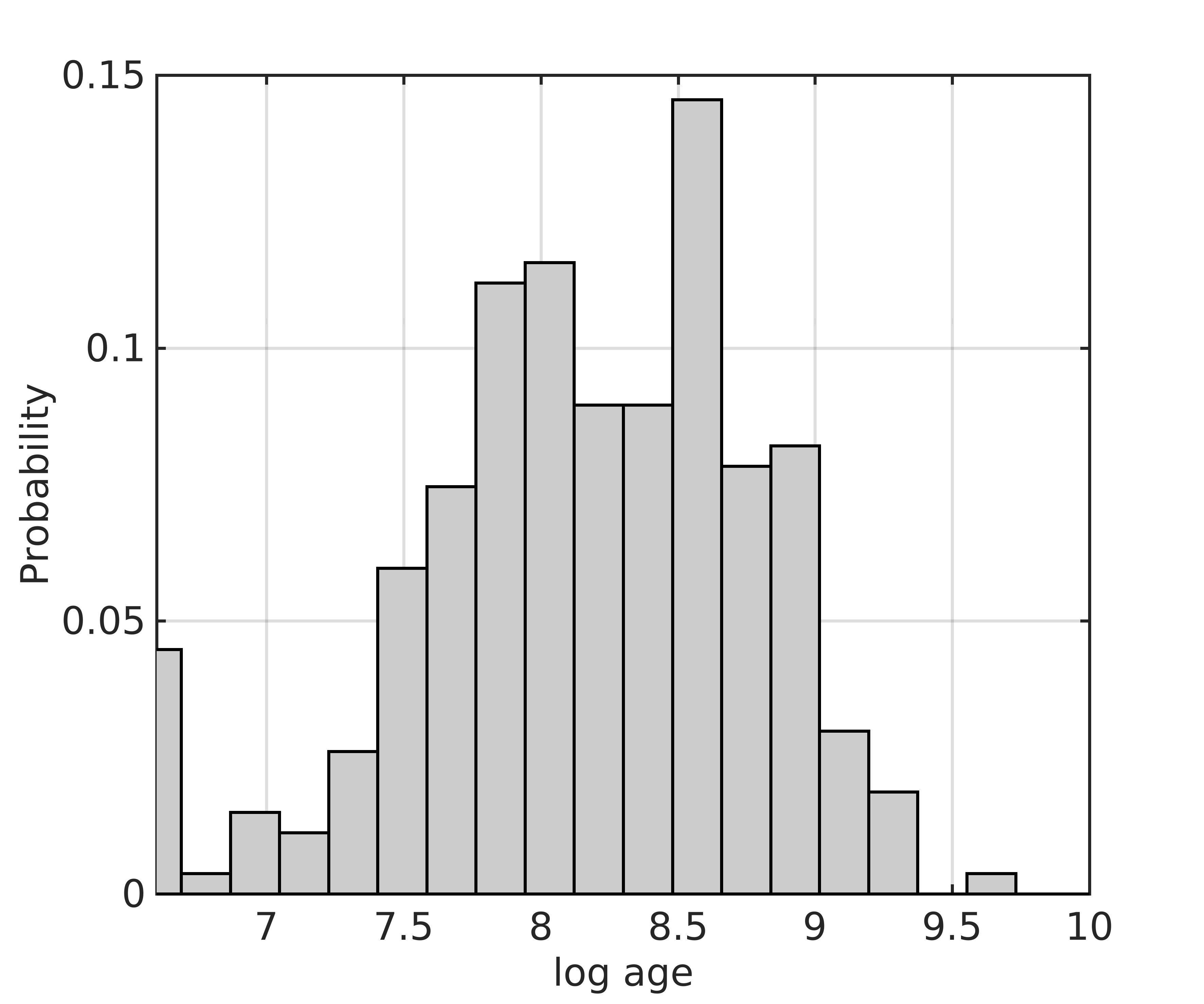 Figure 26
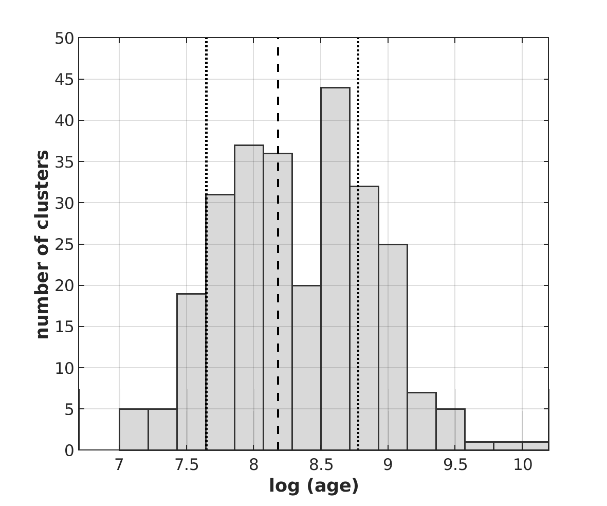 Figure 27
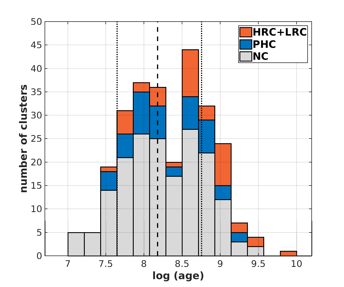 Figure 28
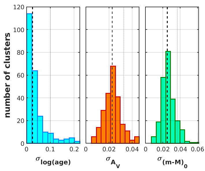 Figure 29
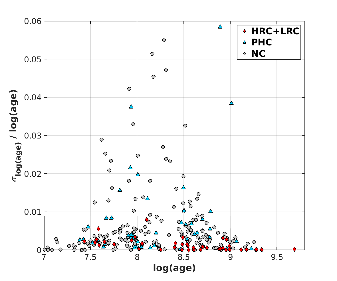 Figure 30
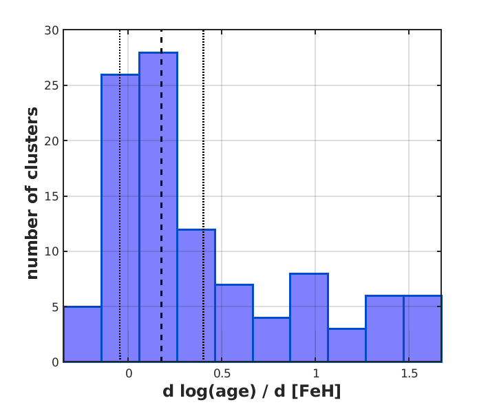 Figure 31
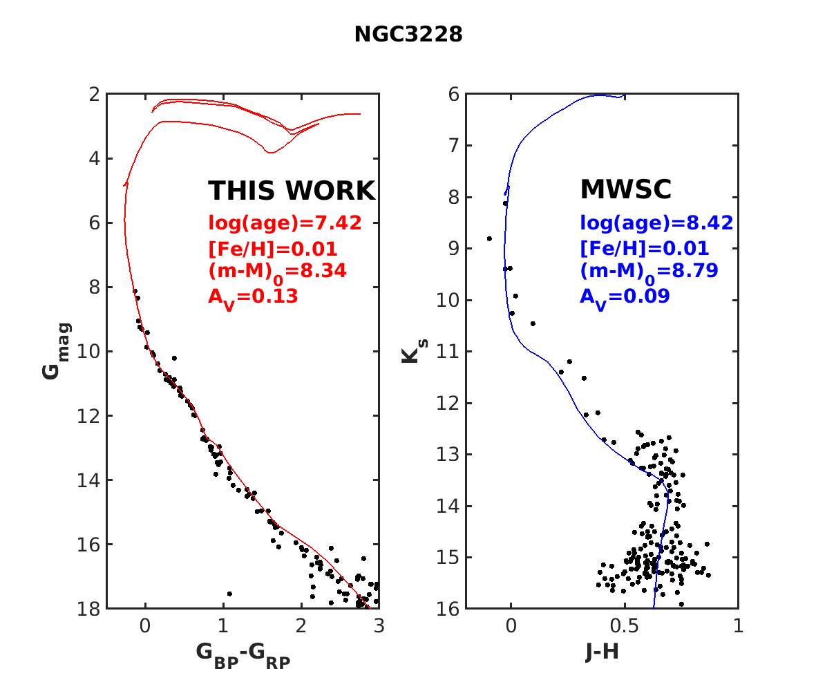 Figure 32
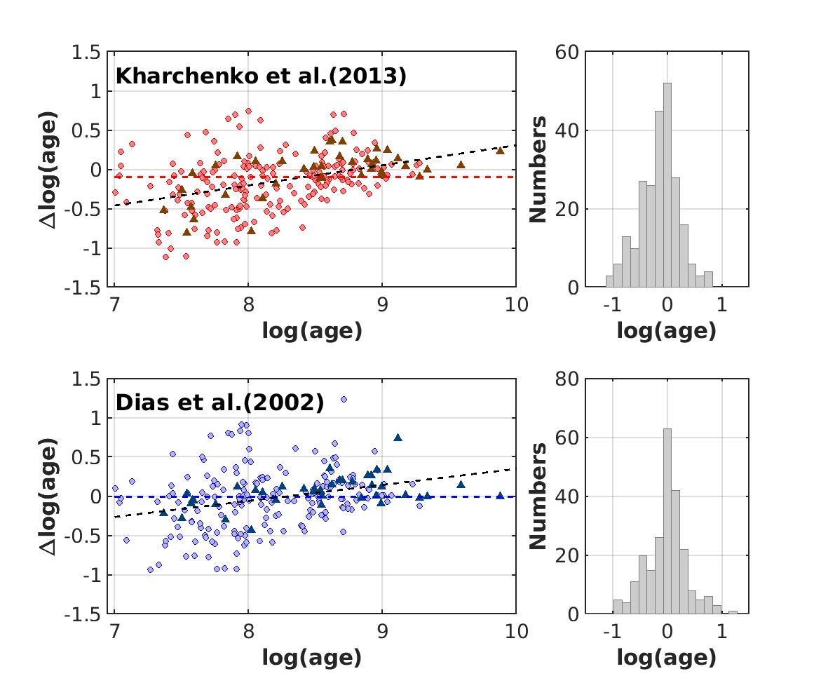 Figure 33
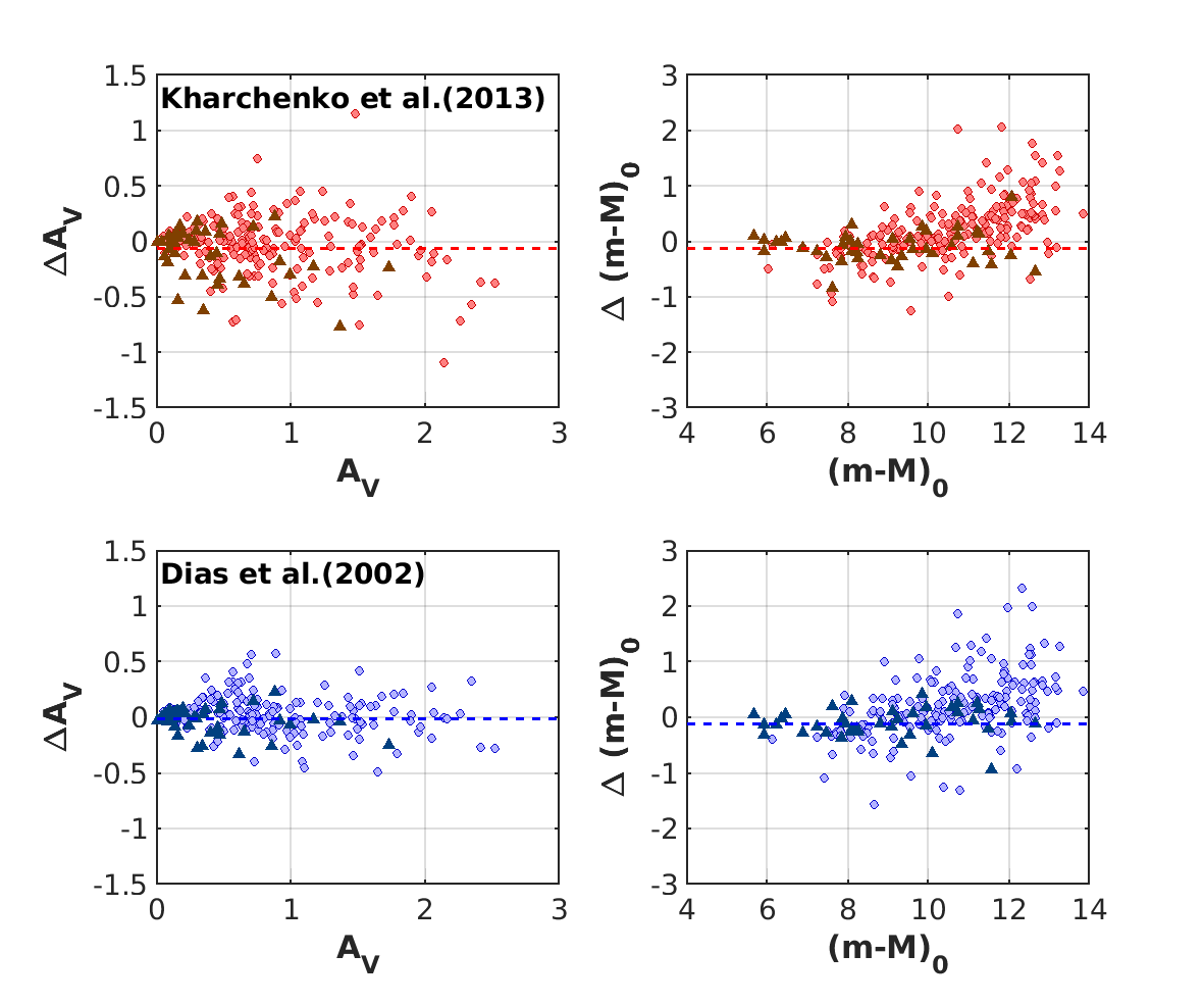 Figure 34
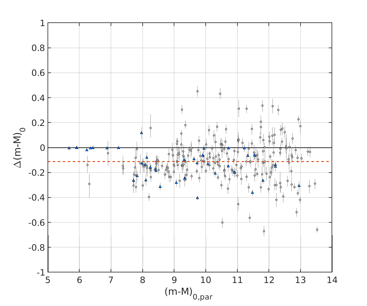 Figure 35
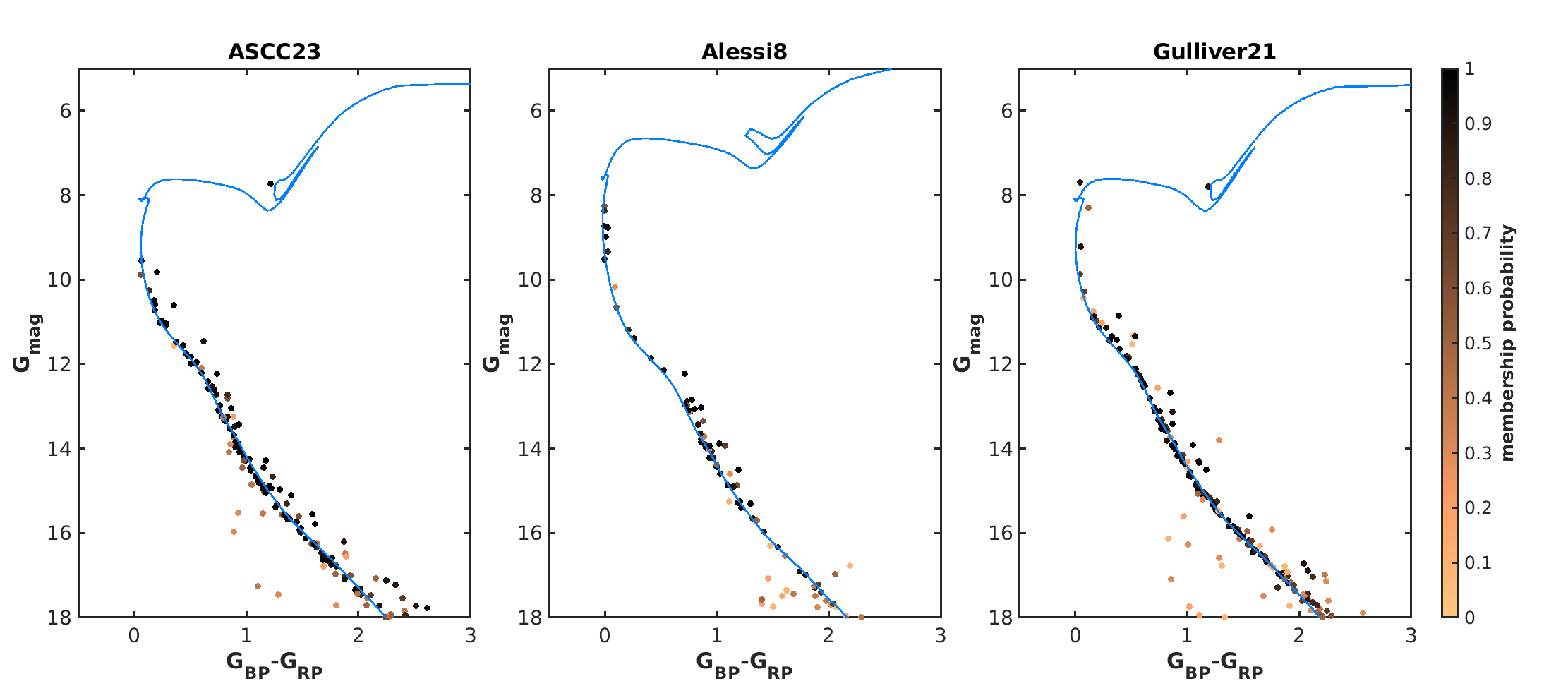 Figure 36
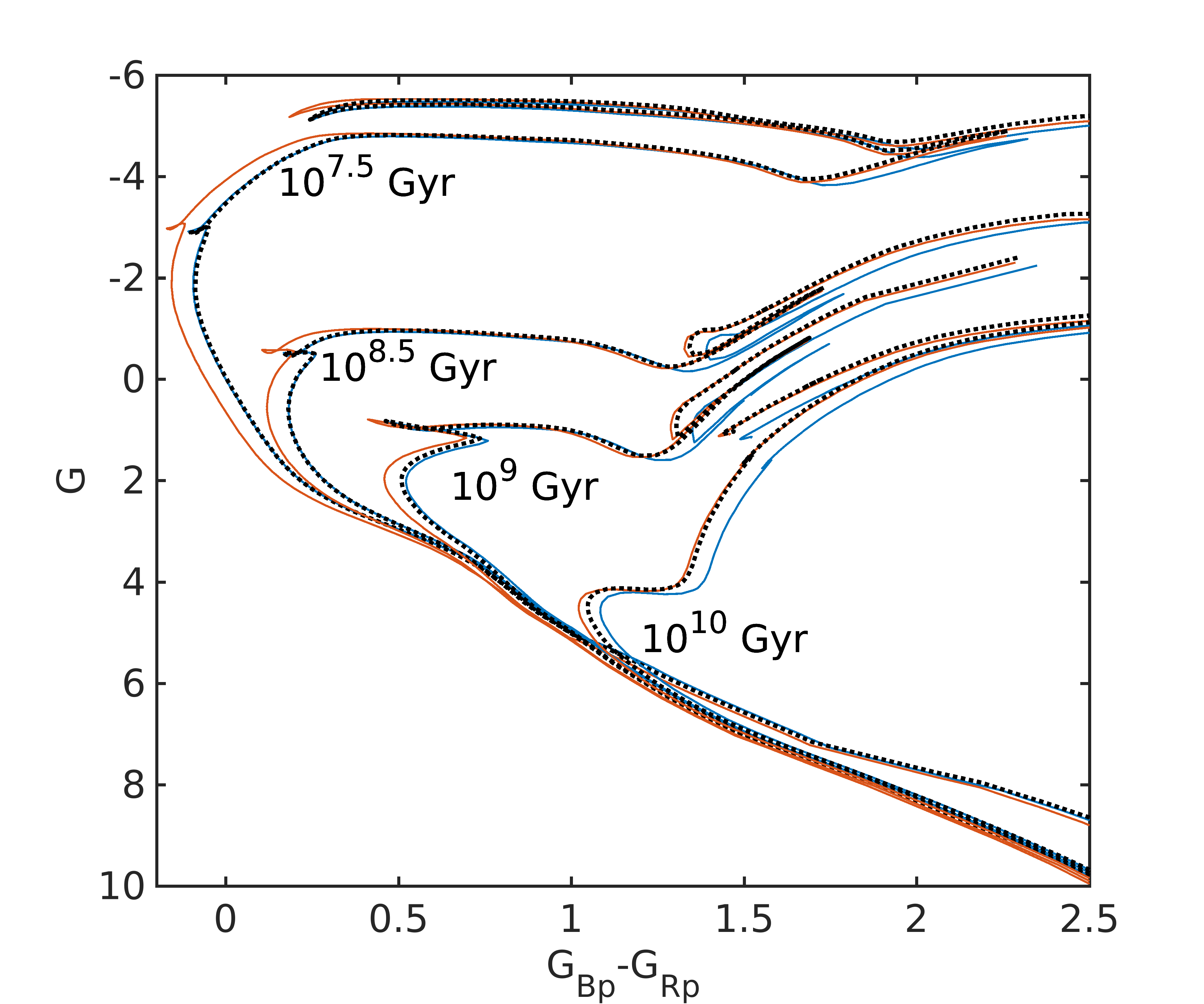 Figure 37
| Gaia Collaboration et al. (2018b) extinction coefficients | |||||||
|---|---|---|---|---|---|---|---|
| median (number of clusters) | ||||
| interval | HRS+LRS | PHC | NC | all |
| 0.0023 ( 6) | 0.0027 ( 8) | 0.0019 ( 41) | 0.0021 ( 55) | |
| 0.0017 (12) | 0.0039 (22) | 0.0047 ( 83) | 0.0040 (117) | |
| 0.0003 (26) | 0.0051 (16) | 0.0034 ( 55) | 0.0027 ( 93) | |
| 0.0007 (44) | 0.0039 (46) | 0.0034 (179) | 0.0029 (269) | |
| Cat. | MADΔlog(age) | MAD | MAD | |||
|---|---|---|---|---|---|---|
| DAML all | 0.00 | 0.17 | -0.01 | 0.07 | -0.11 | 0.29 |
| MWSC all | -0.09 | 0.19 | -0.05 | 0.13 | -0.08 | 0.28 |
| DAML HRS | 0.05 | 0.11 | -0.01 | 0.06 | -0.11 | 0.15 |
| MWSC HRS | 0.04 | 0.10 | -0.06 | 0.14 | -0.11 | 0.15 |
| cluster | ra | dec | [Fe/H] | ||||
|---|---|---|---|---|---|---|---|
| Blanco1 | +0.853 | 0.853 | 7.98 | 6.88 | 0.03 | 0.03 | 0.000 |
| IC2391 | +130.292 | 130.292 | 7.56 | 5.91 | 0.09 | 0.09 | 0.000 |
| IC2602 | +160.613 | 160.613 | 7.55 | 5.91 | 0.10 | 0.09 | 0.000 |
| IC2714 | +169.373 | 169.373 | 8.55 | 10.71 | 0.99 | 0.97 | 0.020 |
| IC4665 | +266.554 | 266.554 | 7.58 | 7.45 | 0.40 | 0.39 | -0.030 |
| IC4756 | +279.649 | 279.649 | 8.99 | 8.40 | 0.40 | 0.39 | 0.000 |
| Melotte20 | +51.617 | 51.617 | 7.75 | 6.21 | 0.28 | 0.27 | 0.140 |
| Melotte22 | +56.601 | 56.601 | 7.94 | 5.67 | 0.14 | 0.14 | 0.000 |
| Melotte71 | +114.383 | 114.383 | 9.11 | 11.55 | 0.48 | 0.47 | -0.270 |
| NGC0188 | +11.798 | 11.798 | 9.69 | 11.49 | 0.26 | 0.26 | 0.000 |
Peer Reviews
No public reviews on file for this paper yet. If you reviewed it on a platform where reviews are public (OpenReview, ICLR, NeurIPS, ICML), you can paste yours below so the community can read it here.
Videos
No videos yet. Explain this paper in a talk, walkthrough, or lecture? Add one.
11institutetext: INAF-Osservatorio Astronomico di Padova, vicolo Osservatorio 5, 35122 Padova, Italy 22institutetext: INAF-Osservatorio di Astrofisica e Scienza dello Spazio, via Gobetti 93/3, 40129 Bologna, Italy 33institutetext: Institut de Ciències del Cosmos, Universitat de Barcelona (IEEC-UB), Martí Franquès 1, E-08028 Barcelona, Spain 44institutetext: SIM, Faculdade de Ciências, Universidade de Lisboa, Ed. C8, Campo Grande, P-1749-016 Lisboa, Portugal 55institutetext: Laboratoire d’Astrophysique de Bordeaux, Univ. Bordeaux, CNRS, B18N, allée Geoffroy Saint-Hilaire, 33615 Pessac, France 66institutetext: Observational Astrophysics, Department of Physics and Astronomy, Uppsala University, Box 516, 75120 Uppsala, Sweden
Age determination for 269 Gaia DR2 Open Clusters
D. Bossini Age determination for 269 Gaia DR2 Open ClustersAge determination for 269 Gaia DR2 Open Clusters
A. Vallenari Age determination for 269 Gaia DR2 Open ClustersAge determination for 269 Gaia DR2 Open Clusters
A. Bragaglia Age determination for 269 Gaia DR2 Open ClustersAge determination for 269 Gaia DR2 Open Clusters
T. Cantat-Gaudin Age determination for 269 Gaia DR2 Open ClustersAge determination for 269 Gaia DR2 Open Clusters
R. Sordo Age determination for 269 Gaia DR2 Open ClustersAge determination for 269 Gaia DR2 Open Clusters
L. Balaguer-Núñez Age determination for 269 Gaia DR2 Open ClustersAge determination for 269 Gaia DR2 Open Clusters
C. Jordi Age determination for 269 Gaia DR2 Open ClustersAge determination for 269 Gaia DR2 Open Clusters
A. Moitinho Age determination for 269 Gaia DR2 Open ClustersAge determination for 269 Gaia DR2 Open Clusters
C. Soubiran Age determination for 269 Gaia DR2 Open ClustersAge determination for 269 Gaia DR2 Open Clusters
L. Casamiquela Age determination for 269 Gaia DR2 Open ClustersAge determination for 269 Gaia DR2 Open Clusters
R. Carrera Age determination for 269 Gaia DR2 Open ClustersAge determination for 269 Gaia DR2 Open Clusters
U. Heiter Age determination for 269 Gaia DR2 Open ClustersAge determination for 269 Gaia DR2 Open Clusters
(Received date / Accepted date )
Abstract
Context. Gaia Second Data Release provides precise astrometry and photometry for more than 1.3 billion sources. This catalog opens a new era concerning the characterization of open clusters and test stellar models, paving the way for a better understanding of the disc properties.
*Aims. *The aim of the paper is to improve the knowledge of cluster parameters, using only the unprecedented quality of the Gaia photometry and astrometry.
*Methods. *We make use of the membership determination based on the precise Gaia astrometry and photometry. We apply an automated Bayesian tool, BASE-9, to fit stellar isochrones on the observed , , magnitudes of the high probability member stars.
*Results. *We derive parameters such as age, distance modulus and extinction for a sample of 269 open clusters, selecting only low reddening objects and discarding very young clusters, for which techniques other than isochrone-fitting are more suitable for estimating ages.
Key Words.:
**Methods: statistical - Galaxy: open clusters and associations - catalogs - Galaxy: stellar content **
1 Introduction
The study of the formation and evolution of Open Clusters (OC) and their stellar populations represents a backbone of research in modern astrophysics. Indeed, they have a strong impact on our understanding of key open issues, from the star formation process, to the assembly and evolution of the Milky Way disc, and galaxies in general (Friel 1995; Jacobson et al. 2016; Cantat-Gaudin et al. 2016; Janes & Adler 1982). With their ages that cover the entire lifespan of the Milky Way thin disc, OCs can be used for tracing the Galactic structure. It is therefore essential to have precise information on a significant number of OCs, located at different Galactocentric distances together with the determination of their parameters (e.g. age, kinematics, distances, and chemistry). In the pre-Gaia era we were still far from an ideal situation: the OC census is in fact poorly known. Currently about 3000 OCs are listed in the most recent versions of Kharchenko et al. (2013, hereafter MWSC) and Dias et al. (2002, hereafter DAML) catalogs. However, the sample is far from being complete even in the local environment (within Kpc, Joshi et al. 2016), where new nearby clusters are still discovered nowadays (see e.g. Cantat-Gaudin et al. 2018a, b; Castro-Ginard et al. 2018). At the faint end of the OC distribution, small and sparse objects and remnants of disrupted clusters can escape detection (Bica & Bonatto 2011). It is also not straightforward to distinguish true clusters from asterisms without high quality kinematic information (Kos et al. 2018). Moreover, studies on OCs may be affected by very large uncertainties on the membership, distance and metallicity and this reflects on the age determination (Netopil et al. 2016; Cantat-Gaudin et al. 2018a).
Gaia has opened a new era in Galactic astronomy and in cluster science, in particular, thanks to the recent second data release (Gaia Collaboration et al. 2018c, a, hereafter GDR2). GDR2 not only provides homogeneous photometric data covering the whole sky, but also unprecedented high precision kinematics and parallax information, that are fundamental to obtain accurate membership and to identify new clusters. This in turn, will allow more precise age determinations.
This paper is part of a series devoted to improve the OCs census and their parameter determination, based on Gaia data. Cantat-Gaudin et al. (2018c) has derived membership probability and parameters for 128 OCs, by combining 2MASS photometry (Skrutskie et al. 2006), Gaia First Data Release (DR1) TGAS parallaxes, and proper motions from either Gaia DR1 or UCAC4 data (Zacharias et al. 2012). Castro-Ginard et al. (2018), Cantat-Gaudin et al. (2018a), and Cantat-Gaudin et al. (2018b) discovered a large number of new OCs using GDR2, and re-classified a significant number of objects that turned out to be likely asterisms and not true clusters. Cantat-Gaudin et al. (2018a, hereafter Paper I) also updated the cluster census in the solar neighborhood, deriving memberships, mean distances and proper motions for 1229 OCs from GDR2. Soubiran et al. (2018) have made use of GDR2 to derive the kinematics of a sample of 861 OCs in the Milky Way, confirming that OCs have a similar velocity distribution to field stars in the solar neighbourhood. This paper aims to carry out automated determination of OC parameters (age, distance, extinction) by isochrone fitting using BASE-9 (von Hippel et al. 2006, see also Jeffery et al. 2016) on Paper I clusters. The final catalog contains bona-fide parameters for 269 clusters. This constitutes an impressive data base to understand not only the formation and evolution of open clusters, but also the disc properties.
Section 2 presents the data and the cluster selection. Section 3 summarizes the method and the priors used to derive OC parameters (i.e. BASE-9). In section 4 we present the ages and the cluster parameters obtained for our sample of OCs. Finally, section 5 compares our results with other surveys.
2 Data: Gaia cluster selection, membership and photometry
We make use of the cluster membership derived in Paper I on the basis of the GDR2 photometry, proper motions and parallaxes. The catalog includes 1229 objects. Paper I has indeed improved the determination of membership for their clusters, thanks to Gaia very precise multi-dimensional astrometric data, with proper motions precision typically of mas yr*-1* (for \mbox{G}=14-18) and parallaxes with precision of mas. We recall that to discard sources with overly large photometric uncertainties, the membership derived in Paper I is limited to sources brighter than \mbox{G}\sim18 (see Evans et al. 2018, for details). ite This corresponds to the turnoff of a 3 Gyr cluster seen at 10 Kpc, assuming no interstellar extinction. The more distant and older OCs are therefore out of our detection threshold. We restrict our analysis to a selection of OCs, having low extinction ( mag) and ages older than 10 Myr (according to MWSC and DAML catalogs). For younger clusters, where the unclear identification of the main-sequence turnoff (TO), contamination of Pre-MS stars, and possible age spread can compromise the isochrone-fitting method, other independent techniques are more suitable to estimate the age (see, e.g., Bouvier et al. 2018; Jeffries et al. 2017; Jeffries 2017; David & Hillenbrand 2015). The final sample counts 269 OCs, located within Kpc. Clearly, due to the selection criteria we applied, our sample is far from being complete.
In this work we make use only of the photometry from GDR2 in its three bands , , and . This is motivated by the exceptional quality of this photometry, having a precision of the order of a few millimag (see for instance Gaia Collaboration et al. 2018b). Figure 1 presents color-magnitude diagrams (CMD) of a few poorly studied clusters, namely ASCC 23, Alessi 8, and Gulliver 21. In all these objects, the main sequence and the equal mass binary sequence can be clearly identified.
3 Method: Bayesian parameter determination
Handling the large, three-dimensional GDR2 datasets requires automated methods in order to characterize the OCs. To determine the parameters of our sample we use an open-source software suite known as BASE-9 (von Hippel et al. 2006), that introduces a Bayesian approach to compare observational distribution of magnitudes of stellar members of a cluster in different bands with a set of theoretical isochrones. The Bayesian method requires a likelihood function, i.e. the distribution of the data given the model parameters. The knowledge about the model parameters before considering the current data defines the prior distribution, while the combined information in the data and our prior knowledge give the posterior distribution.
BASE-9 can adjust four parameters (age, metallicity, absorption, and distance modulus) at each iteration, using a Monte Carlo-Markov chain algorithm (MCMC). BASE-9 provides estimate of the posterior probability distribution (PDF) for a given number of iterations. Each iteration point is linked to the next by a “random walk” process described in von Hippel et al. (2006) van Dyk et al. (2009), to which we also refer for a deeper description of BASE-9. The introduction of priors is very useful to avoid or at least reduce local minima. Our choice of priors is described in the section 3.3. Visual inspection of the trace plot (parameter value against iteration number) shows that all the iteration chains reach their apparent stationary distributions within the first 1000 steps. This tuning period (called burn-in phase) is then discarded from the subsequent analysis. Each chain continues for an other 10,000 iterations in order to ensure statistical relevance of the results. The clear advantage of this automated Bayesian approach for model fitting is to provide principled and reproducible estimates and uncertainties on all parameter.
The following paragraphs describe the main set-up and inputs we used in our BASE-9 computation.
3.1 Stellar models and isochrones
By default, BASE-9 comes with a large library of isochrones computed by different stellar-evolution groups. However none of this set of models include photometry in Gaia DR2 passbands (Evans et al. 2018, revised version). Therefore we replaced the BASE-9-implemented PARSEC set (Bressan et al. 2012) with an updated version where also GDR2 passbands are available111http://stev.oapd.inaf.it/cgi-bin/cmd. Our grid consists of isochrones in the range of 222logarithm of age given in years. between 6.60 and 10.13 with a step of 0.01, and [Fe/H] between -2.10 and +0.50 with a step of 0.05. For this work we use the release PARSEC v1.2S with the bolometric corrections described by Chen et al. (2014). These authors implement the relation between the temperature T and Rosseland mean optical depth across the atmosphere from PHOENIX BT-Settl models as the outer boundary conditions for low temperatures. In addition the PARSEC isochrones include a re-calibration of the mass-radius relation for cool dwarfs as derived from eclipsing binaries. This isochrone set has been proven to reproduce not only the lower main sequence, but also all the CMD features in more than 30 nearby OCs in GDR2 (see Gaia Collaboration et al. 2018b).
3.2 Interstellar extinction
In BASE-9 the absorption is described using the parameter , which is the extinction in the band. However, using different set of bands (i.e. the Gaia bands), it is necessary to translate into a proper measure of the extinction in the specific bands. Due to the large width of the Gaia bands, the coefficients , where can be , , and , are dependent from the stellar effective temperature (Jordi et al. 2010; Danielski et al. 2018; Gaia Collaboration et al. 2018b). Therefore, we can expect a deviation in the shape of the reddened isochrone if a fixed relation is adopted. A more sophisticated approach was introduced in Danielski et al. (2018) and implemented in Gaia Collaboration et al. (2018b). In this case the extinction coefficients of the Gaia bands were defined as functions of the absorption itself and the stellar effective temperature, in the term of the color :
[TABLE]
where belong to a set of coefficients defined in Gaia Collaboration et al. (2018b) for , , and . The terms represents also the fixed extinction coefficients calibrated for a A0V star. All the coefficients are listed in Table 1. The results presented in Tables A, A and A are given in terms of , the extinction in at the turnoff of the cluster, and , the extinction parameter to be used in equation 1 to derive the dependence on color (and therefore temperature).
3.3 Choice of Priors
The Bayesian approach has the advantage that previous independent results can be incorporated through the joint prior distribution, that can be specified via independent priors on each parameter. BASE-9 needs priors on the age, metallicity ([Fe/H]), , and on the distance modulus. To set those values we refer to literature where possible. Concerning extinction, we use the values from DAML or MWSC catalogs (prioritizing the first), where available, otherwise we set prior to 0.1 mag, respectively. has been marginalized within a (or 0.033 mags if ). No restriction is instead applied on the age and the variable is left free to vary inside the whole isochrone grid. The prior on the distance modulus is estimated through parallax inversion, which is equivalent to the equation:
[TABLE]
where is the intrinsic distance modulus and is the median value of the parallax of the cluster members. As discussed by Luri et al. (2018), such determination of distance is a very poor approximation, since systematics and correlations in the Gaia astrometric solution tend to overestimate the true distance, that should instead be obtained by Bayesian inferences (see, e.g., Bailer-Jones et al. 2018). Eq. 2 gives more consistent results for very close objects, having uncertainties on the parallax lower than 5-6% (see Gaia Collaboration et al. 2018a, b) This justifies our assumption that for clusters closer than 1 Kpc and having almost no extinction, the distance modulus is assumed to be fixed to the value of equation 2. This is the case for the clusters in common with Gaia Collaboration et al. (2018b) table 2 (see also Sect. 5). In all the other cases, the distance modulus is derived from the posterior distribution of the BASE-9 solutions, as recommended by Luri et al. (2018). We must stress that BASE-9 looks for the observed modulus, and therefore we set the prior to include the contributions of both distance and extinction:
[TABLE]
Finally we choose to keep [Fe/H] fixed during the BASE-9 runs, in order to reduce the degeneracy within the variables. We divide our sample in three categories having different uncertainties on the [Fe/H] determination: (1) clusters with high (HRS) and low resolution spectroscopy (LRS) determination of metallicity, (2) clusters with other determination of metallicity (photometric determination, PHC), and (3) clusters with no information on metallicity (NC). High resolution metallicity determinations include data from Netopil et al. (2016) and Gaia-ESO (Spina et al. 2017; Magrini et al. 2017). Concerning LRS and PHC clusters, we make use of the compilations by Heiter et al. (2014) (using spectroscopy), Paunzen et al. (2010) (using photometry) as homogenized and re-calibrated by Netopil et al. (2016), who bring them on a common scale, producing the he largest homogeneous compilation of OC metallicities by far. To this group we add a few clusters whose metallicity information is taken from DAML. When this is not available we use the MWSC catalog. If no other information is found in the literature (NC clusters), we set [Fe/H]=0.0. This is a reasonable assumption, looking at the metallicity of the OCs that are in the range (Netopil et al. 2016). The number of clusters in each group is reported in Table 2. Since using different sources for [Fe/H] can introduce several biases, we discuss the implication of all the above priors on the OC parameter determination in section 4.1.2.
3.4 Post-process analysis
The probability distribution of the posteriors in BASE-9 are calculated during the post-process analysis. For each run, once the chain converges, the iterations are generally distributed around a single high-probability solution. We estimate this solution through the medians for the three variables (i.e. age, extinction, and distance modulus), neglecting low probability solutions when present. Runs having multiple (very different) solutions of comparable probability are regarded as unreliable and discarded.
It is important to notice that in principle Red Giant Branch and Red Clump stars could be used to set constrains on the metallicity. In fact, the locations of these phases on the CMD are sensitive to the change of [Fe/H]. However the majority of our clusters, with a few exceptions, show CMDs without these features or with only a few Red Giant stars (RG), therefore the fit is largely dominated by main sequence stars. As a final note, we point out that each result has been checked visually, discarding clusters with a poor isochrone fit.
4 Results
The final sample of OCs span a range of 7.0$$<\log(age)<$$10.0. Fig. 2 shows an example of the output for NGC 2251. On the three diagonal panels we show the probability distribution function of the variables with their median values (red solid line), while in the top-right panel we present the CMD of the cluster where the isochrone corresponding to the median values of the solutions is overplotted.
The parameter determination for the three groups of clusters including the priors on [Fe/H] are listed in Table A (44 OCs), Table A (46 OCs), and finally Table A (179 OCs) for HRS+LRS, PHC, NC objects, respectively. The values are referred to the median of each posterior distribution, while the uncertainties correspond to the 16th and 84th percentiles. Fig. 3 presents the age distribution of the studied clusters.
4.1 Estimate of Uncertainties
In the following paragraphs we estimate the random errors on the solutions and the systematics resulting from our assumptions on [Fe/H].
4.1.1 BASE-9 internal uncertainties
Estimation of parameter uncertainties has been done by considering the and percentiles (corresponding to ) of the iterations distribution for each posterior (see Fig. 2). The distribution of the internal uncertainties for all the parameters is given in Fig. 4.
We find that 90% of the clusters have sigmas smaller than, respectively, , , and , while their medians are , , and . While the extinction and the distance modulus determination are well confined, the distribution of the uncertainties on the presents a tail of about 30 OCs having . Typical examples of this category of objects are Gulliver 20, IC 2157, and Ruprecht 29. These clusters are characterized by having no information on [Fe/H] (i.e we assume [Fe/H]=0.0); high extinction () and a low number of members. For these reasons, their fits are not well constrained, and the solutions present a high degree of degeneracy between the extinction and the distance modulus. Fig. 5 and Table 3 shows the distribution of the relative error on . HRS and LRS clusters have smaller internal uncertainties, while clusters belonging to the PHC group present larger errors. We detect no trend of as a function of the .
4.1.2 Impact of fixed-metallicity prior
As discussed in Sect.3.3, we use a fixed metallicity in our BASE-9 calculations, and this can have an impact on results. The aim of this section is to estimate the degree of degeneracy between the parameter determination and [Fe/H].
We select from our catalog a sample of 100 clusters spanning the whole age range we consider, and we run BASE-9 on them using three different priors on the metallicity, . In this test, the metallicity is let free to vary within a . Using these three runs, we calculate for the three solutions of each cluster the regression line on the plane . The slope gives the predicted variation of the within 1 dex in metallicity for that specific cluster. Considering the overall distribution, we find a median slope of 0.18 with a median absolute deviation (MAD) of 0.22 (see Fig. 6). Clearly the systematics we introduce on the OC parameter determination are different depending on the uncertainties on the [Fe/H] priors (see Table 2). The effect can be negligible in the case of objects having [Fe/H] determination from high resolution spectroscopy. Assuming as typical the sigma of 0.06 dex on [Fe/H] determination as derived from high resolution spectroscopy in the Gaia ESO public survey (see for instance Jacobson et al. 2016), we obtain
[TABLE]
As we mentioned, for the NC group we assume [Fe/H]=0.0. Looking at the distribution of the metallicity of Galactic clusters, we expect that all objects are inside a . In this case we estimate an effect on of , which, translated in linear age, corresponds to about . Clusters having [Fe/H] from photometry or low resolution spectroscopy can be regarded as having intermediate uncertainties. In the case of PHC objects, we find a median value of , resulting in , while for the LRS sample we derive , corresponding to .
The apparent distance modulus variations at changing [Fe/H] are quite small, with a median value for the extreme case when we assume [Fe/H]=0.0. However, the extinction and the absolute distance modulus solutions are more affected by the assumption on [Fe/H], with a clear degeneracy. We find a median value of and for the extinction and the absolute distance modulus respectively.
5 Discussion
5.1 Comparison with benchmark clusters
We compare our results with a set of well studied clusters having high quality determination of the parameters.
5.1.1 Nearby OCs
In our sample we have 20 nearby clusters already studied by the Gaia Collaboration et al. (2018b) using GDR2 data. In Fig. 7 we compare the age determination in both papers. Both determinations agree within a few percent, showing however a small systematic underestimate for the younger objects. This deviation is mainly due to the fact that the majority of the clusters are inconspicuous (see Fig. 8). In some cases differences between the two ages can be ascribed to the membership determination. One example can be NGC 6793 (see Fig. 8). In this very poorly studied cluster, the bright star at \mbox{G}\sim 9 has a high probability membership from Paper I, while in the Gaia Collaboration et al. (2018b) it is not considered as a member: this changes the position of the MSTO and, therefore, the age from to . We find a similar trend also when comparing with MWSC and DAML (see Section 5.2).
5.1.2 Comparison with asterosesimic data
Our sample contains also three OCs studied by Kepler (Borucki et al. 2010), i.e. NGC 6791, NGC 6811, and NGC 6819. In many of their red-giant stars, solar-like oscillations have been detected, providing global seismic parameters such as the large separation and the frequency of maximum oscillation power . These quantities, combined with the effective temperature, can be used to derive stellar masses through the so-call scaling relations (see, e.g., Kallinger et al. 2010 and Mosser et al. 2010).
In turn, the mass can be used to provide an indirect validation of our age determination. We compare previous estimations of RG masses for these clusters with the range of values corresponding to the same evolutionary phases along our isochrones.
NGC 6791
Seismic determination of the average RGB mass for NGC 6791 gives a value of M*⊙* (Miglio et al. 2012, considering stars up to the RC luminosity). However, it was demonstrate that scaling relations tend to overestimate the value of the mass of RGB stars (White et al. 2011, Brogaard et al. 2018 and reference therein), therefore an additional calibration is required (Rodrigues et al. 2017). This introduces a systematic on the mass of M*⊙*. The estimation of the mass from RGB eclipsing binaries is , in agreement with the previous seismic determination (Brogaard et al. 2012).
Both the measures are perfectly compatible with the mass of M*⊙*, as derived averaging the masses from the bottom of the RGB up to the RC luminosity for an isochrone of the age of , corresponding to our solution.
NGC 6811
Sandquist et al. (2016) determined the masses for 6 stars, 5 of them belonging to the red-clump phase, plus 1 RC candidate. The average value is M*⊙, which is compatible with our average mass determination of M⊙* for the red-clump phase in an isochrone of .
NGC 6819
Handberg et al. (2017) derived seismic parameters for 54 RG stars in NGC 6819. Within the sample, they were able to distinguish between RGB and RC stars. They also identified non-member stars (3), stars classified as overmassive (6), uncertain cases (5), and 1 Li-rich RC. In a subsequent work, Rodrigues et al. (2017) estimated individual masses and ages for 52 RC stars. They compared observational data, including seismic constrains from Handberg et al. (2017), with a grid of models through a Bayesian method (PARAM, da Silva et al. 2006). Using only single RGBs they found an average mass of M*⊙*. Our BASE-9 solution for NGC 6819 corresponds to an isochrone of , that gives an average mass for the RGB of . This values shows only a partial compatibility with Rodrigues et al. (2017) determination, lying within , since they find an age of using a different set of stellar models by Bossini et al. (2015).
5.2 Comparison with MWSC and DAML catalogs
We have 242 clusters in common with MWSC and 234 with DAML. Fig. 9, Fig. 10 and Table 4 show the difference among our determination of age, extinction, and distance for those clusters included in these catalogs.
The median value of the age distribution is mainly consistent with DAML catalog, and shows a systematic of with MWSC. The dispersion is very large in both cases, especially for young clusters, but it is smaller for objects belonging to the HRS group. In addition a clear trend of the age difference with age is present, in the sense that results from BASE-9 are generally younger for OCs below . These deviations are not surprising and might be ascribed to the quality of the cluster membership determination. Previous membership determinations are based on ground based photometry and/or proper motions and are severely hampered by field star contamination. This problem is particularly age-related. In fact, while old clusters can count on better populated features (MS, RGB, and RC) that help the age determination from isochrone fitting, in young clusters the fit is generally based on the luminosity of the MSTO, which may be not well defined, due to the lack in the number of bright near-TO stars. In such a scenario, a different determination of membership, with the addition of bright TO stars, can change the estimation of the age (as we already saw in Sect. 5.1.1 for NGC 6793).
Fig. 10 compares globally our estimates of and with the MWSC and DAML. Globally, no systematic, or a very small one, is present between this work and the literature concerning the value of , but with a large dispersion. The distance modulus exhibits a median difference for both catalogs, getting worse at , where it becomes for MWSC and DAML catalogs respectively.
Fig. 11 shows the difference between the distance moduli derived from the analysis of BASE-9 results (, i.e. the posteriors) and from the inversion of the median parallax (, see Eq.2). We derive a median offset of (. As already discussed in previous sections, the inverse of the parallax tends to overestimate the distance modulus. This is specially true when the relative uncertainty on the parallax is higher than 20%, but it holds also when the uncertainties are lower than that. Here the majority of the clusters are more distant than 1 Kpc, in a regime where the uncertainties on the single star parallaxes are higher than 20%. Averaging the uncertainties on the number of stars in a cluster does not reduce systematics and correlations. The offset we find corresponds to a medium offset of +0.021 mas in parallax. This value is in good agreement with the well-known systematic found in Gaia parallaxes and reported in Gaia Collaboration et al. (2018d).
In addition, the results show a large dispersion, with differences up to mag. We cannot exclude that this due to some other effects, such as uncertainties on the extinction coefficients, or on the assumptions on the metal content. Stochastic effects on the Color-Magnitude diagrams of the less populated clusters can also play a significant role, as well as effects related to stellar evolution (rotation, convection) and binarity.
6 Conclusions
In this work we make use of an automated method based on Bayesian classification, BASE-9, to derive the age of 269 OCs using GRD2 photometry. The parameter determination precision is , , and , while, their medians are , , and . In all the calculations we assume a fixed value of the metallicity [Fe/H], taking it either from high or low resolution spectroscopy or from photometry. When no information is available, we assume . We discuss the effect that the prior has on our results through a series of numerical sensitivity experiments. We find that in the worst case (no information on [Fe/H]), we have a . Comparing our results with existing literature data, we find a large dispersion on age, and with no or a little systematics. On average younger ages are affected by large differences with existing catalogs. This could well be due to the high quality of the Gaia data, i.e. more reliable membership determination and photometry. However, we cannot exclude that BASE-9 tends to underestimate the ages of young clusters. We point out that this is the largest data base of OC parameters derived using homogeneous and high quality data and this method. In this work we make use only of the information from the three Gaia bands. This is motivated by the high quality of the Gaia photometry. However, BASE-9 runs show that using only these magnitudes is not possible to resolve the degeneracy between the four cluster parameters, mainly the distance modulus and the extinction (see also Andrae et al. 2018). For this reason we have analyzed only low extinction objects. A further development will be to use information from complementary photometry to alleviate the degeneracy and extend the present catalog to higher extinction regimes.
Acknowledgements
This work makes use of data products from: the ESA Gaia mission (gea.esac.esa.int/archive/), funded by national institutions participating in the Gaia Multilateral Agreement. This work was supported by ASI (Italian Space Agency) under contract 2014-025-R.1.2015. AB acknowledges funding from PREMIALE 2015 MITiC. This work was supported by the MINECO (Spanish Ministry of Economy) through grant ESP2016-80079-C2-1-R (MINECO/FEDER, UE) and MDM-2014-0369 of ICCUB (Unidad de Excelencia ’María de Maeztu’). C.S. and L.C. acknowledge support from the CNES and from the ”programme national cosmologie et galaxies” (PNCG) of CNRS/INSU. The Portuguese Fundação para a Ciência e a Tecnologia (FCT) through the Strategic Programme UID/FIS/00099/2013 for CENTRA” UH acknowledges support from the Swedish National Space Agency (SNSA/Rymdstyrelsen).
Appendix A CLUSTER TABLES
The reference list from the paper itself. Each links out to its DOI / PubMed record.
- 1Andrae et al. (2018) Andrae, R., Fouesneau, M., Creevey, O., et al. 2018, A&A, 616, A 8
- 2Bailer-Jones et al. (2018) Bailer-Jones, C. A. L., Rybizki, J., Fouesneau, M., Mantelet, G., & Andrae, R. 2018, AJ, 156, 58
- 3Bica & Bonatto (2011) Bica, E. & Bonatto, C. 2011, A&A, 530, A 32
- 4Borucki et al. (2010) Borucki, W. J., Koch, D., Basri, G., & et al. 2010, Science, 327, 977
- 5Bossini et al. (2015) Bossini, D., Miglio, A., Salaris, M., et al. 2015, MNRAS, 453, 2290
- 6Bouvier et al. (2018) Bouvier, J., Barrado, D., Moraux, E., et al. 2018, A&A, 613, A 63
- 7Bressan et al. (2012) Bressan, A., Marigo, P., Girardi, L., et al. 2012, MNRAS, 427, 127
- 8Brogaard et al. (2018) Brogaard, K., Hansen, C. J., Miglio, A., et al. 2018, MNRAS, 476, 3729