On the Bimodal Spin Period Distribution of Be/X-ray Pulsars
Xiao-Tian Xu (NJU), Xiang-Dong Li (NJU)

TL;DR
This paper explains the bimodal distribution of Be/X-ray pulsar spin periods by modeling their spin evolution with a magnetically threaded accretion disk, accounting for transient accretion and disk changes.
Contribution
It introduces a comprehensive model including transient accretion and disk structure changes to explain the bimodal spin period distribution.
Findings
Current pulsars are near spin equilibrium.
Bimodal distribution is reproduced by equilibrium spin periods.
Model aligns with observed period peaks.
Abstract
It has been reported that there are two populations of Be/X-ray pulsars, with the pulse period distribution peaked at 10 s and 200 s, respectively. A possible explanation of this bimodal distribution is related to different accretion modes in Be/X-ray binaries. In this work, we investigate the spin evolution of Be/X-ray pulsars based on the magnetically threaded accretion disk model. Compared with previous works, we take into account several distinct and important factors of Be/X-ray binaries, including the transient accretion behavior and possible change of the accretion disk structure during quiescence. We demonstrate that current Be/X-ray pulsars are close to the spin equilibrium determined by the balance of spin-up during outbursts and spin-down during quiescence, and that the observed bimodal distribution can be well reproduced by the equilibrium spin periods with…
Click any figure to enlarge with its caption.
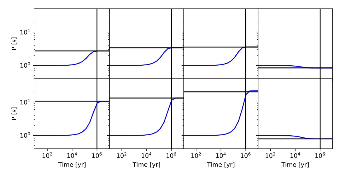 Figure 1
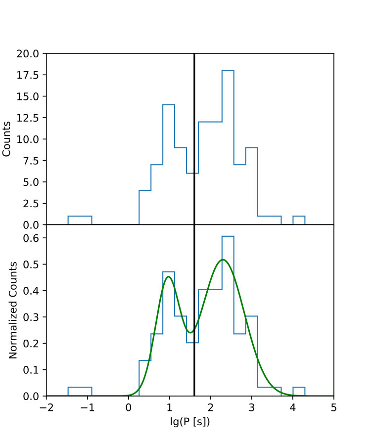 Figure 2
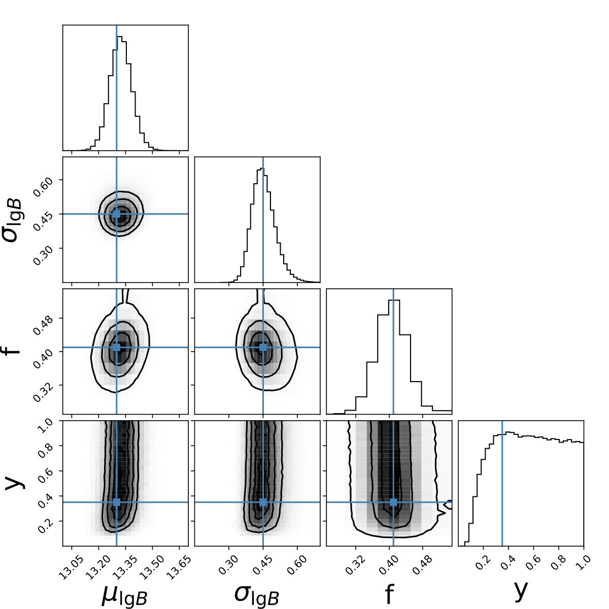 Figure 3
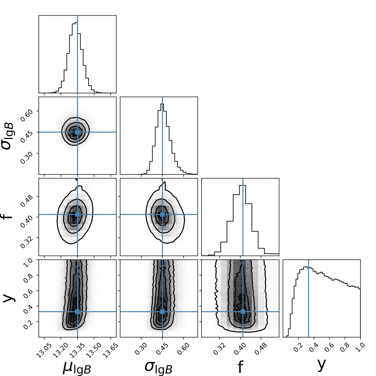 Figure 4
 Figure 5
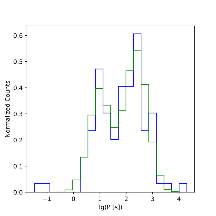 Figure 6
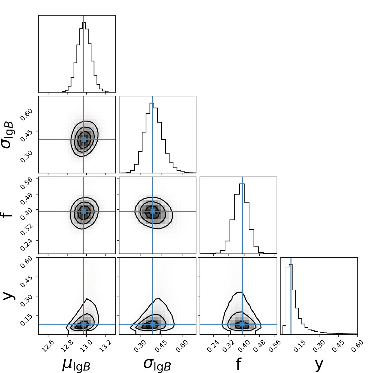 Figure 7
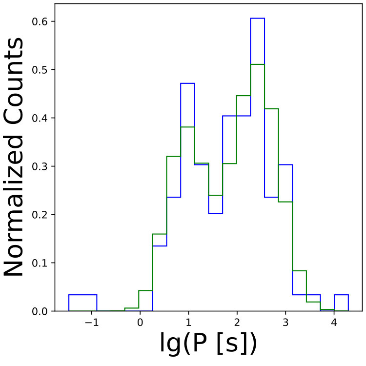 Figure 8
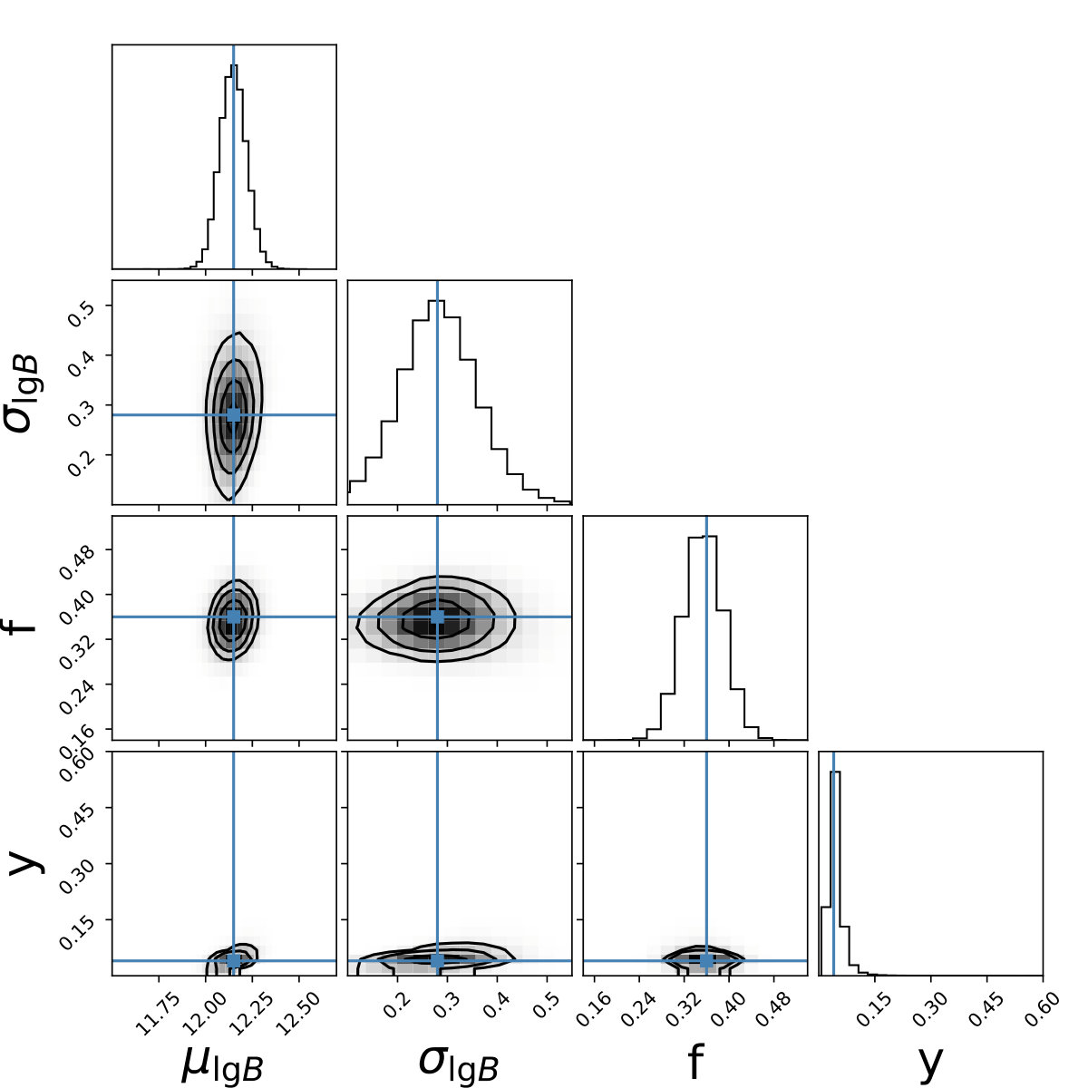 Figure 9
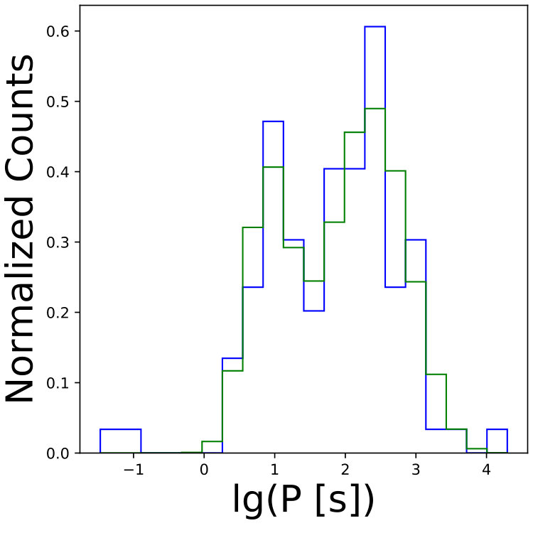 Figure 10
| 0 | 13.34 | 0.45 | 0.41 | 0.33 |
| 0.1 | 12.97 | 0.39 | 0.39 | 0.08 |
| 0.5 | 12.15 | 0.28 | 0.36 | 0.04 |
| distributions of parametersaaThe errors are given under 90% confidence level. | ||||||||
|---|---|---|---|---|---|---|---|---|
| LU | LU | U | LU | 12.97 | 0.39 | 0.39 | 0.08 | |
| U | LU | U | LU | 13.12 | 0.40 | 0.37 | 0.15 | |
| 0.1 | LU | U | U | LU | 13.10 | 0.40 | 0.37 | 0.15 |
| LU | LU | U | U | 12.87 | 0.41 | 0.40 | 0.07 | |
| LU | LU | LU | LU | 12.96 | 0.38 | 0.37 | 0.18 | |
| LU | LU | U | LU | 12.15 | 0.28 | 0.36 | 0.04 | |
| U | LU | U | LU | 12.39 | 0.35 | 0.36 | 0.08 | |
| 0.5 | LU | U | U | LU | 12.35 | 0.32 | 0.36 | 0.06 |
| LU | LU | U | U | 11.90 | 0.28 | 0.37 | 0.03 | |
| LU | LU | LU | LU | 12.15 | 0.27 | 0.36 | 0.09 | |
Peer Reviews
No public reviews on file for this paper yet. If you reviewed it on a platform where reviews are public (OpenReview, ICLR, NeurIPS, ICML), you can paste yours below so the community can read it here.
Videos
No videos yet. Explain this paper in a talk, walkthrough, or lecture? Add one.
On the bimodal spin period distribution of Be/X-ray pulsars
Xiao-Tian Xu
School of Astronomy and Space Science, Nanjing University, Nanjing 210046, China
Key Laboratory of Modern Astronomy and Astrophysics (Nanjing University), Ministry of Education, Nanjing 210046, China
Xiang-Dong Li
School of Astronomy and Space Science, Nanjing University, Nanjing 210046, China
Key Laboratory of Modern Astronomy and Astrophysics (Nanjing University), Ministry of Education, Nanjing 210046, China
Abstract
It has been reported that there are two populations of Be/X-ray pulsars, with the pulse period distribution peaked at s and s, respectively. A possible explanation of this bimodal distribution is related to different accretion modes in Be/X-ray binaries. In this work, we investigate the spin evolution of Be/X-ray pulsars based on the magnetically threaded accretion disk model. Compared with previous works, we take into account several distinct and important factors of Be/X-ray binaries, including the transient accretion behavior and possible change of the accretion disk structure during quiescence. We demonstrate that current Be/X-ray pulsars are close to the spin equilibrium determined by the balance of spin-up during outbursts and spin-down during quiescence, and that the observed bimodal distribution can be well reproduced by the equilibrium spin periods with reasonable input parameters.
accretion, accretion disks stars: emission-line, Be X-rays: binaries
††journal: ApJ††software: emcee (Foreman-Mackey et al., 2013), corner.py (Foreman-Mackey, 2016), scipy (Jones et al., 2001), R (R Core Team, 2018), diptest (Maechler, 2016)
1 Introduction
Be/X-ray binaries (BeXBs) are a sub-class of high-mass X-ray binaries, usually composed of a neutron star (NS) and an O/Be type star (Reig, 2011). The O/Be stars in BeXBs are generally fast-rotating main-sequence stars with a circumstellar disk, featured by Balmer emission lines. These observational properties can be well reproduced by the decretion disk model (Lee et al., 1991), which is similar to an accretion disk except the inverse direction of mass flow. Note that the circumstellar disk is not a stable structure, undergoing dissipation and recurrence (Haigh et al., 1999), the size and the structure of which are strongly affected by the gravity and the orbital motion of the NS (Negueruela & Okazaki, 2001; Negueruela et al., 2001; Okazaki et al., 2002). Part of the disk material is captured by the NS, preferentially near periastron. The accreted material is then channeled onto the NS surface by its magnetic field lines, so the NS usually appears as an Be/X-ray pulsar (BeXP) (Lamb et al., 1973).
BeXBs are further divided into persistent and transient sources. A small population of BeXBs are persistent sources, characterized by nearly circular orbits (with eccentricities ) and low X-ray luminosities ( erg s*-1*), while other BeXBs are transient sources with eccentric orbits (with ) (Reig, 2011). They experience outbursts from time to time, which are separated by long, quiescent intervals. There are two types of outbursts in transient BeXBs. Type I or normal outbursts are characterized by (quasi-)periodicity with peak luminosities ranging from to erg s*-1*. They are thought to be caused by rapid accretion of the NS when it passes periastron. Type II or giant outbursts show non-periodicity, and usually have peak luminosities erg s*-1*. The origin of type II outbursts is still open to debate.
Knigge et al. (2011) found that the distribution of the spin periods () of BeXPs in the Milky Way (MW) and the Small/Large Magellanic Clouds (SMC/LMC) show a bimodal feature, peaked at s and s, respectively. These authors proposed that the two populations may be related to two types of supernovae, i.e., iron core-collapse supernovae and electron-capture supernovae, respectively. Cheng et al. (2014) suggested that the two populations of BeXBs are likely associated with different accretion modes in the two types of outbursts. Because the peak luminosity and the accretion disk structure are different in type I and II outbursts, NSs undergoing different types of outbursts are subject to different accretion torques, which lead to bimodal distribution of the spin periods.
The accretion process in BeXBs is very complicated and uncertain. Although it is generally believed that the NS undergoes disk accretion during outbursts, scenarios involving wind accretion have also been proposed (Ikhsanov, 2007; Shakura et al., 2012). Even for disk accretion, there were arguments that the viscous timescale of the standard thin disk (Shakura & Sunyaev, 1973) fails to explain the observed outburst duration of type I outbursts, suggesting an advection-dominated accretion flow (ADAF) instead (Okazaki et al., 2013).
Several authors (Chashkina & Popov, 2012; Klus et al., 2014; Shi2015) investigated the long-term spin evolution of BeXPs in the SMC, and arrived the conclusion that a large population of the BeXPs are magnetars, i.e., NSs with surface magnetic fields stronger than G. But they are in conflict with the observations of cyclotron lines in the Galactic X-ray pulsars (Coburn et al., 2002; Caballero & Wilms, 2012; Walter et al., 2015, and references therein).
Considering the fact that most BeXBs are transient sources, the transition between outbursts and quiescence should play an important role in the spin evolution of the NSs. In most of the previous studies, only the long-term average evolution was taken into account, which actually deviates from the evolution in the case of transient accretion. In this work, we attempt to investigate the spin evolution in BeXPs in a more self-consistent way by considering accretion in both outbursting and quiescent stages. We take into account the possible influence of various types of outbursts and the structure of the accretion flows. In section 2, we describe our theoretical considerations. In section 3, we describe the data sample and obtain possible constraints on the model parameters through comparison with observations. We summarize our work in section 4.
2 Model
2.1 Spin evolution
We assume that the NS in a BeXB is interacting with an accretion disk originating from the Be star’s wind. We first introduce the light-cylinder radius and the inner radius of the accretion disk . Here, is defined to be
[TABLE]
where is the speed of light and is the angular velocity of NS; is evaluated by
[TABLE]
where is a factor around unity (Ghosh & Lamb, 1979a, b; Long et al., 2005), taken to be 0.5 in our work, and is the Alfvén radius for spherical accretion
[TABLE]
where is the magnetic moment of the NS, the accretion rate, the gravitational constant, and the mass of the NS, taken to be . According to the relation between and , the spin evolution is divided into two states: rotation-powered state () and accretion-powered state ()111We combine both the accretor and propeller states into the accretion-powered state since mass ejection during the propeller phase also requires extraction of accretion power..
In the rotation-powered state, the spin evolution of the NS is determined by the torque due to magnetic dipole radiation (Shapiro & Teukolsky, 1983), i.e.
[TABLE]
Considering the condition , we obtain the critical spin period that separates the rotation- and accretion-powered states,
[TABLE]
The critical spin period is much smaller than the current spin periods of most BeXPs with typical magnetic fields and accretion rates. Therefore, the rotation-powered state is usually ignorable.
In the accretion-powered state, we assume that the spin evolution of the NS is dominated by disk accretion and the interaction between the disk and the NS magnetic field, according to the magnetically threaded accretion disk model (Ghosh & Lamb, 1979a, b). The accretion torque exerted by the disk consists of two terms,
[TABLE]
Here is the material torque due to mass accretion,
[TABLE]
where is the Keplerian angular velocity in the disk, and is the torque resulting from the magnetic field-disk interaction, due to the shearing motion between the magnetic field lines of the NS and the disk material. Equation (6) can be expressed in the following form (Ghosh & Lamb, 1979a, b),
[TABLE]
where is the fastness parameter defined by
[TABLE]
and is a dimensionless function, which is, according to Ghosh & Lamb (1979a, b),
[TABLE]
This equation was derived based on the assumption that the NS magnetic field penetrates the disk via the Kelvin-Helmholtz instability, turbulent diffusion, and reconnection with small-scale fields within the disk. However, Wang (1987) pointed out that this will lead to the pressure of the wound field to exceed the thermal pressure at large radius and disrupt the disk. There are various forms of the function proposed in the literature (e.g., Wang, 1995; Li & Wang, 1996; Kluźniak & Rappaport, 2007). Here we adopt the following simplified equation
[TABLE]
which is similar to the torque equation in Lipunov (1982) and used in previous studies (e.g. Li, 1999; Hartmann, 2002; Ho et al., 2014; Ekşi et al., 2015). In Eq. (11), is a critical value of the fastness parameter at which . This means that when and when . Also note that Eq. (11) can be used to cover both accretor and propeller states: when , ; when , .
It should be pointed out that Eq. (8) is only applicable to steady accretion onto NSs, while the accretion processes in BeXBs are much more complicated, so we consider further modifications of the accretion torque by taking into the following factors.
(1) Due to the shear between the magnetosphere of the NS and the accretion disk, there is an open-field region on the magnetosphere, where the accreting material can potentially escape as wind (Lovelace et al., 1995; Romanova et al., 2003). The coupling between the magnetic field of the NS and the wind material generates a spin-down torque on the NS. In our model, we assume that a fraction of the accreting material leaves the system as wind, i.e., . Then, the torque exerted by the wind is given by
[TABLE]
where is the Alfvén radius of the wind, and is a efficiency coefficient for the magnetic field-wind interaction. In our work, we take . Then, the total torque becomes
[TABLE]
(2) Most BeXBs are transient sources subject to (quasi-)periodic type I outbursts (Reig, 2011). The spin evolution during type I outbursts is described by
[TABLE]
where the subscripts I represents the parameters evaluated for type I outbursts. Assuming that the detection of X-ray pulsations marks the occurrence of the outburst phase, we derive that the duty cycle of type I outbursts roughly ranges from 0.005 to 0.05 from the data sample compiled by Yang et al. (2017) .
(3) Type II outbursts are rare but more violent compared with type I outbursts. The origin and accretion physics of type II outbursts are still open to debate. While Okazaki et al. (2013) argued that the Bondi-Hoyle-Lyttleton accretion is responsible for type II outbursts, disk accretion seems to be observationally preferred (e.g., Haigh et al., 1999; Sugizaki et al., 2017). Here we adopt the suggestion by Sugizaki et al. (2017) and write the torque during type II outbursts to be
[TABLE]
where the subscript II represents that the parameters are evaluated for type II outbursts. We introduce the duty cycle to describe the occurrence of type II outburst, given by
[TABLE]
The observations by Sugizaki et al. (2017) suggest that is about 0.1 with the outburst rate and the outburst duration .
(4) During the quiescent phase BeXBs are very faint with X-ray luminosities as low as (Yang et al., 2017), so the accretion disk may evolve from an optically thick, geometrically thin disk to an ADAF. Consequently, the accretion disk becomes geometrically thick with sub-Keplerian rotation, so we add a parameter to modify the disk rotation for an ADAF,
[TABLE]
The typical value of is (Narayan & Yi, 1995). Then,the torque in the quiescent phase can be rewritten to be
[TABLE]
where the subscript q represents the parameters evaluated in the quiescent phases.
With the above factors taken into account, the averaged total torque exerted by an accretion disk is written to be
[TABLE]
Combining Eqs. (6)-(19) and setting , we obtain an approximate estimate of the equilibrium spin period for the NS in a transient BeXB (see Appendix for the derivation),
[TABLE]
where
[TABLE]
In addition, we require that the magnitude of the spin-down torque generated by the wind is always weaker than that of the material torque, that is .
2.2 Spin-change timescale and spin equilibrium
In the accretion-powered state, the spin evolution of the NS is determined by the total torque exerted on the NS by the accretion disk
[TABLE]
where is the moment of inertia of the NS and is the derivative of the spin period. This equation can be solved analytically, and according to its solution, we obtain an estimate of the typical spin-change timescale (see Appendix for the derivation),
[TABLE]
where is converted into via
[TABLE]
is the radius of the NS, and is the averaged X-ray luminosity, defined by
[TABLE]
It is interesting to note that is independent on the structure of the accretion disk and the wind loss, though these two factors affect the value of . Eq. (23) shows that , i.e., systems with higher average accretion rate and stronger magnetic field can reach spin equilibrium with shorter time. Assuming steady accretion and adopting the following parameters: , , erg s*-1*, G cm3, cm, , g cm2, , and , we obtain yr, which implies that a typical NS is able to reach the spin equilibrium within even if we only take into account accretion during quiescence. Obviously become shorter if we consider the contribution from type I/II outbursts. Considering the ages of most BeXBs are roughly 10 Myr (Antoniou et al., 2010), it is safe to assume that most of observed BeXPs have evolved to be near the spin equilibrium.
We then perform a numerical test of the above analysis. We adopt the following parameters: s, , G cm3, cm, or 1, or 0.005, or 0.1, days, or 0.1, and . Our results are shown in Fig. 1. In this figure, the upper and lower panels depict the results with and , respectively. In the first, second, third, and fourth columns, we set to be , , , and , respectively. In each panel, the blue line represents the evolutionary track of , the black vertical line the age of yr, and the black horizontal line the equilibrium spin period given by Eq. (20). The numerical calculations confirm our analytical result that current BeXPs should be close to spin equilibrium. A remarkable feature is that type II outbursts can significantly change the overall distribution of the equilibrium spin periods. Cheng et al. (2014) showed that the BeXPs with s are more likely to experience type II outbursts compared with those with s. The calculated results presented in Fig. 1 demonstrates that the NSs can be significantly spun up during type II outbursts.
In next section we perform statistical calculations to examine whether the equilibrium spin periods in transient accretion can reproduce the bimodal distribution of BeXPs.
3 The bimodal distribution
We first describe the data sample that will be used to compare with the model prediction. There are 103 BeXPs in the sample, including the sources from MW, SMC, and LMC (data taken from Raguzova & Popov, 2005; Reig, 2011; Townsend et al., 2011; Sturm et al., 2012; Vasilopoulos et al., 2014; Coe & Kirk, 2015; Vasilopoulos et al., 2016, 2017; Yang et al., 2017). The distribution of the pulse period is presented in Fig. 2, where the black vertical line represents s. The upper panel shows the histogram of the real distribution, and the lower panel depicts the normalized distribution of (blue solid line) and the fitted curve (green solid line)222 The fitting process was performed with the Scipy library (Jones et al., 2001). with a double-Gaussian function, which is defined as
[TABLE]
The fitting parameters are as follows
;
, ;
, ,
where , , and are in the units of second, and the error for each parameter was calculated by the fitting method333See https://docs.scipy.org/doc/scipy/reference/generated/scipy.optimize.curve_fit.html for details.. We apply the Hartigans’ dip test (Hartigan & Hartigan, 1985) to our sample. The P-value is 0.4308 for the distribution in logarithmic scale, and 0.9918 in linear scale444The Hartigans’ dip test was performed with the R based library diptest (Maechler, 2016; R Core Team, 2018).
Then, we introduce the properties of the input parameters for our statistical calculation,
- •
The duty cycle of type I outbursts: based on the data compiled in Yang et al. (2017) for the occurrence of X-ray outbursts and detection of X-ray pulsations, we adopt a log-uniform distribution in the range of ;
- •
The X-ray luminosity during type I outbursts: we adopt a log-uniform distribution in the range of erg s*-1* (Reig, 2011);
- •
The X-ray luminosity during type II outbursts: Cheng et al. (2014) showed that the peak X-ray luminosity of the BeXPs is truncated around , and the distribution seems to prefer high-luminosity end. We accordingly adopt a uniform distribution in the range of erg s*-1*.
- •
The X-ray luminosity in the quiescent phase : we adopt a log-uniform distribution in the range of erg s*-1* (Yang et al., 2017);
- •
The critical value of the fastness parameter : various studies show that it is in the range of (Ghosh & Lamb, 1979a, b; Wang, 1995; Li & Wang, 1996; Long et al., 2005; Zanni & Ferreira, 2009, 2013). In our work, we adopt a uniform distribution in the range of ;
- •
The ADAF parameter : we adopt a uniform distribution in the the range (Narayan & Yi, 1995);
In next section we will vary the distribution forms and examine their influence. Other (free) parameters are listed as follows,
- •
The disk wind fraction ;
- •
The NS magnetic fields : we adopt a log-normal distribution for , i.e.
[TABLE]
where the average value and the variance are left as free parameters;
- •
The fraction of BeXPs that undergo type II outbursts;
- •
The duty cycle of type II outbursts.
With the above parameters and the equilibrium spin period assumption we model the bimodal distribution of BeXPs with a Markov Chain Monte-Carlo method555The calculations were made with the emcee code, which is an open-source software for the Markov Chain Monte-Carlo method (Foreman-Mackey et al., 2013).. We consider three types of solutions in our model: the no-wind solution with , the weak-wind solution with , and the strong-wind solution with (hereafter Solution-1, Solution-2, and Solution-3, respectively). The calculated results are shown in Fig. 3 666The corner plots were generated by the corner.py module written by Foreman-Mackey (2016).. There are three rows and two columns in each figure. The first, second, and third rows present the results of Solution-1, Solution-2, and Solution-3. The left column presents the posterior probability distribution of , , , and , where the blue solid lines represent the best fitting points, and the right column presents the comparison between the observed distribution (blue solid lines) and the model distribution (green solid lines) with the best fitting parameters, which are summarized in Table 1.
It is seen from Fig. 3 and Table 1 that the three solutions can well reproduce the bimodal distribution of the spin periods. The short-period subpopulation mainly consists of BeXBs which undergo type II outbursts. There is a tendency that , , and all become smaller with increasing . This is not difficult to understand. As the wind torque acts to spin down the NS, a weaker magnetic field is required with stronger wind, given a specific equilibrium spin period. When increases from 0 to 0.5, the average value of decreases from 13.34 ( G) to 12.15 ( G), which are still in the reasonable range for X-ray pulsars. The fraction of BeXBs with type II outbursts varies from 0.41 to 0.36. According to the data in Cheng et al. (2014) we infer that the observed value of for transient BeXBs is roughly 0.2. But this should be taken as a lower limit since type II outbursts must have been missed because of limited monitoring by X-ray telescopes. The duty cycle of type II outbursts changes from 0.33 to 0.04, which is roughly consistent with the observed value .
We mention that the derived parameter distributions depend on the values of the input parameters which are subject to some uncertainties. For example, in our calculation, we use a constant luminosity during outbursts and ignore its evolution during the rising and decay phases for simplicity. The adopted distributions of , , and are somewhat speculative and need to be refined by more dense observations. In addition, we neglect the possible influence of the eccentricities in BeXBs and the possible dependence of on both the orbital period and the eccentricity. To see how the specific distribution functions of the input parameters potentially affect our results, we compare the results by taking into account different combinations of the distribution functions, with LU for log-uniform and U for uniform distributions. In the cases of Solution-2 and Solution-3, and we consider the following combinations for for ,: (LU, LU, U, LU), (U, LU, U, LU), (LU, U, U, LU, U), (LU, LU, U, U), and (LU, LU, LU, LU). Our results are summarized in Table 2. We see that in these different combinations we obtain results that are compatible with each other. Therefore, our results are not sensitively dependent on the adopted distribution functions.
4 Conclusions
We summarize our work as follows.
(1) NSs in most BeXBs undergo spin-up during outbursts and spin-down during quiescence, so their spin evolution is controlled by the competition between the spin-up and spin-down torques. Therefore, it is inappropriate to use long-term, average steady accretion to calculate the spin evolution and derive the magnetic fields of the accreting NSs.
(2) Most NSs in BeXBs have reached the equilibrium spin periods since the spin-change timescale is sufficiently short compared with the ages of BeXBs.
(3) Considering the transient behavior of BeXBs, it seems able to reproduce the bimodal spin period distribution with the assumption of the equilibrium spin period for NSs with typical magnetic fields ( G). The critical factors that determine the spin period distribution are the properties of type I and II outbursts.
This work was supported by the National Key Research and Development Program of China (2016YFA0400803), the Natural Science Foundation of China under grant Nos. 11333004, 11773015, 11573016, and Project U1838201 supported by NSFC and CAS.
Appendix A Detailed derivation of and
[TABLE]
Here we define two parameters and , which are respectively given by
[TABLE]
and
[TABLE]
Then, Eq. (A1) can be rewritten as
[TABLE]
The equilibrium spin is given by setting , i.e.,
[TABLE]
Assuming that the torque generated by the wind is smaller than the material toque, mathematically and , we have . Then, Eq. (A4) has following solution
[TABLE]
where is the evolutionary time, and is the spin period at . Note that, according to Eq. (A5), can be substituted by . Then, the spin evolution is given by
[TABLE]
According to the exponential term in Eq. (A7), we can define the spin-evolutionary timescale ,
[TABLE]
The reference list from the paper itself. Each links out to its DOI / PubMed record.
- 1Antoniou et al. (2010) Antoniou, V., Zezas, A., Hatzidimitriou, D., & Kalogera, V. 2010, Ap J, 716, L 140
- 2Caballero & Wilms (2012) Caballero, I., & Wilms, J. 2012, Mem. Soc. Astron. Italiana, 83, 230
- 3Chashkina & Popov (2012) Chashkina, A., & Popov, S. B. 2012, New A, 17, 594
- 4Cheng et al. (2014) Cheng, Z.-Q., Shao, Y., & Li, X.-D. 2014, Ap J, 786, 128
- 5Coburn et al. (2002) Coburn, W., Heindl, W. A., Rothschild, R. E., et al. 2002, Ap J, 580, 394
- 6Coe & Kirk (2015) Coe, M. J., & Kirk, J. 2015, MNRAS, 452, 969
- 7Ekşi et al. (2015) Ekşi, K. Y., Andaç, İ. C., Çıkıntoğlu, S., et al. 2015, MNRAS, 448, L 40
- 8Foreman-Mackey (2016) Foreman-Mackey, D. 2016, The Journal of Open Source Software, 24, doi:10.21105/joss.00024. http://dx.doi.org/10.5281/zenodo.45906 · doi ↗