Change-point Detection by the Quantile LASSO Method
Gabriela Ciuperca, Mat\'u\v{s} Maciak

TL;DR
This paper introduces a quantile LASSO method for change-point detection in piece-wise constant models that is robust to heavy-tailed errors and can estimate multiple quantiles simultaneously.
Contribution
The paper presents a novel quantile LASSO approach for change-point detection that does not require traditional distributional assumptions and provides consistent change-point estimates.
Findings
The method effectively handles heavy-tailed error distributions.
It provides consistent estimates when the number of change-points is correctly identified.
Numerical simulations demonstrate robustness and empirical performance.
Abstract
A simultaneous change-point detection and estimation in a piece-wise constant model is a common task in modern statistics. If, in addition, the whole estimation can be performed automatically, in just one single step without going through any hypothesis tests for non-identifiable models, or unwieldy classical a-posterior methods, it becomes an interesting, but also challenging idea. In this paper we introduce the estimation method based on the quantile LASSO approach. Unlike standard LASSO approaches, our method does not rely on typical assumptions usually required for the model errors, such as sub-Gaussian or Normal distribution. The proposed quantile LASSO method can effectively handle heavy-tailed random error distributions, and, in general, it offers a more complex view of the data as one can obtain any conditional quantile of the target distribution, not just the conditional mean.…
Click any figure to enlarge with its caption.
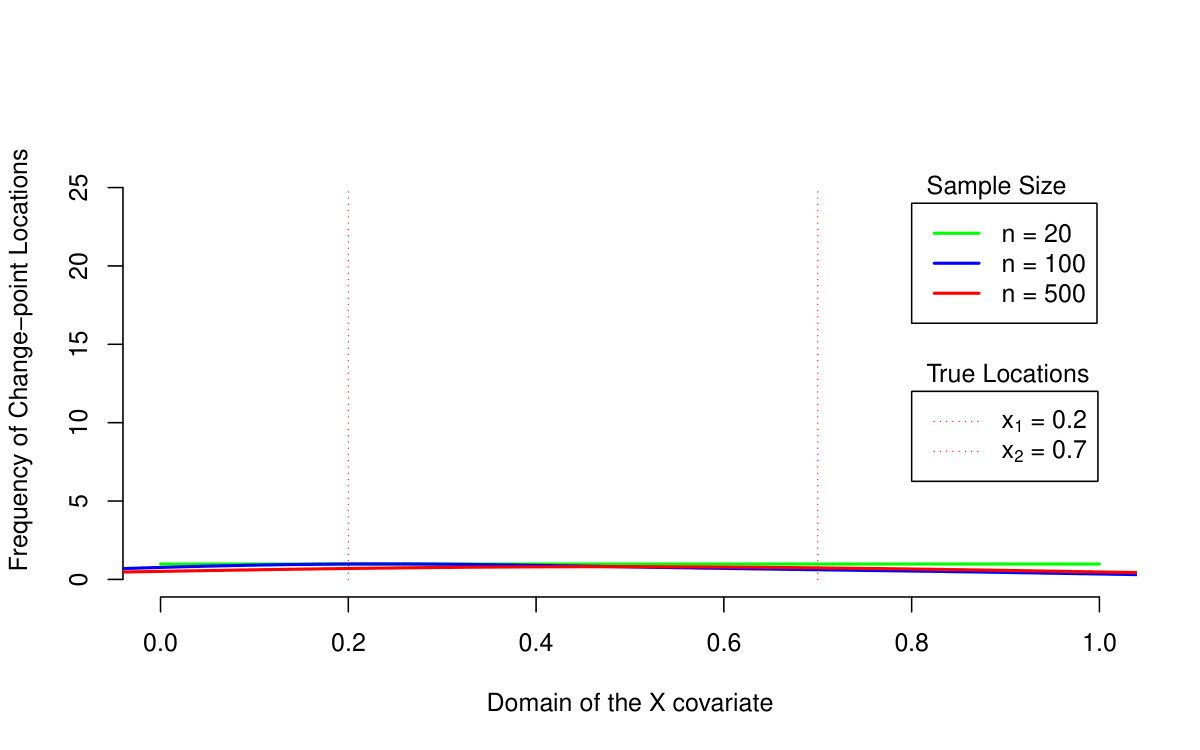 Figure 1
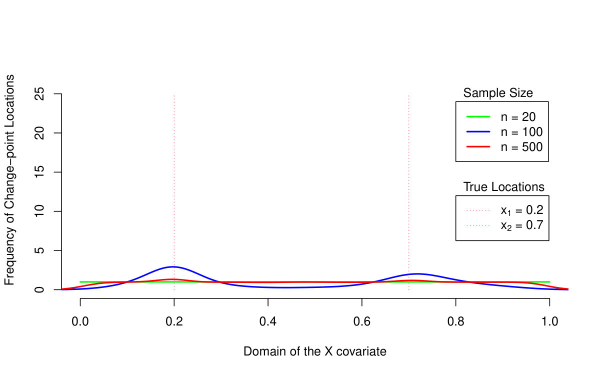 Figure 2
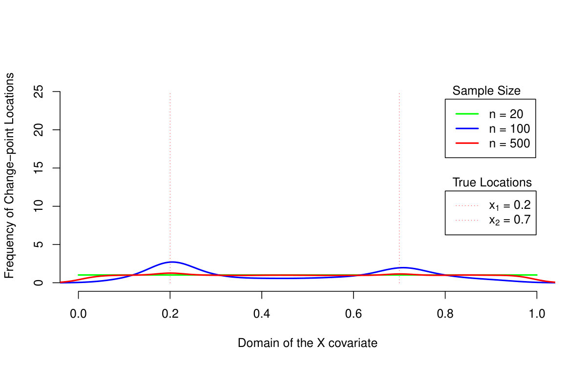 Figure 3
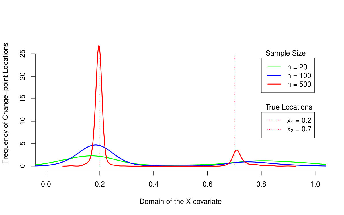 Figure 1
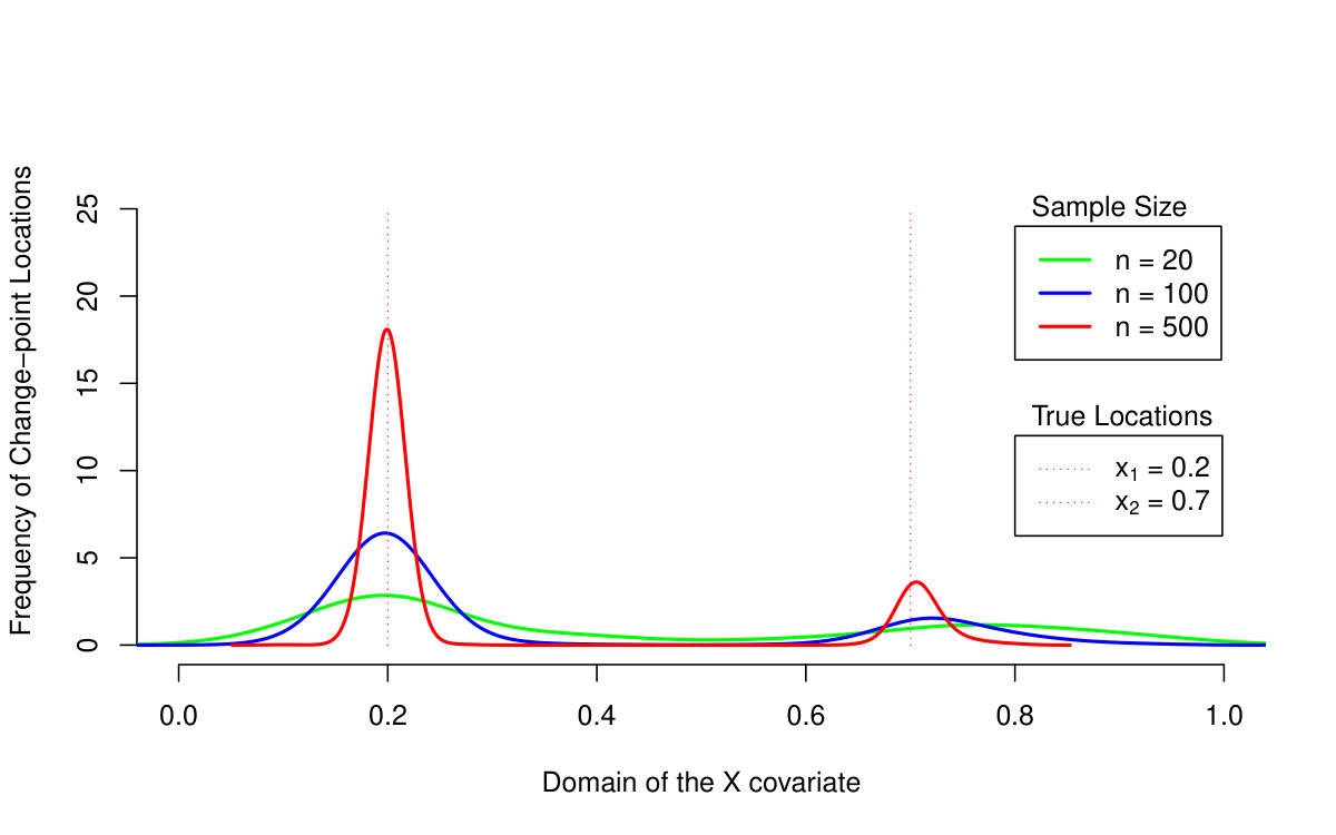 Figure 2
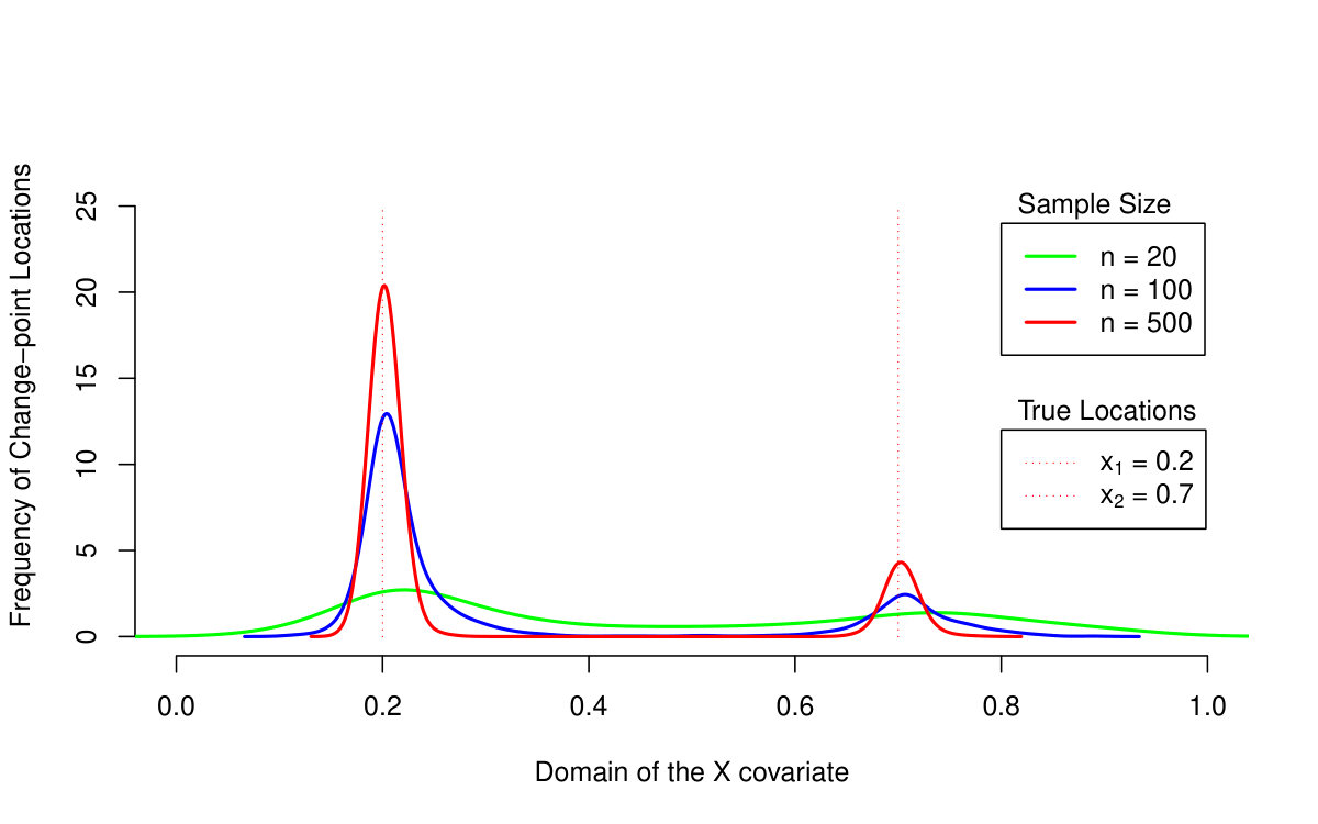 Figure 3
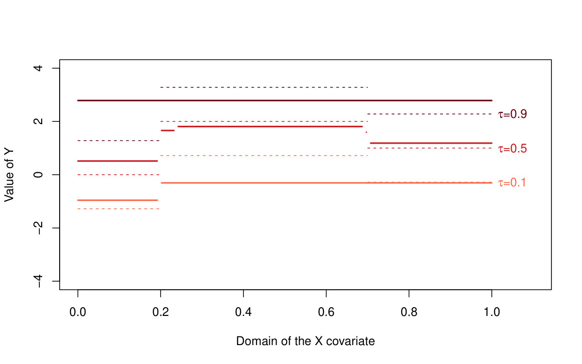 Figure 7
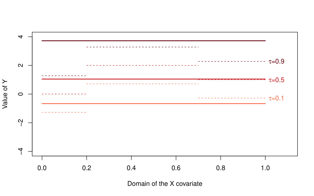 Figure 8
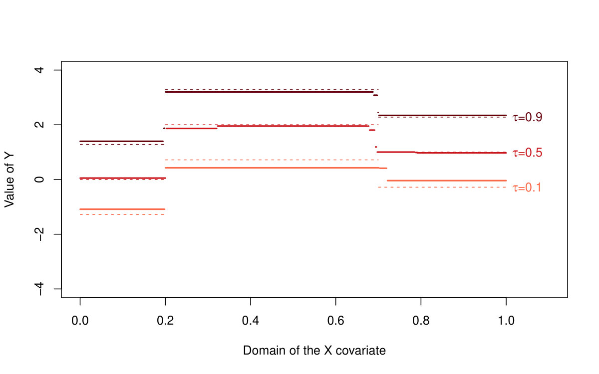 Figure 9
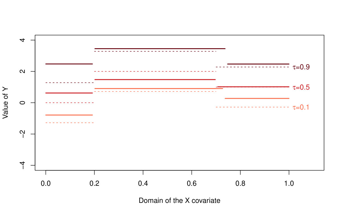 Figure 10
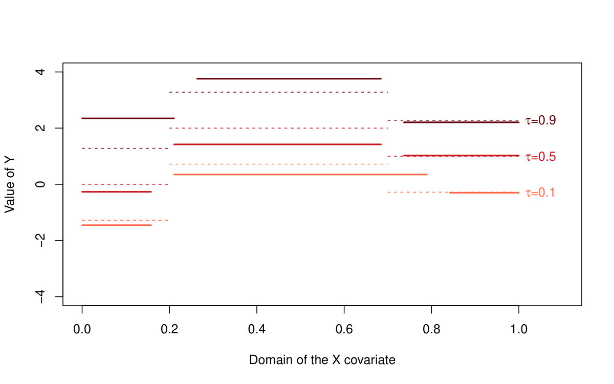 Figure 11
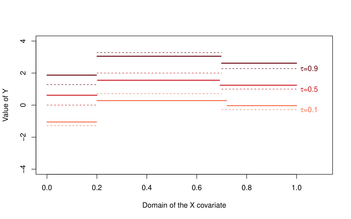 Figure 12
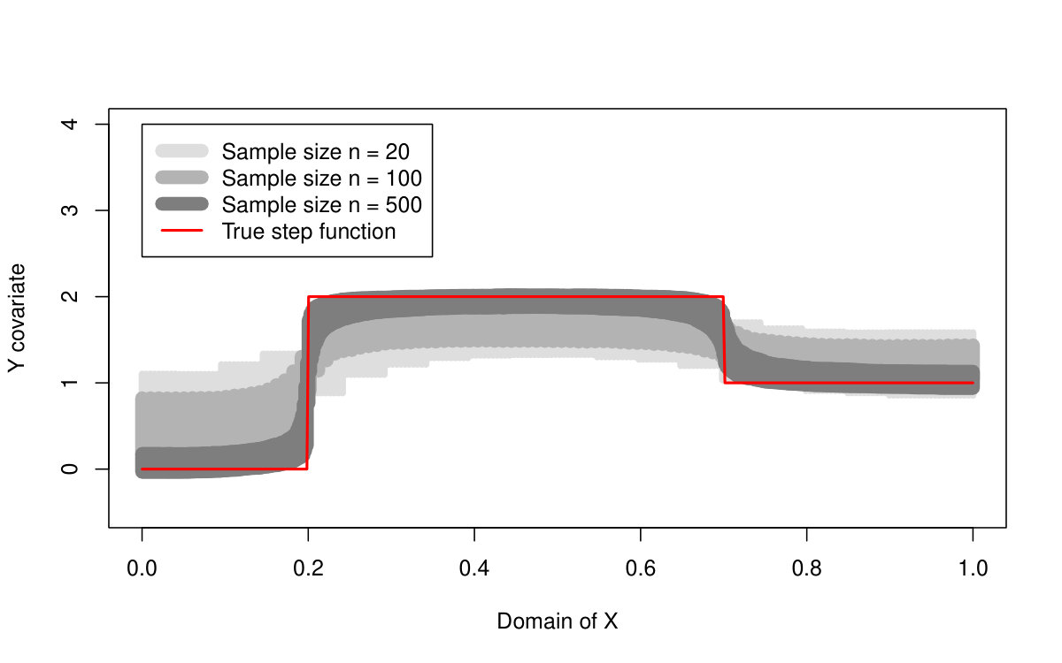 Figure 13
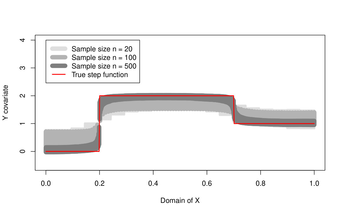 Figure 14
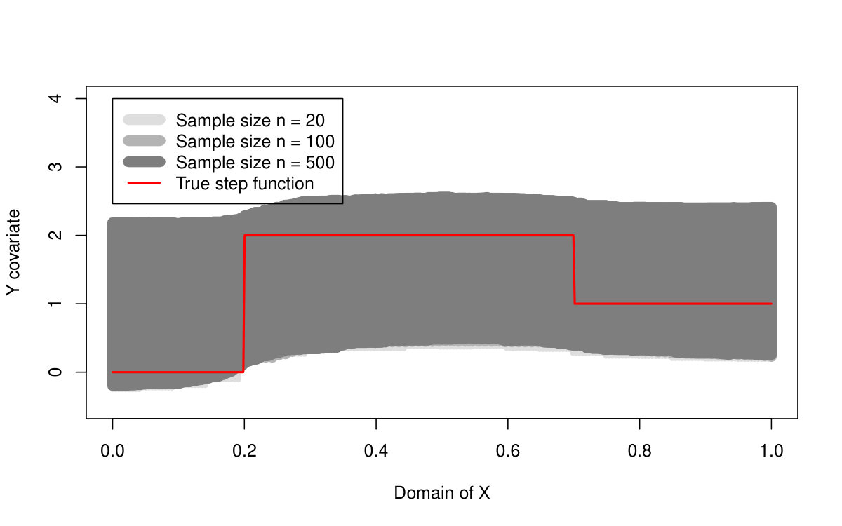 Figure 15
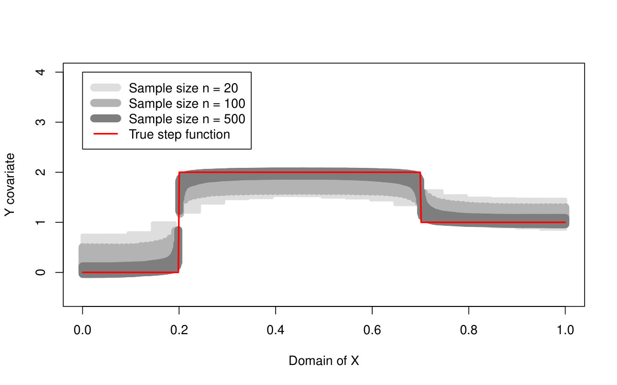 Figure 16
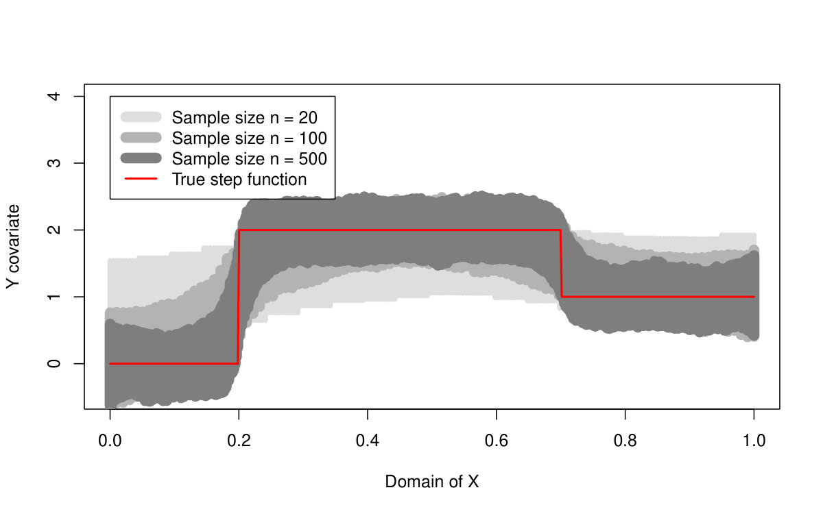 Figure 17
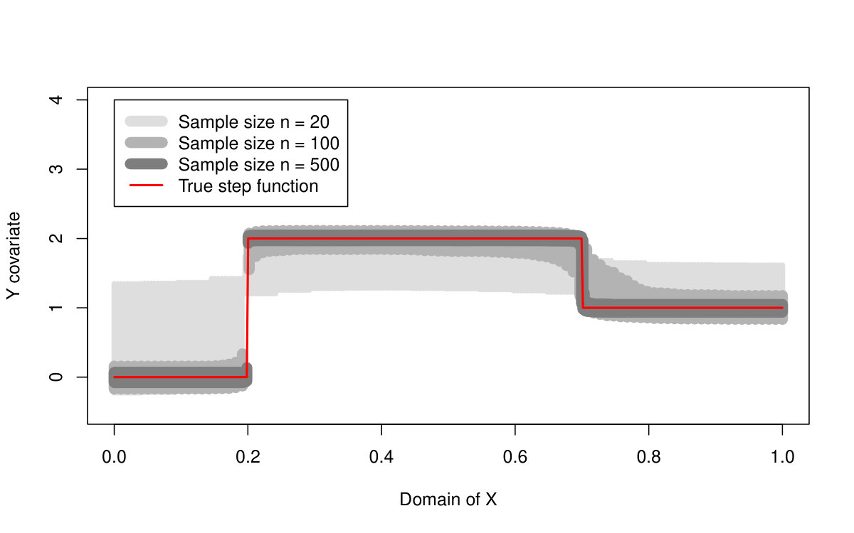 Figure 18
| Model with | Model with | ||||||||||||
|---|---|---|---|---|---|---|---|---|---|---|---|---|---|
|
Value |
Mean |
Std.Err. |
Est. Bias |
MSE |
Est. Bias |
MSE |
[M M M] |
||||||
| 20 | 0.05 | 3.87 | 0.30 | (0.09) | -0.32 | (0.41) | 0.66 | (0.35) | 0.49 | (0.46) | 1.06 | (0.55) | [000] |
| 0.10 | 3.87 | 0.56 | (0.18) | -0.02 | (0.40) | 0.55 | (0.28) | 0.39 | (0.39) | 0.92 | (0.38) | [000] | |
| 0.25 | 3.87 | 1.08 | (0.29) | 0.03 | (0.33) | 0.45 | (0.24) | 0.20 | (0.33) | 0.76 | (0.21) | [000] | |
| 0.50 | 3.87 | 1.47 | (0.46) | -0.01 | (0.31) | 0.52 | (0.22) | -0.04 | (0.30) | 0.70 | (0.13) | [000] | |
| 0.75 | 3.87 | 1.04 | (0.18) | -0.03 | (0.32) | 0.56 | (0.27) | -0.21 | (0.32) | 0.76 | (0.23) | [000] | |
| 0.90 | 3.87 | 0.52 | (0.17) | 0.07 | (0.41) | 0.80 | (0.35) | -0.33 | (0.40) | 0.88 | (0.40) | [000] | |
| 0.95 | 3.87 | 0.28 | (0.09) | 0.34 | (0.44) | 1.04 | (0.45) | -0.40 | (0.49) | 1.01 | (0.60) | [000] | |
| 100 | 0.05 | 2.15 | 1.67 | (0.57) | 0.19 | (0.25) | 0.45 | (0.22) | 0.31 | (0.26) | 0.61 | (0.27) | [016] |
| 0.10 | 2.15 | 2.63 | (0.85) | 0.17 | (0.20) | 0.40 | (0.17) | 0.09 | (0.19) | 0.31 | (0.14) | [1310] | |
| 0.25 | 2.15 | 4.73 | (1.31) | 0.10 | (0.15) | 0.35 | (0.13) | 0.00 | (0.14) | 0.14 | (0.07) | [1615] | |
| 0.50 | 2.15 | 6.22 | (1.51) | -0.01 | (0.14) | 0.41 | (0.15) | -0.01 | (0.13) | 0.12 | (0.06) | [2921] | |
| 0.75 | 2.15 | 4.40 | (0.91) | -0.12 | (0.16) | 0.44 | (0.18) | 0.00 | (0.14) | 0.16 | (0.09) | [1615] | |
| 0.90 | 2.15 | 2.29 | (0.45) | -0.19 | (0.19) | 0.56 | (0.19) | -0.17 | (0.19) | 0.53 | (0.18) | [039] | |
| 0.95 | 2.15 | 1.36 | (0.27) | -0.20 | (0.22) | 0.64 | (0.20) | -0.37 | (0.22) | 0.80 | (0.18) | [003] | |
| 500 | 0.05 | 1.11 | 7.73 | (2.51) | 0.24 | (0.13) | 0.41 | (0.15) | -0.06 | (0.09) | 0.10 | (0.03) | [71525] |
| 0.10 | 1.11 | 12.82 | (4.44) | 0.19 | (0.10) | 0.36 | (0.13) | -0.06 | (0.07) | 0.09 | (0.03) | [152441] | |
| 0.25 | 1.11 | 22.60 | (6.33) | 0.10 | (0.07) | 0.33 | (0.11) | -0.04 | (0.06) | 0.10 | (0.02) | [375369] | |
| 0.50 | 1.11 | 30.23 | (6.61) | -0.01 | (0.06) | 0.38 | (0.13) | 0.00 | (0.05) | 0.09 | (0.02) | [5579103] | |
| 0.75 | 1.11 | 20.26 | (3.35) | -0.13 | (0.08) | 0.41 | (0.15) | 0.04 | (0.06) | 0.10 | (0.02) | [385371] | |
| 0.90 | 1.11 | 9.95 | (1.07) | -0.23 | (0.10) | 0.52 | (0.17) | 0.06 | (0.08) | 0.09 | (0.03) | [142440] | |
| 0.95 | 1.11 | 5.52 | (0.79) | -0.27 | (0.13) | 0.58 | (0.18) | 0.06 | (0.09) | 0.10 | (0.04) | [61527] | |
| Model with | Model with | Model w. SMUCE | ||||||||||||
|---|---|---|---|---|---|---|---|---|---|---|---|---|---|---|
|
Est. Bias |
MSE |
Est. Bias |
MSE |
Est. Bias |
MSE | |||||||||
| SLasso | 20 | 0.00 | (0.23) | 0.43 | (0.16) | 0.00 | (0.23) | 0.65 | (0.08) | 0.00 | (0.23) | 0.27 | (0.15) | |
| 100 | 0.00 | (0.10) | 0.35 | (0.12) | 0.00 | (0.10) | 0.09 | (0.04) | 0.00 | (0.10) | 0.13 | (0.08) | ||
| 500 | 0.00 | (0.04) | 0.33 | (0.11) | 0.00 | (0.04) | 0.06 | (0.02) | 0.00 | (0.04) | 0.02 | (0.01) | ||
| 20 | -0.01 | (0.31) | 0.53 | (0.21) | -0.04 | (0.29) | 0.70 | (0.13) | 0.00 | (0.24) | 0.31 | (0.17) | ||
| 100 | -0.01 | (0.14) | 0.43 | (0.14) | 0.00 | (0.13) | 0.12 | (0.06) | 0.00 | (0.13) | 0.20 | (0.11) | ||
| QLasso | 500 | -0.01 | (0.06) | 0.40 | (0.12) | 0.00 | (0.05) | 0.09 | (0.02) | 0.00 | (0.05) | 0.03 | (0.01) | |
| SMUCE | 20 | -0.01 | (0.23) | 0.55 | (0.21) | |||||||||
| 100 | 0.01 | (0.10) | 0.12 | (0.10) | ||||||||||
| 500 | 0.00 | (0.04) | 0.02 | (0.01) | ||||||||||
| SLasso | 20 | 0.00 | (0.38) | 0.61 | (0.46) | 0.00 | (0.38) | 0.73 | (0.36) | 0.00 | (0.38) | 0.47 | (0.31) | |
| 100 | 0.00 | (0.17) | 0.41 | (0.14) | 0.00 | (0.17) | 0.33 | (0.81) | 0.00 | (0.17) | 0.20 | (0.11) | ||
| 500 | 0.00 | (0.08) | 0.36 | (0.11) | 0.00 | (0.08) | 0.69 | (2.32) | 0.00 | (0.08) | 0.05 | (0.03) | ||
| 20 | -0.01 | (0.35) | 0.59 | (0.28) | -0.04 | (0.34) | 0.73 | (0.16) | 0.01 | (0.28) | 0.39 | (0.21) | ||
| 100 | -0.01 | (0.15) | 0.44 | (0.14) | 0.00 | (0.14) | 0.15 | (0.08) | 0.00 | (0.14) | 0.24 | (0.12) | ||
| QLasso | 500 | -0.02 | (0.07) | 0.42 | (0.13) | 0.00 | (0.06) | 0.11 | (0.03) | 0.00 | (0.06) | 0.04 | (0.02) | |
| SMUCE | 20 | -0.01 | (0.39) | 1.33 | (2.06) | |||||||||
| 100 | 0.01 | (0.19) | 1.08 | (1.60) | ||||||||||
| 500 | 0.00 | (0.09) | 0.95 | (2.52) | ||||||||||
| SLasso | 20 | -1.57 | (74.19) | 5867 | (154600) | -1.57 | (74.19) | 109736 | (3089261) | -1.57 | (74.19) | 5785 | (154589) | |
| 100 | -1.15 | (22.21) | 524 | (7333) | -1.15 | (22.21) | 50589 | (765657) | -1.15 | (22.21) | 512 | (7322) | ||
| 500 | -1.65 | (36.73) | 1354 | (24483) | -1.65 | (36.72) | 671194 | (12245127) | -1.65 | (36.72) | 1353 | (24477) | ||
| 20 | -0.02 | (0.46) | 0.75 | (0.48) | -0.03 | (0.44) | 0.81 | (0.30) | 0.01 | (0.36) | 0.53 | (0.30) | ||
| 100 | -0.02 | (0.20) | 0.49 | (0.16) | -0.02 | (0.18) | 0.20 | (0.12) | -0.01 | (0.18) | 0.28 | (0.15) | ||
| QLasso | 500 | -0.02 | (0.09) | 0.44 | (0.14) | 0.00 | (0.08) | 0.18 | (0.06) | 0.00 | (0.07) | 0.05 | (0.03) | |
| SMUCE | 20 | -1.58 | (74.19) | 109953 | (3091453) | |||||||||
| 100 | -1.16 | (22.21) | 50683 | (766016) | ||||||||||
| 500 | -1.65 | (36.72) | 671259 | (12245434) | ||||||||||
| Number of Jumps | Change-point Detection Error | ||||||||||||
|---|---|---|---|---|---|---|---|---|---|---|---|---|---|
| Value | Avg. | Avg. |
/
SMUCE |
(with ) | (with ) |
(/
SMUCE |
|||||||
| SLasso | 20 | 3.87 | 1.68 | 0.98 | [003] | [0011] | 0.08 | (0.06) | 0.17 | (0.03) | 0.04 | (0.04) | |
| 100 | 2.15 | 7.77 | 3.29 | [2214] | [2221] | 0.02 | (0.02) | 0.01 | (0.01) | 0.01 | (0.01) | ||
| 500 | 1.11 | 38.09 | 4.54 | [323266] | [3323] | 0.00 | (0.00) | 0.00 | (0.00) | 0.00 | (0.00) | ||
| 20 | 3.87 | 1.58 | 1.17 | [000] | [0013] | 0.10 | (0.07) | NaN | (NA) | 0.04 | (0.04) | ||
| 100 | 2.15 | 6.54 | 4.00 | [2221] | [1128] | 0.03 | (0.04) | 0.01 | (0.01) | 0.01 | (0.03) | ||
| QLasso | 500 | 1.11 | 31.31 | 4.68 | [353570] | [4465] | 0.00 | (0.00) | 0.00 | (0.00) | 0.00 | (0.00) | |
| SMUCE | 20 | [004] | 0.07 | (0.04) | |||||||||
| 100 | [014] | 0.02 | (0.03) | ||||||||||
| 500 | [223] | 0.00 | (0.00) | ||||||||||
| SLasso | 20 | 3.87 | 2.14 | 2.25 | [005] | [009] | 0.10 | (0.06) | 0.12 | (0.06) | 0.06 | (0.05) | |
| 100 | 2.15 | 8.86 | 4.02 | [3323] | [1114] | 0.05 | (0.05) | 0.02 | (0.02) | 0.02 | (0.03) | ||
| 500 | 1.11 | 41.10 | 7.61 | [6767124] | [3323] | 0.01 | (0.02) | 0.00 | (0.00) | 0.00 | (0.00) | ||
| 20 | 3.87 | 1.52 | 1.55 | [000] | [0013] | 0.11 | (0.06) | NaN | (NA) | 0.05 | (0.05) | ||
| 100 | 2.15 | 6.03 | 3.91 | [2220] | [0026] | 0.04 | (0.05) | 0.01 | (0.02) | 0.02 | (0.04) | ||
| QLasso | 500 | 1.11 | 28.98 | 4.59 | [5454104] | [4436] | 0.01 | (0.01) | 0.00 | (0.00) | 0.00 | (0.00) | |
| SMUCE | 20 | [006] | 0.09 | (0.05) | |||||||||
| 100 | [0210] | 0.05 | (0.05) | ||||||||||
| 500 | [2223] | 0.02 | (0.02) | ||||||||||
| SLasso | 20 | 3.87 | 112.40 | 83.71 | [0017] | [0119] | 0.12 | (0.06) | 0.08 | (0.06) | 0.10 | (0.06) | |
| 100 | 2.15 | 386.53 | 237.47 | [7796] | [0096] | 0.12 | (0.06) | 0.01 | (0.01) | 0.07 | (0.06) | ||
| 500 | 1.11 | 1414.77 | 1353.09 | [164164493] | [00499] | 0.10 | (0.06) | 0.00 | (0.00) | 0.08 | (0.06) | ||
| 20 | 3.87 | 1.45 | 2.66 | [001] | [0012] | 0.12 | (0.06) | 0.07 | (NA) | 0.06 | (0.05) | ||
| 100 | 2.15 | 5.27 | 3.65 | [2222] | [0039] | 0.05 | (0.05) | 0.02 | (0.02) | 0.03 | (0.04) | ||
| QLasso | 500 | 1.11 | 24.58 | 4.86 | [5454192] | [2242] | 0.01 | (0.01) | 0.00 | (0.00) | 0.00 | (0.00) | |
| SMUCE | 20 | [007] | 0.10 | (0.05) | |||||||||
| 100 | [1122] | 0.05 | (0.04) | ||||||||||
| 500 | [252572] | 0.01 | (0.01) | ||||||||||
Peer Reviews
No public reviews on file for this paper yet. If you reviewed it on a platform where reviews are public (OpenReview, ICLR, NeurIPS, ICML), you can paste yours below so the community can read it here.
Videos
No videos yet. Explain this paper in a talk, walkthrough, or lecture? Add one.
Taxonomy
TopicsStatistical Methods and Inference · Control Systems and Identification · Statistical and numerical algorithms
Change-point Detection by the Quantile LASSO Method
Gabriela CIUPERCA1 and Matúš MACIAK2
Abstract
A simultaneous change-point detection and estimation in a piece-wise constant model is a common task in modern statistics. If, in addition, the whole estimation can be performed automatically, in just one single step without going through any hypothesis tests for non-identifiable models, or unwieldy classical a-posterior methods, it becomes an interesting, but also challenging idea. In this paper we introduce the estimation method based on the quantile LASSO approach. Unlike standard LASSO approaches, our method does not rely on typical assumptions usually required for the model errors, such as sub-Gaussian or Normal distribution. The proposed quantile LASSO method can effectively handle heavy-tailed random error distributions, and, in general, it offers a more complex view of the data as one can obtain any conditional quantile of the target distribution, not just the conditional mean. It is proved that under some reasonable assumptions the number of change-points is not underestimated with probability tenting to one, and, in addition, when the number of change-points is estimated correctly, the change-point estimates provided by the quantile LASSO are consistent. Numerical simulations are used to demonstrate these results and to illustrate the empirical performance robust favor of the proposed quantile LASSO method.
11footnotetext: Université de Lyon, Université Lyon 1, CNRS, UMR 5208, Institut Camille Jordan, Bat. Braconnier, 43, blvd du 11 novembre 1918, F - 69622 Villeurbanne Cedex, France
Email address: [email protected]
2Charles University, Faculty of Mathematics and Physics, Department of Probability and Mathematical Statistics, Sokolovská 83, Prague, 186 75, Czech Republic
Email address: [email protected]
Keywords: quantile LASSO; change-points; sparsity; piece-wise constant model; automatic detection; consistency.
1 Introduction
Change-points in statistical models attract a lot of attention in recent years. The reason is that a continuous or even smooth favor of standard modeling approaches is not what we usually observe in real life situations. In many applications it is quite common that the mechanism producing data can suddenly change. This usually happens due to some known or unknown event which caused this change. In such situations we refer to change-points and we are interested in their detection, estimation, and statistical inference.
The change-point detection and estimation is typically performed using a standard -norm minimization, therefore the estimated structure can be interpreted as a conditional mean value of the target variable. There are many approaches proposed in the statistical literature to handle structural breaks (change-points respectively) from various perspectives (e.g., [1, 7, 8, 12, 15, 26] to name a few). Such methods are either based on a segmentation principle (e.g, [17]) or a two stage approach (e.g., [6, 28]), where in both one firstly needs to detect potential change-point locations, and later, in the second phase—if there are some change-points detected—the overall dependence structure is estimated using the -norm objective function and the knowledge about the existing change-points gained in the first phase. An alternative idea was recently proposed in [11] where the authors utilized a two stage non-convex minimization based on likelihood approach to recover piece-wise constant trend in exponential family models.
In order to avoid the two (and more) stage estimation techniques mentioned above, an effective algorithm can be obtained when taking an advantage of some recent developments in the area of machine learning approaches and atomic pursuit techniques, the LASSO regularization in particular.
Although the pioneering idea of the LASSO penalization originates in sparse signal recovering problems (see [3] and [29]) it can be also effectively used for the change-point detection and estimation. There is enormous literature available on LASSO in general (see [31] for a nice summary) with various LASSO modifications (e.g., fused LASSO proposed in [30]; adaptive LASSO introduces in [35]; or elastic LASSO presented in [34]), which can be also used for the trend filtering (e.g., [32]). On the other hand, there is only very little work available on the automatic change-point detection using the LASSO type methods. A simple change-point in location problem in a piece-wise constant model within the LASSO estimation framework was firstly considered in [13], but an alternative insight on the same model can be also found in [2] and [24]. A generalization of the piece-wise constant change-point model into a piece-wise linear and continuous case was considered in [23] and a more general linear scenarios are presented in [4], [27], and [32]. Some post-selection inference tools in such models are discussed in [11] and [16]. In addition, a high-dimensional regression scenario for detecting change-points by employing the LASSO penalty is investigated in [20]. However, in all the aforementioned situations the authors consider the standard -norm based approach for estimating the conditional mean and, moreover, the results are derived under the assumptions on the Gaussian (or sub-Gaussian respectively) distribution of random errors.
On the other hand, modeling the conditional mean may not be sufficient from the practical point of view. The reason is that there is only a limited information provided about the target distribution when referring to its mean value. Ideally, one should be interested in estimating the whole conditional distribution which, unfortunately, turns out to be a quite complex problem. Instead, the quantile LASSO approach allows us to estimate any conditional quantile and therefore, we can still obtain a complex and overall insight into the distribution of the data. The main idea presented in this paper follows as a generalization of the approach presented in [13] and further elaborated in [21]. We consider the same model, however, with one key difference: the authors in both aforementioned papers work either with the normally distributed random error terms or the zero mean errors with a sub-Gaussian distribution. Unlike their work, the results derived in this paper are free of such distributional assumptions imposed on the random error terms. We utilize the LASSO regularized estimation approach together with the standard check function , for , and (see [19]), which allows us to work with various error distributions accounting also for random error terms with outliers or heavy-tailed distributions with no direct specification on their moments.
A posteriori detection of the change-points (their number and locations) by the quantile LASSO model was already considered in [5], but it is done by a rather unwieldy technique to put into practice: in order to find the number of change-points one firstly needs to minimize a Schwarz-type criterion, locate the change-points, and estimate the model between two consecutive change-points. Moreover, the approach presented in [5] does not cover the piece-wise constant model due to the non-singularity of the design matrix. Therefore, the method presented in this paper has the advantage of overcoming this issue and, in addition, it simultaneously estimates the number of change-points, detects their locations, and recovers the overall quantile structure in a robust manner.
Considering the quantile LASSO estimator we mainly focus on providing some precision for the performance of the change-point location detection, similarly as in [13], rather than proving the consistency in terms of the sign consistency or the oracle properties as, for instance, considered in [25] or [33]. This allows us to use less strict assumptions for the design matrix, which has a very specific form in our case, and, otherwise, does not satisfy stricter irrepresentable conditions, or the eigenvalue restriction required for the sign consistency or the mean consistency in the standard -norm sense (see [13, 25] or [33] for more details).
The main contribution of this paper lies in the new robust quantile LASSO proposal for a simultaneous change-point detection and estimation: this method is free of any restrictive distributional assumptions common for the standard LASSO approach which is possible due to the different loss function employed in the minimization problem, analogously to [14] or [22]. Moreover, the estimation method presented in this paper is proved to be consistent with respect to the change-point detection and estimation and the consistency results do not depend on such strict assumptions as one needs to require for the sign consistency or the oracle properties. Therefore, the modeling framework presented in this paper is much widely applicable in practical situations and the final model can be easily obtained by using common estimating techniques and standard optimization toolboxes.
This paper is organized as follows: in the next section we introduce the quantile LASSO model and we propose the estimation approach for fitting the model. The main theoretical results are presented in Section 3 and the empirical performance is investigated via an extensive simulation study in Section 4. Some remarks and comments are given in Section 5. All proofs of the theorems are given in the appendix section.
2 Model and Notations
Let us consider a sample , for , with a specific location structure with change-points, located in , such that , and
[TABLE]
where and . The model can be equivalently expressed as
[TABLE]
with unknown parameters (phases) to be estimated and the corresponding change-point locations , which are also left unknown. Alternatively, we can also use the formulation
[TABLE]
where , for , and (see Figure 1 for an illustration). The random error terms are assumed to be independent and identically distributed random variables with some (unknown) continuous distribution function .
Remark 2.1
The model above can be also seen a sampling scheme within some fixed domain, for instance, interval . In such case the change-point locations can be understood as some specific points , for , such that for and any . The unknown model segments are determined by a fixed sequence of the true change-point locations and , which is also fixed.
The formulation in (3) introduces a kind of sparsity principle in parameters , for , as we assume that , for all , but only specific exceptions for . In order to estimate the vector of unknown parameters , and the locations where , we solve the minimization problem
[TABLE]
with , and , for some , and any . The regularization parameter controls for the overall number of change-points in the final model: for the minimization in (4) results in where , for each , while for we have , for all , and thus, the final model corresponds to a standard quantile linear regression model for the given .
Using a parameter substitution and some algebra calculations (analogously to [32], where it was applied to the linear (and higher order) trend filtering) we can rewrite the model in (1) in terms of an ordinary linear regression model as
[TABLE]
where , \textrm{\mathbf{\beta}}^{n}\equiv(d_{t^{*}_{0}},0,\cdots,0,d_{t^{*}_{1}},0,\cdots,0,d_{t^{*}_{K^{*}}},0,\cdots,0)^{\top}, and \textrm{\mathbf{\varepsilon}}^{n}\equiv(\varepsilon_{1},\cdots,\varepsilon_{n})^{\top} with on the position , for , , and , for . The model matrix, of the type , takes the from
[TABLE]
Let denotes the -th row of and let \widehat{\textrm{\mathbf{\beta}}^{n}}\equiv\big{(}\widehat{\beta}_{1},\cdots,\widehat{\beta}_{n}\big{)}^{\top} be the solution of the quantile LASSO minimization problem
[TABLE]
where (\mathbb{X}_{n}\textrm{\mathbf{\beta}})_{i}={\bf X}_{i}\textrm{\mathbf{\beta}}. Let \widehat{\cal A}_{n}\equiv\big{\{}i\in\{2,\cdots,n\};\;\;\widehat{\beta}_{i}\neq 0\big{\}}=\big{\{}\widehat{t}_{1},\cdots,\widehat{t}_{|\widehat{\cal A}_{n}|}\big{\}} be the set of estimated change-point locations and the corresponding estimates of are defined as
[TABLE]
Remark 2.2
For brevity, we use the notation were we suppress the dependence of the estimates \widehat{\textrm{\mathbf{\beta}}^{n}}, , and on the value of the regularization parameter .
The minimization problem defined in (6) is convex and it can be effectively solved using some standard optimization toolboxes. However, the parameter estimates for the vector of parameters \textrm{\mathbf{\beta}}^{n} are not given explicitly and iterative algorithms need to be employed to obtain the final solution. In the next section we consider the model defined in (1) and we derive and prove some theoretical properties for the estimation procedure defined by the minimization problem in (6).
3 Theoretical Results
Let us start with introducing some necessary notation which will be used throughout this paper. Let and . Analogously, for the change-point magnitudes, we define and . Obviously, we have , for any . Moreover, is used to denote a universal positive constant which does not depend on the sample size and which may take different values in different formulas. Let the model in (1) hold. Then, in order to prove the results in this section, the following assumptions need to be satisfied:
- (A1)
The true parameters , for any do not depend on .
- (A2)
Random error terms are i.i.d., with some absolutely continuous distribution function , such that , for the given quantile level , with the corresponding density function , for all , which is continuously differentiable, such that ;
- (A3)
Let , for some decreasing sequence , such that , for ;
- (A4)
Let, in addition, the following holds: , for ;
- (A5)
We assume, that the number of change-points is fixed and does not depend on the sample size ;
- (A6)
Let , for some .
The assumption in (A1) specifies the model defined in (1) while Assumption (A2) is standard for the high-dimensional quantile regression models (see [19]). Assumption (A3) is considered, for instance, by [13] and [27] to ensure a proper change-point detection by the classical LASSO estimation approach: the authors in both these papers assume, among other assumptions, that , for . Thus, for fixed, Assumption (A4) in our paper corresponds to Assumption (A4) of [13] and also Assumption (A3)(iii) of [27]. Assumption (A5) on the true number of jumps is, for instance, considered in [13] for a least squares model with -penalty it is also quite reasonable in all practical applications. Assumption (A6) is needed in order to apply the results of [10] on the convergence rate of the quantile LASSO estimator. Assumptions (A4) and (A6) imply that for the sequence from Assumption (A3) that
[TABLE]
This last relation implies that as .
Remark 3.1
Concerning the jump magnitudes, the assumptions imposed on , , and in [13] are the following: , and , for . Then, it is easy to see that for , it is necessary that . Thus, the smallest jump magnitude can not be bounded from above which obviously facilitates the detection of changes. Therefore, the method presented in [13] requires the jump sizes to converge to infinity when the sample size increases. In our present paper the jump magnitudes are all fixed.
The main results of this paper are presented in the next three theorems. Theorem 3.1 gives the convergence rate of the change-point location estimates if the number of the estimated change-points coincides with the true number of change-points. Theorem 3.2 covers the situation when the estimated number of change-points is greater than , and finally, Theorem 3.3 deals with a scenario where is smaller than . All proofs are postponed to the appendix part in Section A. Let us firstly consider a situation when the estimated number of change-points coincides with the reality—the true number of change-points . In this case, with a probability converging to 1 as , the distance between the true location and the estimated location is smaller than , which is the smallest distance between two consecutive true change-points.
Theorem 3.1
Let . Then, under Assumptions (A1) – (A6), it holds that
[TABLE]
For the purpose of the second theorem, let us introduce (similarly as in [13]), a distance between two sets, and , defined as
[TABLE]
Let us also define two sets and . In fact, the set is identical with . Thus, in the following theorem we show that if the estimated number of change-points is greater than then the distance between and is, with probability converging to one, less than . Then, we can say that is a weakly consistent estimator of . Le us start by studying the cardinality of the set .
We suppose that . Otherwise, the reasoning is the same. Let which contains the indices where the vector \textrm{\mathbf{\beta}}^{n} has non-zero components, the elements being also the observations where the model (1) changes.
Consider the following -matrix: , where is the submatrix formed by columns of with indices in . Then, the -square matrix
[TABLE]
has all the leading principal minors equal to , , , , .
By the characterization of Sylvester symmetric matrices, we have that is positive-definite. Moreover, since , for all (see Remark 2.1), we have that there exists a constant such that
[TABLE]
where and are the smallest and the largest eigenvalues of the matrix . Let us consider also the -matrix , where is the complementary of . Then, there again exists a positive constant such that:
[TABLE]
with . Taking also into account Assumptions (A2), (A5), and (A6), and applying Theorem 2 of [10], we have
[TABLE]
and
[TABLE]
for some constant . Therefore, using Assumption (A5), we can conclude that the number of estimated change-points, , is bounded with probability converging to one.
Theorem 3.2
Let . Then, under Assumptions (A1) – (A6), it holds that
[TABLE]
Taking into account Assumptions (A3), (A4), and (A6), we obtain that the minimum distance between two consecutive change-points, , has to satisfy . Thus, since , we have
[TABLE]
Note, that (11) indicates that in order to avoid underestimation of the number of change-points the minimum distance between two consecutive change-points must be larger than .
Finally, the last theorem proves that the estimated number of change-points is not underestimated, but, it is rather overestimated with probability tending to one as increases. In such cases, however, for each true change-point location there is at least one change-point location estimate in , such that the distance between the true location and the corresponding estimate is less than , again with probability tending to 1, for (assertion of Theorem 3.2).
Theorem 3.3
Under Assumptions (A1) – (A6), we have that
[TABLE]
As already mentioned before, the theorem above suggests that the number of estimated change-points is more likely to be overestimated. This is, indeed, a common nature of standard LASSO regularization approaches. On the other hand, the overestimation can be amended, for instance, by adopting the adaptive LASSO approach which is well-known for being able to solve the overestimation problem and, moreover, can achieve the oracle properties.
In the next section we compare the proposed quantile LASSO method with some other common estimation techniques and the presented theoretical results will be illustrated in terms of the empirical performance.
4 Simulation Study
In this section we investigate the finite sample properties of the proposed quantile LASSO estimator. For the simulation purposes we consider a location model defined as
[TABLE]
with two distant change-points , with the corresponding parameters , , and . The random error terms are considered to be independent but, in order to investigate a signal-to-noise performance and the robust favor of the proposed quantile LASSO method, we consider various error distributions (the standard normal distribution, Student’s distribution with three degrees of freedom, and finally, the Cauchy distribution).
Three different sample sizes are used but in order to be able to easily compare different models with various sample sizes the model is rescaled in terms of Remark 2.1, such that , for , with the corresponding change-points being located at and .
A set of quantile levels for is considered and the final model is estimated using Equation (6), while three different approaches are applied to determine the value of the regularization parameter : firstly, we considered the asymptotically appropriate value fulfilling Assumption (A6), denoted as , where . For the second model, we use the prior knowledge that there are two true change-points in the model (thus, the final model always contains two change-points and three segments and the corresponding regularization parameter is denoted as ). Finally, for the third model, we consider the parameter denoted as which is determined by the minimum Mean Squared Error (MSE) quantity . In addition, we compare the quantile LASSO method with the standard LASSO approach and the SMUCE estimator proposed by [11]. The final models are compared with respect to the averaged estimation bias given by , the MSE quantity, and the change-point detection error expressed as . The change-point detection error is, however, only obtained for models where at least two change-points are detected (otherwise, the quantity is not reported). The simulations are based on 1000 Monte Carlo repetitions for every possible model scenario and the results are reported in Tables 1, 2, and 3.
First of all, we are primarily interested in the quantile LASSO performance when estimating different quantile levels (the results are summarized in Table 1 and illustrated in Figures 2 and 3). From the asymptotical point of view, the model with outperforms the model with two change-points (the model with the regularization parameter ): the estimation bias and the MSE quantity are both much smaller for larger sample sizes. The model with selects more than just two change-points and therefore, it allows for more augmentation of the sparse vector of parameters and thus, a smaller bias. On the other hand, the model with two change-points is more reliable when detecting the true change-point locations: the model with tends to select more non-zero parameters—change-points—than actually needed. This is, however, a common property of the LASSO methods in general and it could be slightly reduced by adopting, for instance, an adaptive LASSO approach. It is also worth to mention, that the quantile LASSO performs much better when estimating quantile levels close to the median value rather than the levels on the tails (see Table 1). This is however, a common fact and such behavior is quite expected.
The proposed quantile LASSO method is also compared with the standard LASSO approach and the SMUCE estimator. The quantile LASSO is used to estimate a stepwise conditional median function while the standard LASSO approach and the SMUCE method are estimating the conditional mean value instead. However, the error distributions are all symmetric and, therefore, a mutual comparison of these three methods is quite straightforward. The results are summarized in Tables 2 and 3.
The performance of all three methods is very similar for normally distributed random errors, but the quantile LASSO (denoted as QLASSO) clearly outperforms the standard LASSO (denoted as SLASSO) and SMUCE in case of heavy tailed error distributions (Student’s distribution and Cauchy distribution). The robust flavor of the quantile LASSO is evident at the first glance: while the quantile LASSO performs quite reasonably and a proper convergence is observed for all scenarios the standard LASSO fails for other than normal distributions—the estimation bias seems to increase with larger sample sizes and the corresponding variance terms literally explode. Thus, no convergence can be observed for the standard LASSO estimates. The SMUCE method performs better than the standard LASSO but, it is still outperformed by the quantile LASSO for heavy tailed distributions (see Figure 4).
The reason why we observe such differences in the reported MSE values among the three models with the standard LASSO approach for heavy tailed distributions in Table 2 can be understood when considering also Table 3. The standard LASSO models with and heavily overfit the data with respect to the number of detected change-points and therefore, the bias and variance terms are little suppressed by the huge number of change-points which are present in the model. The quantile LASSO, however, seems to perform more reasonably even for the heavy-tailed error distributions (median of the number of detected change-points is roughly 2 for the quantile LASSO, but the number of change-points for the standard LASSO is very unstable as it can range from zero up to the maximum number of parameters)—see Table 3 for more details. The vector of sparse parameters is more augmented for the models with and and therefore, the reported bias terms are slightly smaller than for the model with . The robust nature of the proposed quantile LASSO approach can be also nicely visualized in Figure 4. The difference between the estimation performance with respect to the conditional median/mean of the quantile LASSO, standard LASSO, and the SMUCE method is obvious. While all three methods perform roughly at the same quality for the normally distributed error terms, the quantile LASSO only can handle heavy-tailed distributions—the Cauchy distribution in particular. Unlike the conditional median estimate produced by the quantile LASSO, the conditional mean estimates produced by the standard LASSO approach and SMUCE are totally unrealistic (with huge bias and variability and also too high and unstable number of estimated change-points).
Moreover, the same can be also told about the change-point detection performance. If we use the prior knowledge that two change-points (three segments) are supposed to be estimated then all three methods perform quite well if the error terms are normally distributed but, for the Cauchy distribution, the detection of the standard LASSO and SMUCE approach is way aside from the true change-points locations. The quantile LASSO, however, can still provide a valid detection.
The behavior of the quantile LASSO estimator which can be observed in the simulation results is, indeed, in a concordance with the theoretical results proved in Section 3 and the common knowledge of the LASSO performance. The LASSO penalty, in general, is well-known for recovering usually more non-zero coefficients than really needed—this is also confirmed by the simulation study. Secondly, the estimated parameters are always shrunk towards zero and thus, the estimates tend to underestimate the underlying structure, introducing a systematic bias, which is also observed in the simulation study.
5 Conclusion and Final Remarks
In this paper we proposed the quantile LASSO estimator and we investigated its main theoretical and empirical properties. The quantile LASSO is robust with respect to outlying observations and heavy-tailed random error distributions: it clearly outperforms the standard LASSO method in both—the estimation of the unknown underlying structure and, also, in detection of the unknown change-point locations (both under the heavy-tailed error distributions).
From the theoretical point of view, the main advantage of the proposed method lies in much weaker distributional assumptions: the quantile LASSO performance does not rely on any normal or sub-Gaussian distributions which are typically required for the standard LASSO approach and, moreover, much complex insight into the data can be obtained by estimating an arbitrary quantile rather than the mean value only. Another convenient property of the proposed method is that instead of proving its oracle properties or sign consistency results and thus, requiring strong assumptions for the design matrix, we rather show the performance with respect to the change-point detection and therefore, only some mild assumptions are required and the method, in general, is much widely applicable.
The proposed simulations study confirms the theoretical results and it markedly emphasizes the robust nature of the quantile LASSO estimator.
Acknowledgement
The work was partially supported by a bilateral grant between France and the Czech Republic provided by the PHC Barrande 2017 grant of Campus France (CG, grant number 38105NM) and the Ministry of Educations, Youth, and Sports in the Czech Republic (MM, Mobility grant 7AMB17FR030).
A APPENDIX: Proofs
A.1 Auxiliary lemmas and their proofs
In this section we state three important lemmas which are crucial for proving the results from Section 3. The first lemma is a direct consequence of the Karush-Kuhn-Tucker (KKT) optimality conditions. It is useful not only for proving the asymptotic behavior of the change-point number estimator, but also for deriving the properties of the change-points location estimators given by the sequence .
Lemma A.1
For the model described in (1) and any solution \widehat{\textrm{\mathbf{\beta}}^{n}}\in\mathbb{R}^{n} of the minimization problem in (6), it holds, with probability one, for any and , that
[TABLE]
and
[TABLE]
with .
**Proof of Lemma A.1.
**By the Karush-Kuhn-Tucker (KKT) optimality conditions, we have, for all , that
[TABLE]
Taking into account the form of , we obtain the relation in (13). Similarly we also obtain the relation in (14).
Lemma A.2
Let and be two random variables and is some positive real value such that , then, for any constant we have that
[TABLE]
**Proof of Lemma A.2.
**Obviously, it holds that 1=\mathbb{P}\big{[}x\geq\frac{|A|}{v}\big{]}+\mathbb{P}\big{[}x<\frac{|A|}{v}\big{]}. The inequality implies that: . Then, by using the fact that, we can write: \mathbb{P}\big{[}x<\frac{|A|}{v}\big{]}=\mathbb{P}\big{[}\big{\{}x<\frac{|A|}{v}\big{\}}\cap\big{\{}|A+B|\leq x\big{\}}\big{]}\leq\mathbb{P}\big{[}\big{\{}x<\frac{|A|}{v}\big{\}}\cap\big{\{}|A|-|B|\leq x\big{\}}\big{]}=\mathbb{P}\big{[}|B|\geq\frac{v-1}{v}|A|\big{]} and the lemma follows.
Lemma A.3
Let and be two positives sequences such that . Then, under Assumption (A2) imposed for error terms , we have
[TABLE]
for being the distribution function of .
**Proof of Lemma A.3.
**Firstly, we have that
[TABLE]
By Dvoretzky-Kiefer-Wolfowitz’s inequality (see [9]) for the independent Bernoulli random variables , we obtain for all , that
[TABLE]
Then, taking into account (A.1) and the fact that , we also obtain that
[TABLE]
which proofs the assertion of Lemma A.3.
A.2 Proofs of Theorems
In this Section we proof the main results formulated in the three theorems in Section 3.
**Proof of Theorem 3.1.
**Let us start by defining two random events, for any :
[TABLE]
By Assumption (A5), since , the theorem is proved if we show that for any , it holds that
[TABLE]
In order to prove the relation in (16), we suppose that random event occurs. The event , for any , can be also expressed as V_{n,k}=\big{(}V_{n,k}\cap W_{n}\big{)}\cup\big{(}V_{n,k}\cap\overline{W}_{n}\big{)}, with being the complementary event of .
If event occurs, without any loss of generality, we can assume that . The opposite case for follows similarly. We now consider two steps for proving (16): firstly, we study and, later, we focus on .
Step 1. We will show that for any , it holds that
[TABLE]
Let us start by considering the relation in (14), for ,
[TABLE]
and the relation in (13), for :
[TABLE]
where we assume, without any loss of generality, that . Thus, we have
[TABLE]
Next, we apply the following general result: for any , such that
[TABLE]
Using (19) for a=\Big{[}\tau(t^{*}_{k}-\widehat{t}_{k})-\sum^{t^{*}_{k}-1}_{i=\widehat{t}_{k}}1\!\!1_{\{Y_{i}\leq\widehat{u}_{i}\}}\Big{]}, b=\Big{[}\tau(n-t^{*}_{k})-\sum^{n}_{i=t^{*}_{k}}1\!\!1_{\{Y_{i}\leq\widehat{u}_{i}\}}\Big{]}, and , we have that event occurs with probability 1, where
[TABLE]
Next, we use Lemma A.2, for , some constant such that and random variables and defined as follows:
- •
if , then , ;
- •
if , then , .
Then, for the probability we obtain
[TABLE]
with {\cal P}_{1}\equiv\mathbb{P}\big{[}\big{\{}\frac{|A|}{v}\leq x\big{\}}\cap V_{n,k}\cap W_{n}\big{]} and {\cal P}_{2}\equiv\mathbb{P}\big{[}\big{(}|B|\geq\frac{v-1}{v}|A|\big{)}\cap V_{n,k}\cap W_{n}\big{]} and we distinguish for two individual cases where we either have , or .
We start with the situation for which . We consider the first term in (20) where we have {\cal P}_{1}=\mathbb{P}\bigg{[}\bigg{\{}\sum^{t^{*}_{k}-1}_{i=\widehat{t}_{k}}1\!\!1_{\{\varepsilon_{i}+\mu^{*}_{k}<\widehat{\mu}_{k+1}\}}\leq 2n\lambda_{n}v\bigg{\}}\cap V_{n,k}\cap W_{n}\bigg{]}, with the constant , such that .
Under Assumptions (A2), (A5), and (A6), by applying Theorem 2 of [10], we obtain that the relation in (8) holds. Then, we have that
[TABLE]
which implies that there exists a constant not depending on , that
[TABLE]
Next, we recall two general results, which are needed to complete the proof:
(i) Let and be two real random variables and . Then the following holds:
(i1) If , then with probability 1.
(i2) If , then with probability 1.
(ii) Let and be two real random variables such that with probability one. Then for any we have that .
Using now relation (i1) together with (22), we have, with probability converging to 1,
[TABLE]
Using this last inequality together with (ii), we obtain for , that
[TABLE]
where for the last inequality we used the fact that must the smallest possible value, that is , with being the integer part of .
By the random events and we have that . By Assumption (A5) and the Strong Law of Large Numbers for independent , we obtain
[TABLE]
Since by Assumption (A2) we have for all , there exists a constant , such that F\big{(}\mu^{*}_{k+1}-\mu^{*}_{k}-c_{1}\sqrt{\frac{\log n}{n}}\big{)}>C. Thus, there also exists a positive constant , such that
[TABLE]
with probability converging to one as tends to infinity. Taking into account Assumption (A4), we finally get
[TABLE]
Analogously, for {\cal P}_{2}=\mathbb{P}\Big{[}\big{(}\tau(t^{*}_{k}-\widehat{t}_{k})\geq\frac{v-1}{v}\sum^{t^{*}_{k}-1}_{i=\widehat{t}_{k}}1\!\!1_{\{\varepsilon_{i}\leq\widehat{\mu}_{k+1}-\mu^{*}_{k}\}}\big{)}\cap V_{n,k}\cap W_{n}\Big{]}, we have
[TABLE]
Using Lemma A.3 for and x_{n}=\big{|}\frac{\tau v}{v-1}-F(\mu^{*}_{k+1}-\mu^{*}_{k})\big{|}, and due to Assumption (A4) where we have , we get that
[TABLE]
Thus, we obtain
[TABLE]
We used the fact that F\Big{(}\mu^{*}_{k+1}-\mu^{*}_{k}-c_{1}\sqrt{\frac{\log n}{n}}\Big{)}\rightarrow F(\mu^{*}_{k+1}-\mu^{*}_{k}) as converges to infinity, and . Finally, we have
[TABLE]
and combining relations (20), (23), and (24), we get that (17) holds true.
Let us now focus on the second case, where . For , we can write
[TABLE]
So, we only need to deal with {\cal P}_{2}=\mathbb{P}\big{[}\big{\{}\frac{1}{t^{*}_{k}-\widehat{t}_{k}}\sum^{t^{*}_{k}-1}_{i=\widehat{t}_{k}}1\!\!1_{\{\varepsilon_{i}\leq\widehat{\mu}_{k+1}-\mu^{*}_{k}\}}\geq\frac{v-1}{v}\tau\big{\}}\cap V_{n,k}\cap W_{n}\big{]}. Using (i2) together with (22), we have that
[TABLE]
with probability converging to 1. Thus, by (ii) we obtain
[TABLE]
By Lemma A.3 we obtain
[TABLE]
and, since , we also have
[TABLE]
Combining now the last expression with (25) and (A.2), we obtain that (17) holds true also for the case .
Step 2. Now, we study the probability , with . We consider the following three random events (using the same notations as in [13]):
[TABLE]
Then, and we deal with each probability term on the right side separately. For we have
[TABLE]
We have that and applying (14) for and (13) for , we obtain that
[TABLE]
On the other hand, using (14) for and (13) for , we also get that
[TABLE]
Therefore,
[TABLE]
Since , don’t depend on and , there is at least one of the differences or which does not converge to 0 as . Suppose it’s . Then
[TABLE]
Similarly as in Step 1 we obtain that the last probability converges to 0 as . Analogously we can show that , for any , and since is bounded we obtain that
For we have, similarly as in [13], that
[TABLE]
Repeating the same arguments as above we can also show that and , therefore, also and . Putting everything together we have that which competes the proof.
Proof of Theorem 3.2.
In order to prove the theorem we take into account the relation in (9) and we study the probability
[TABLE]
where used conditional probabilities, conditioned on the number of the estimated jumps . For the first term in (26) we have
[TABLE]
and taking into account the assertion of Theorem 3.1, we have that the last probability converges to 0 as . Therefore
[TABLE]
For the second term in (26) we have
[TABLE]
where (using the same notations as in [13]), the random events , , and are defined as follows:
[TABLE]
Let us start with : since , we can deduct by using the relation in (8) and Assumption (A1) that for fixed , the only option for to occur with probability not converging to zero as goes to infinity, is for and . Therefore, we study the random event E_{n,K^{*},K,1}=\bigg{\{}\big{\{}t^{*}_{K^{*}}-\widehat{t}_{K}>n\delta_{n}\big{\}}\cap\big{\{}t^{*}_{K^{*}-1}<\widehat{t}_{K}<t^{*}_{K^{*}}\big{\}}\cap\big{\{}\widehat{t}_{K}-t^{*}_{K^{*}-1}\geq n\delta_{n}\big{\}}\bigg{\}}.
Applying now the relation in (14) from Lemma A.1, for , we have
[TABLE]
and, analogously, using the relation in (13), for , we obtain
[TABLE]
Next, the expression in (30) can be also rewritten as
[TABLE]
and we can use the property already given in (19) for , , and . Then, taking into account (29), (31), and (19), we have, with probability one, that
[TABLE]
By Lemma A.2, for , some constant such that , and random variables and defined as
- •
and , if ,
- •
and , if ,
we have,
[TABLE]
To show that we can use the same idea as for the probability in (23) and, similarly, to show that , we use the same principle as in (24). Finally, by Assumption (A5), we have
[TABLE]
Next, we consider : again, the only option for to occur with some probability not converging to zero, is for and . Therefore, we only need to focus on E_{n,1,K,2}=\bigg{\{}\big{\{}t^{*}_{2}-\widehat{t}_{1}>n\delta_{n}\big{\}}\cap\big{\{}t^{*}_{1}<\widehat{t}_{1}<t^{*}_{2}\big{\}}\cap\big{\{}\widehat{t}_{1}-t^{*}_{1}\geq n\delta_{n}\big{\}}\bigg{\}}. Applying Lemma A.1 for and , we obtain, same as before, that
[TABLE]
Finally, we deal with . We can apply Lemma A.1 for the same indexes and as in the proof of Proposition 4 in [13], and by following the same idea as above we get that
[TABLE]
Using now the relations in (33), (34), and (35), taking also into account the expression in (28), we obtain that
[TABLE]
which, together with (27) and (26), gives
[TABLE]
which also implies the relation in (10).
Proof of Theorem 3.3.
Let be the set of the change-point location the estimates by the quantile LASSO method, such that . Let us consider two quantile processes
[TABLE]
where for some fixed and , and being defined in Section 2. Let us define the quantile LASSO estimator of the -dimensional vector \textrm{\mathbf{\mu}}(K) and of the cahnge-point number , as
[TABLE]
with \widehat{\textrm{\mathbf{\mu}}}(\widehat{K})=\big{(}\widehat{\mu}_{1},\cdots,\widehat{\mu}_{\widehat{K}+1}\big{)}^{\top} obtained by estimating and \textrm{\mathbf{\mu}}(K) simultaneously. Let us also define another estimator for the same vector \textrm{\mathbf{\mu}}(K)=(\mu_{1},\cdots,\mu_{K+1})^{\top}, however, for some fixed, defined as
[TABLE]
where \overset{\vee}{\textrm{\mathbf{\mu}}}(K)=\big{(}\overset{\vee}{\mu}_{1},\cdots,\overset{\vee}{\mu}_{K+1}\big{)}^{\top}. The assertion of the theorem will be proved if we show that under the supposition that we have
[TABLE]
For , let us consider then the difference
[TABLE]
where the -vector of the true values is denoted as \textrm{\mathbf{\mu}}^{*}. In order to study the difference , we can rewrite it as a sum of two terms
[TABLE]
and, similarly, the difference can be further rewritten as
[TABLE]
We start by studying the difference : firstly, we focus on and afterwards on . Using the inequality \big{|}|a|-|b|\big{|}\leq|a-b|, Assumption (A5), and the relation in (21), we have
[TABLE]
On the other hand, from [18], we have for any that
[TABLE]
Using this relation for and , we obtain that can be expressed as
[TABLE]
By the Limit Central Theorem for i.i.d. Bernoulli random variables we obtain that and, thus D_{2,11}=O_{\mathbb{P}}\big{(}\sqrt{\log n}\big{)}.
For , we use the following identity: for all (the situation for is quite analogous) it holds that . Now, for some in a neighborhood of zero, we can write , for some , and using the fact that for all , which follows from Assumption (A2), we have that:
[TABLE]
Similarly, we obtain that the variance of is . Thus, by the Bienaymé-Tchebychev inequality for , we have with probability converging to 1 that , and D_{2,1}=D_{2,12}\big{(}1+o_{\mathbb{P}}(1)\big{)}=C_{+}K^{*}\log n. Then, taking also into account relation (38), Assumption (A6), we obtain
[TABLE]
with bounded and not depending on .
Finally, we study of (37). We recall that . Then, can be rewritten as D_{1,2}=n\lambda_{n}\big{[}{\cal R}(\widehat{\cal T}_{\widehat{K}})-{\cal R}({\cal T}^{*})\big{]}, with
[TABLE]
Thus, since is bounded for all , and since , we have .
We study now . For this, let us also consider the sets , , and \overset{\sim}{\textrm{\mathbf{\mu}}}(|\overset{\sim}{\cal T}|)\equiv\mathop{\mathrm{arg\,min}}_{\textrm{\mathbf{\mu}}(|\overset{\sim}{\cal T}|)\in\mathbb{R}^{|\overset{\sim}{\cal T}|+1}}S\big{(}\textrm{\mathbf{\mu}}(|\overset{\sim}{\cal T}|),|\overset{\sim}{\cal T}|\big{)}=\big{(}\overset{\sim}{\mu}_{1},\cdots,\overset{\sim}{\mu}_{|\overset{\sim}{\cal T}|+1}\big{)}. Then, we can write,
[TABLE]
For a better illustration when dealing with we take a particular case for and (see the illustration in Figure 5). The other cases are the same, but more painful to do.
We start by expressing as a sum of three terms where
[TABLE]
For , since |\widehat{\mu}_{1}-\mu^{*}_{1}|=O_{\mathbb{P}}(|\widetilde{\mu}_{1}-\mu^{*}_{1}|)=O_{\mathbb{P}}\bigg{(}\sqrt{\frac{\log n}{n}}\bigg{)}, we have,
[TABLE]
Then, same as for , we have that . For , the estimator is different from at least one of the true values or . Suppose that it is different to . Then, since does not depend on , we have that for all , there exists some constant , such that \mathbb{P}\big{[}|\widehat{\mu}_{2}-\mu^{*}_{2}|>C\big{]}>1-\epsilon.
Let us now define , with being a positive constant not depending on . By Assumption (A2) we have and the density is bounded for all , therefore
[TABLE]
with being some positive constant. Then, with probability converging to 1, as , we also have , for some not depending on .
If , then is same as , otherwise, since does not depend on , we have that, there exists such that for all , \mathbb{P}\big{[}|\widehat{\mu}_{2}-\widetilde{\mu}_{3}|>C\big{]}>1-\epsilon. Then, and it is same as . To conclude, we have that the following holds
[TABLE]
with probability converging to 1, as .
For , as for , we have with probability converging to 1, as , that
[TABLE]
On the other hand, the relation in (11) implies that for , and thus, we have with probability converging to one, that
[TABLE]
Finally, since , and taking into account that by Assumptions (A3) and (A4) we have for , we obtain that
[TABLE]
holds with probability converging to one as tends to infinity. Taking now into account the expression in (39), we have
[TABLE]
where the inequality holds with probability converging to 1, for , with some . By relation (11), the right side of the last relation is dominated by , which is greater then zero. Thus, we obtain (36), when , which completes the proof.
The reference list from the paper itself. Each links out to its DOI / PubMed record.
- 1Antoch et al. [2006] Antoch, J., Gregoire, G., and Hušková M. (2006). Test for Continuity of Regression Function. Journal for Statistical Planning and Inference , 137 (1), 753 – 777.
- 2Boysen [2009] Boysen, L., Kempe, A., Munk, A., Liebscher, V., and Wittich, O. (2009). Consistencies and rates of conference of jump penalized least squares estimators. Annals of Statistics , 37 (1), 157–183.
- 3Chen et al. [2001] Chen, S., Donoho, D., and Saunders, M.A. (2001). Atomic decomposition by basis pursuit. SIAM Reviews , 43 (1), 129–159.
- 4Ciuperca [2014] Ciuperca, G. (2014). Model selection by LASSO methods in a change-point model. Statistical Papers , 55 (1), 349–374.
- 5Ciuperca [2016] Ciuperca, G. (2016). Adaptive LASSO model selection in a multiphase quantile regression. Statistics , 50 (5), 1100–1131.
- 6Csörgő and Horváth [1988] Csörgő, M. and Horváth, L. (1988). 20 Nonparametric methods for changepoint problems. Handbook of Statistics , 7 , 403 – 425.
- 7Csörgő and Horváth [1997] Csörgő, M. and Horváth, L. (1997). Limit Theorems in Change-Point Analysis. Wiley Series in Probability & Statistics , Chichester, England.
- 8Desmet and Gijbels [2011] Desmet, L. and Gijbels, I. (2011). Curve Fitting Under Jump and Peak Irregularities Using Local Linear Regression. Communications in Statistics - Theory and Methods , 40 , 4001 – 4020.