Systemic Risk: Conditional Distortion Risk Measures
Jan Dhaene, Roger J. A. Laeven, Yiying Zhang

TL;DR
This paper introduces and analyzes conditional distortion risk measures and their properties, providing a unified framework for systemic risk assessment with theoretical and numerical insights.
Contribution
It develops a comprehensive class of conditional distortion risk measures and establishes their properties, including ordering conditions, extending existing risk measures like VaR and ES.
Findings
Conditional distortion risk measures include VaR and ES as special cases.
Provided sufficient conditions for risk ordering based on stochastic dominance and dependence.
Numerical examples illustrate the theoretical properties and applications.
Abstract
In this paper, we introduce the rich classes of conditional distortion (CoD) risk measures and distortion risk contribution (CoD) measures as measures of systemic risk and analyze their properties and representations. The classes include the well-known conditional Value-at-Risk, conditional Expected Shortfall, and risk contribution measures in terms of the VaR and ES as special cases. Sufficient conditions are presented for two random vectors to be ordered by the proposed CoD-risk measures and distortion risk contribution measures. These conditions are expressed using the conventional stochastic dominance, increasing convex/concave, dispersive, and excess wealth orders of the marginals and canonical positive/negative stochastic dependence notions. Numerical examples are provided to illustrate our theoretical findings. This paper is the second in a triplet of papers on systemic…
Click any figure to enlarge with its caption.
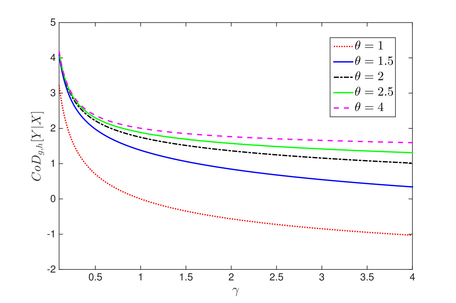 Figure 1
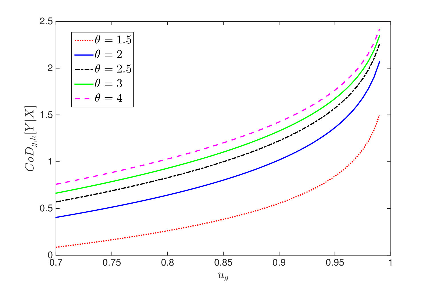 Figure 2
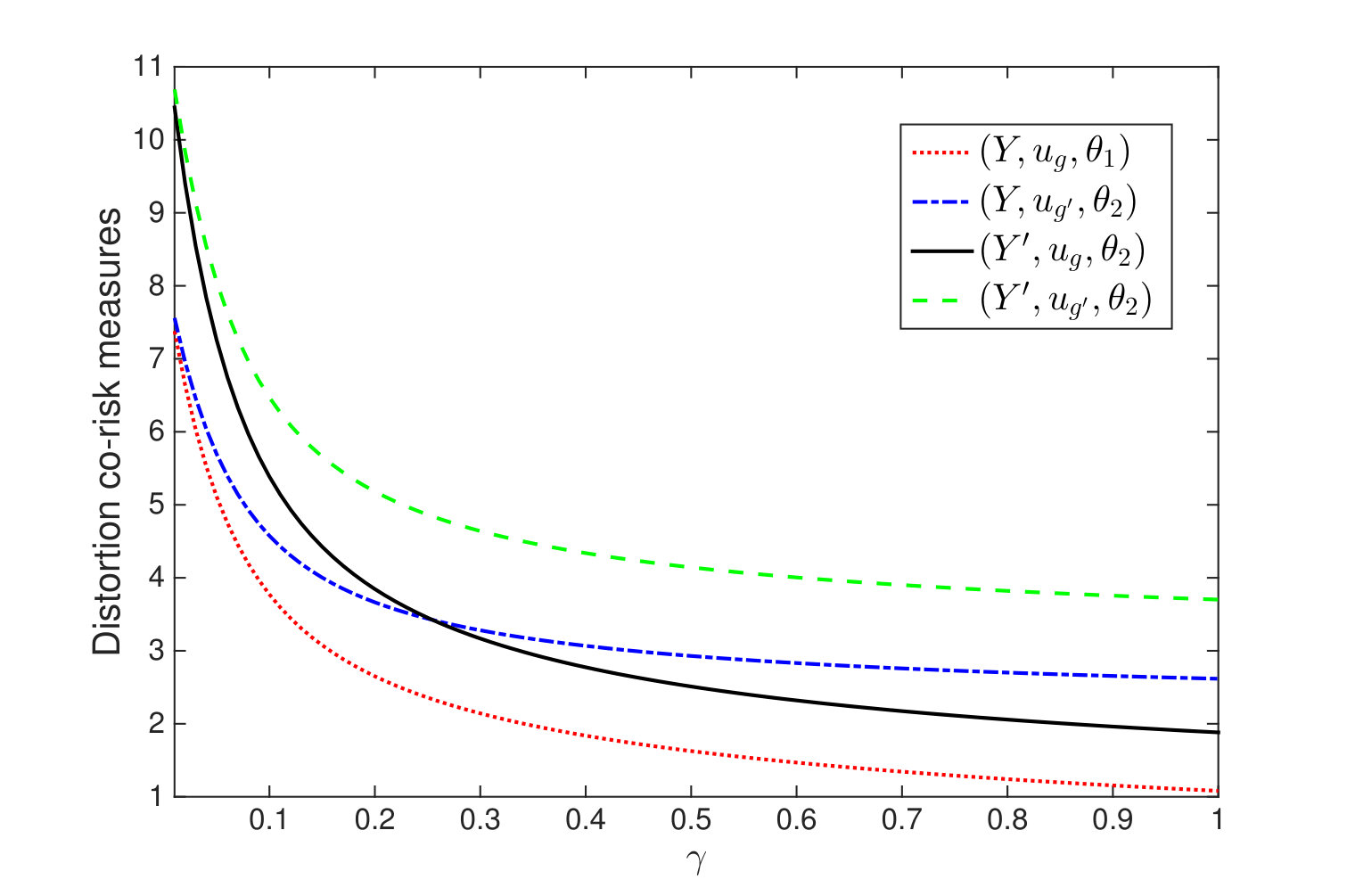 Figure 3
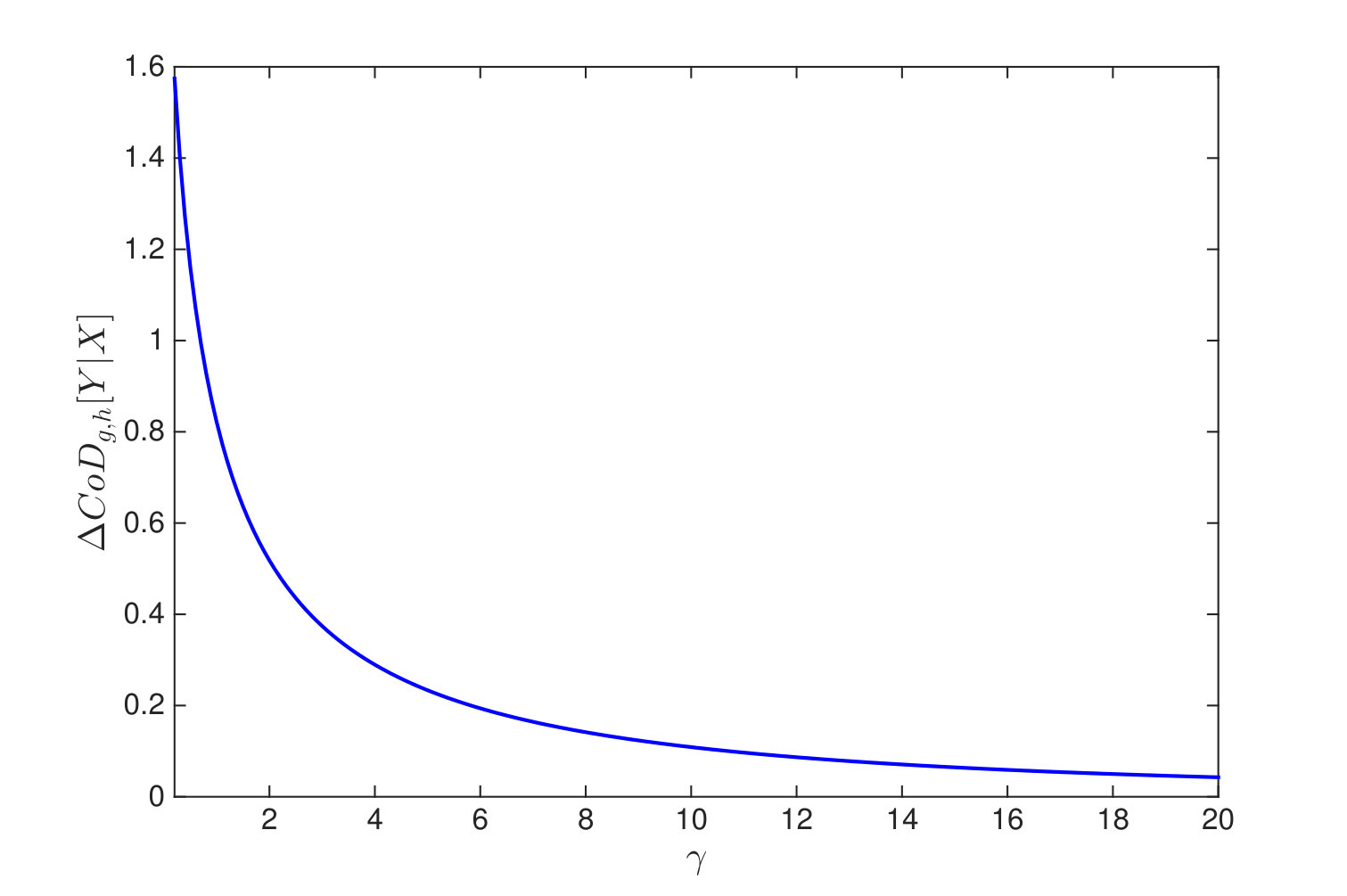 Figure 4
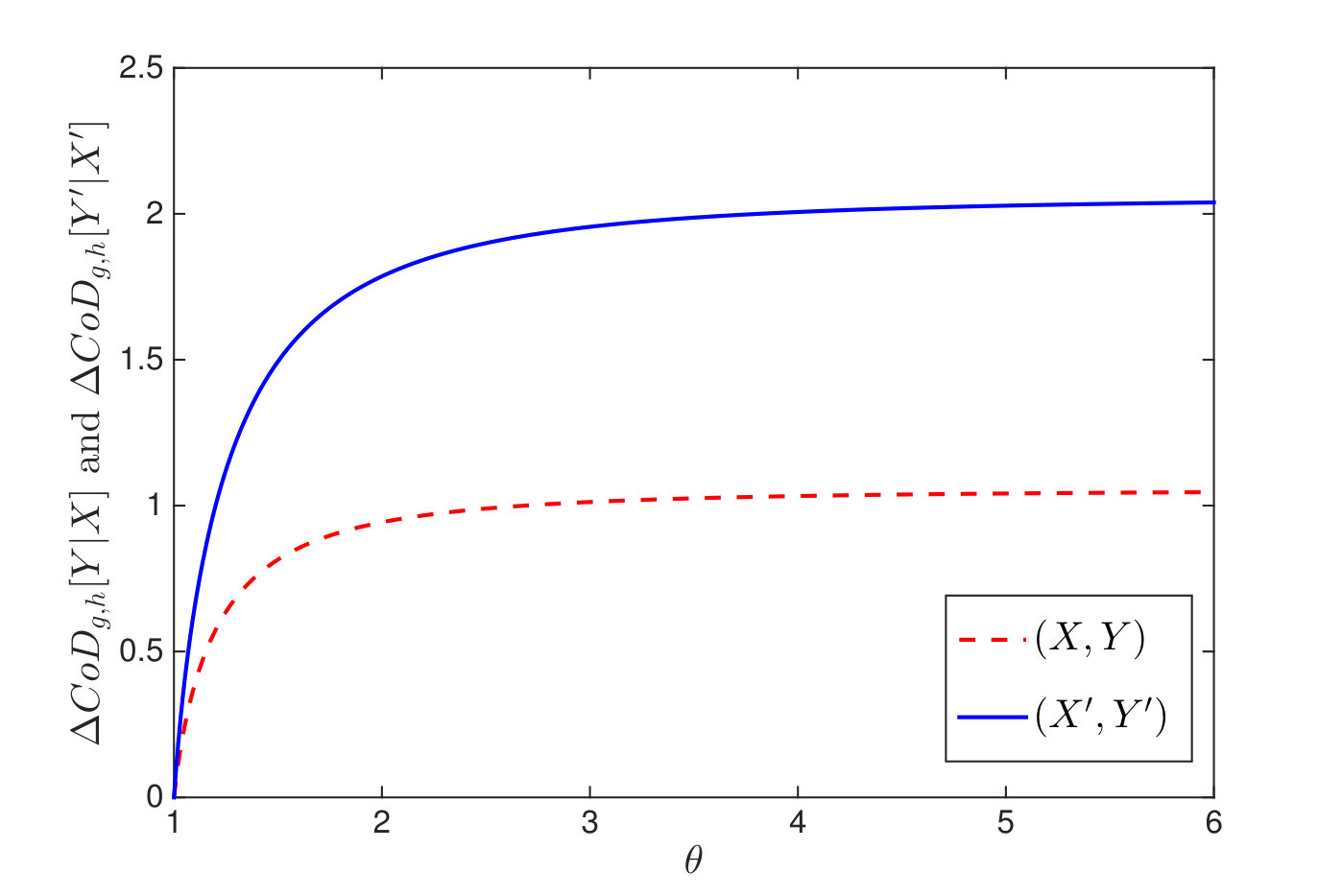 Figure 5
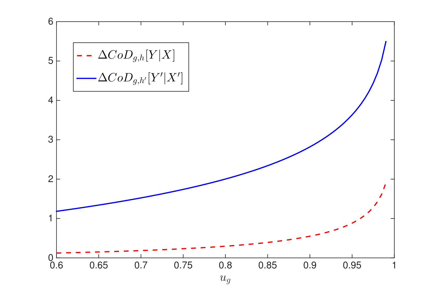 Figure 6
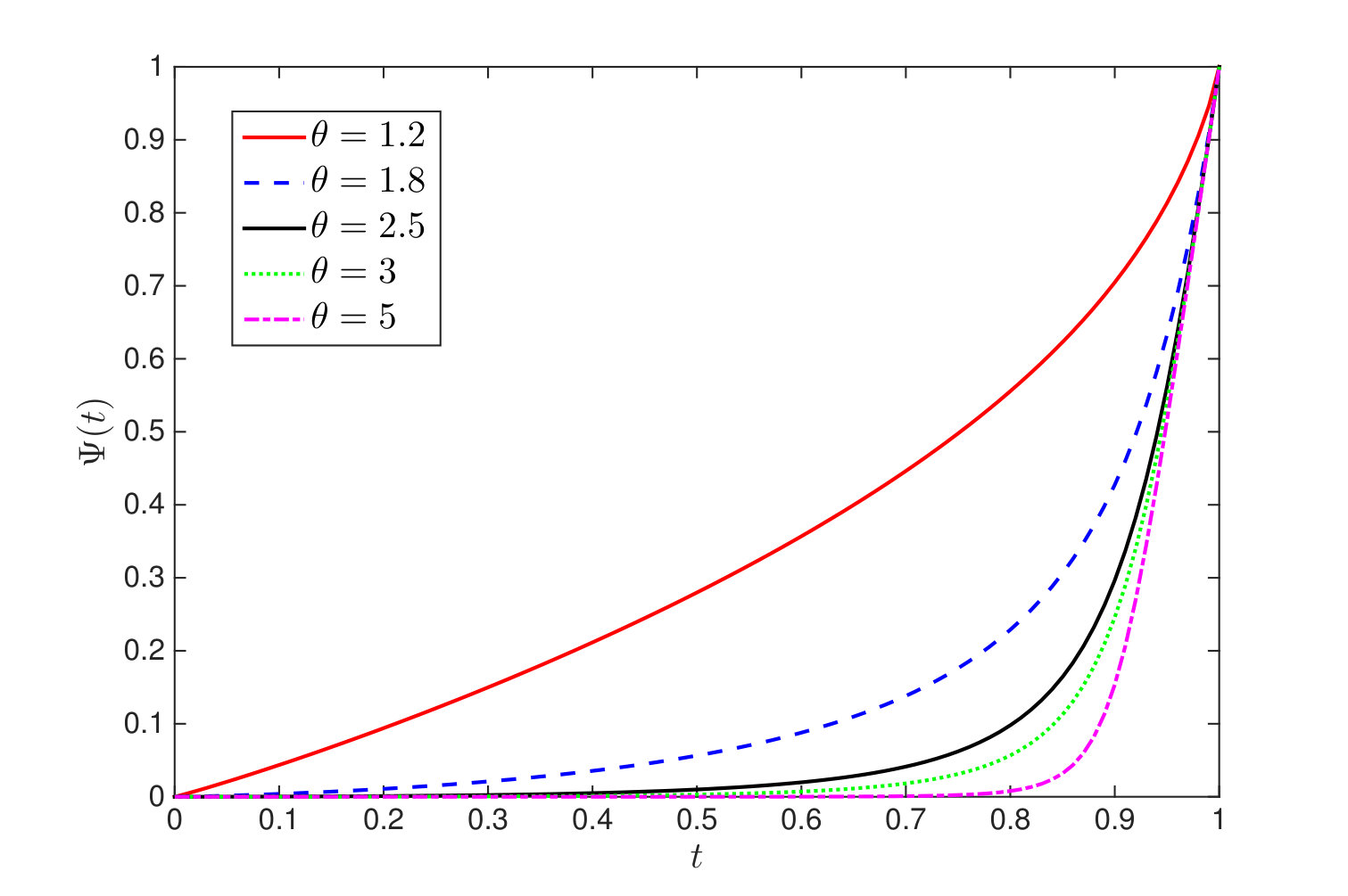 Figure 7
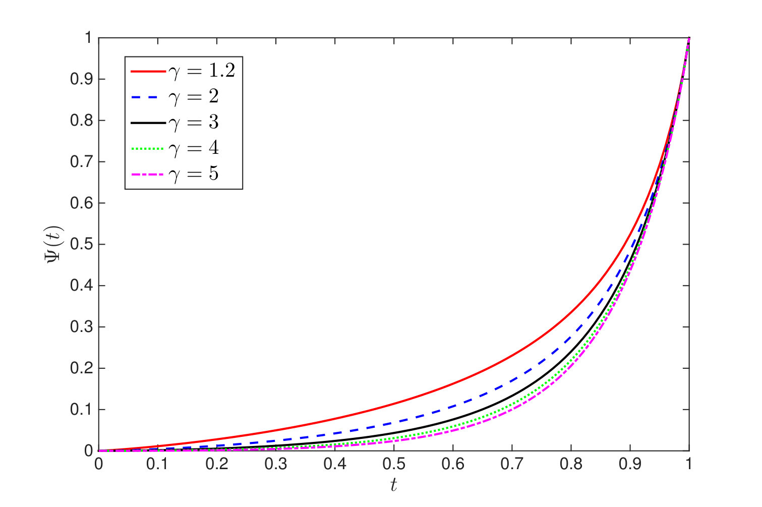 Figure 8
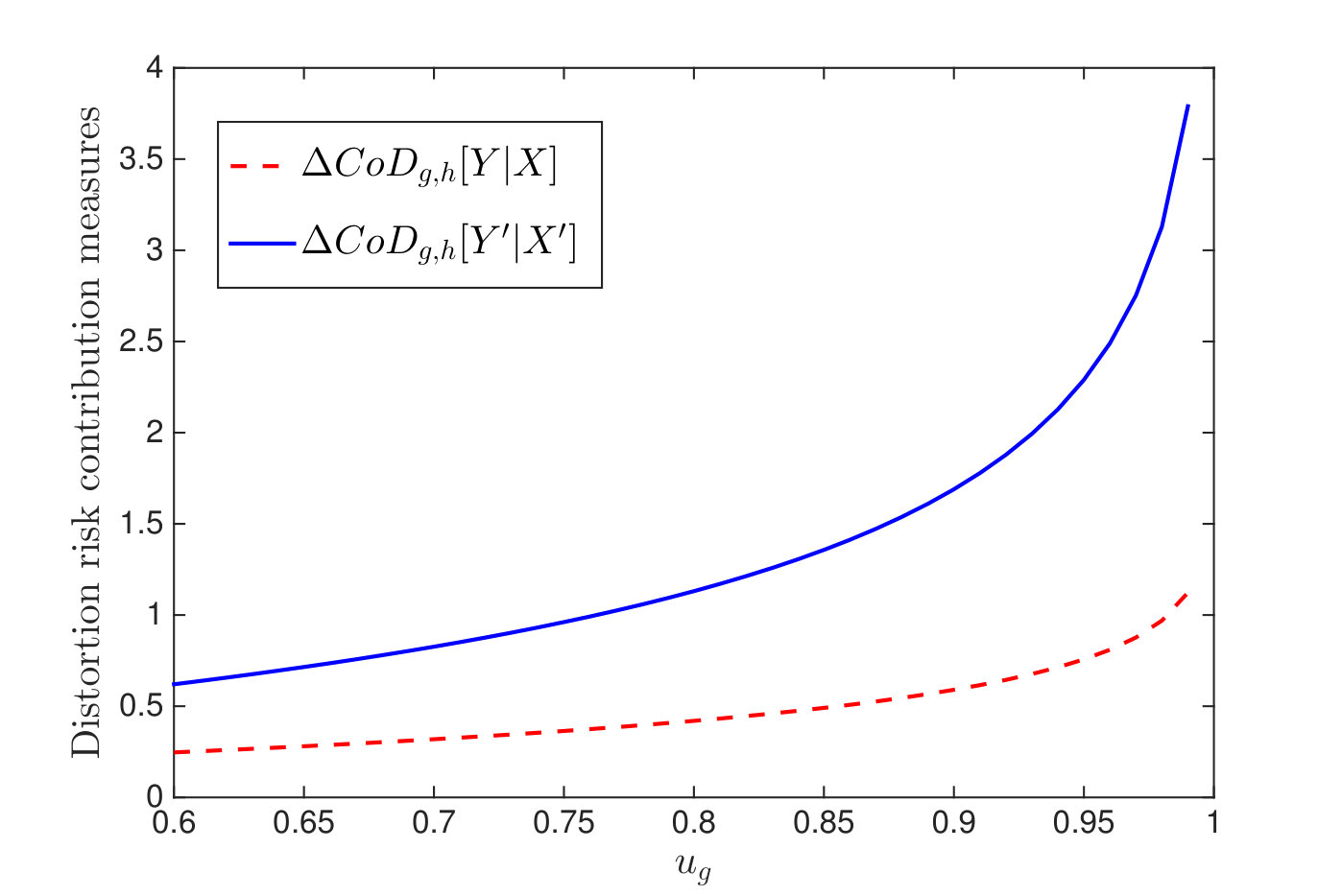 Figure 9
 Figure 10
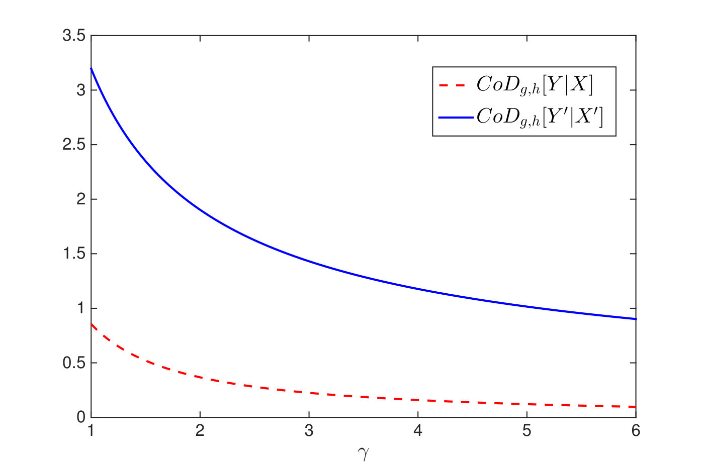 Figure 11
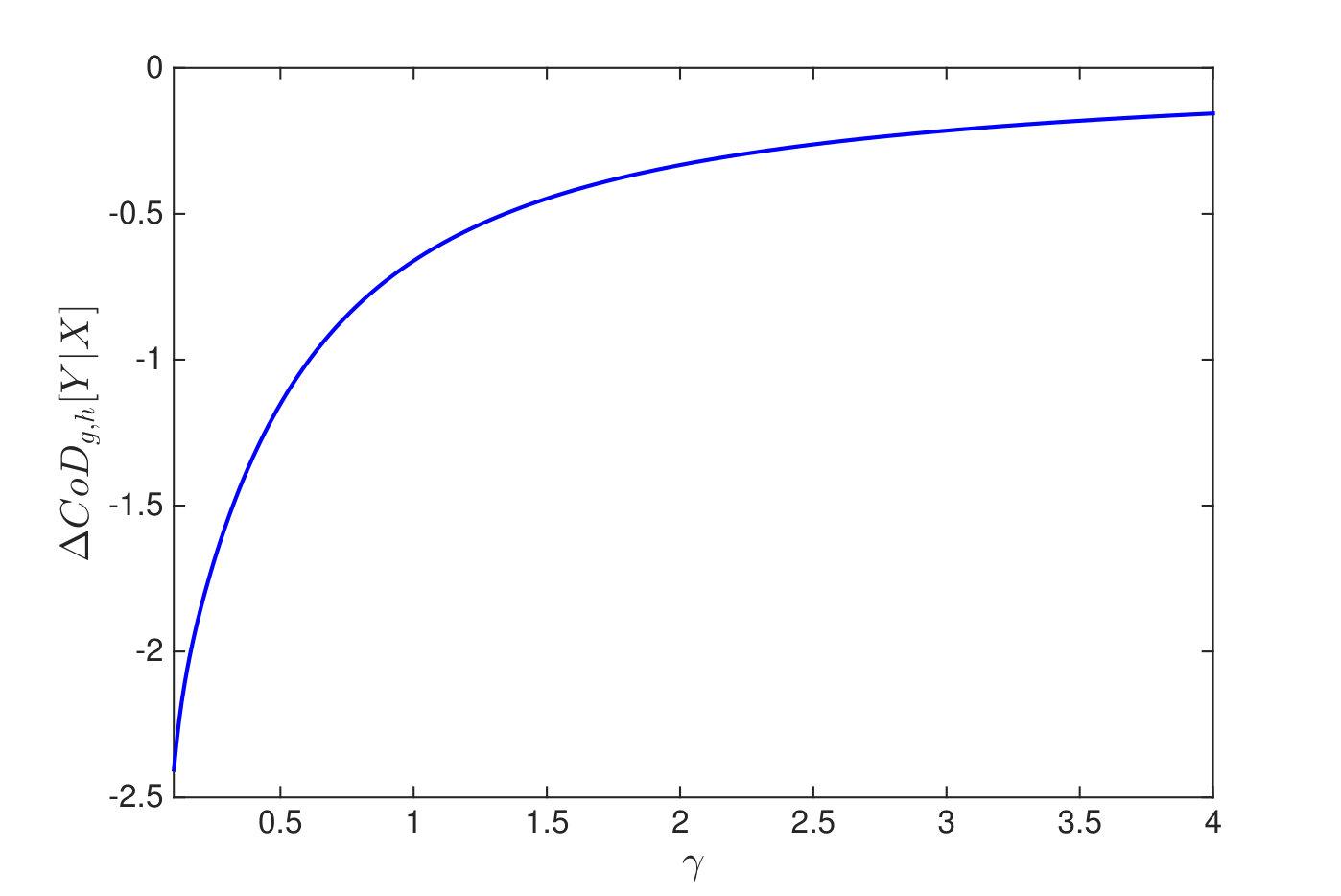 Figure 12
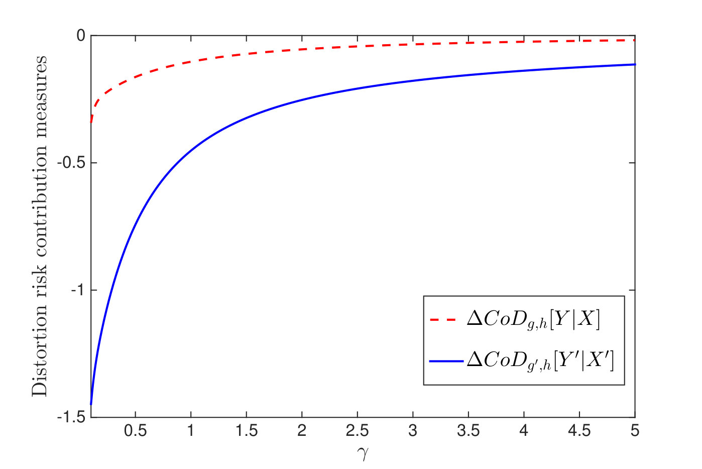 Figure 13
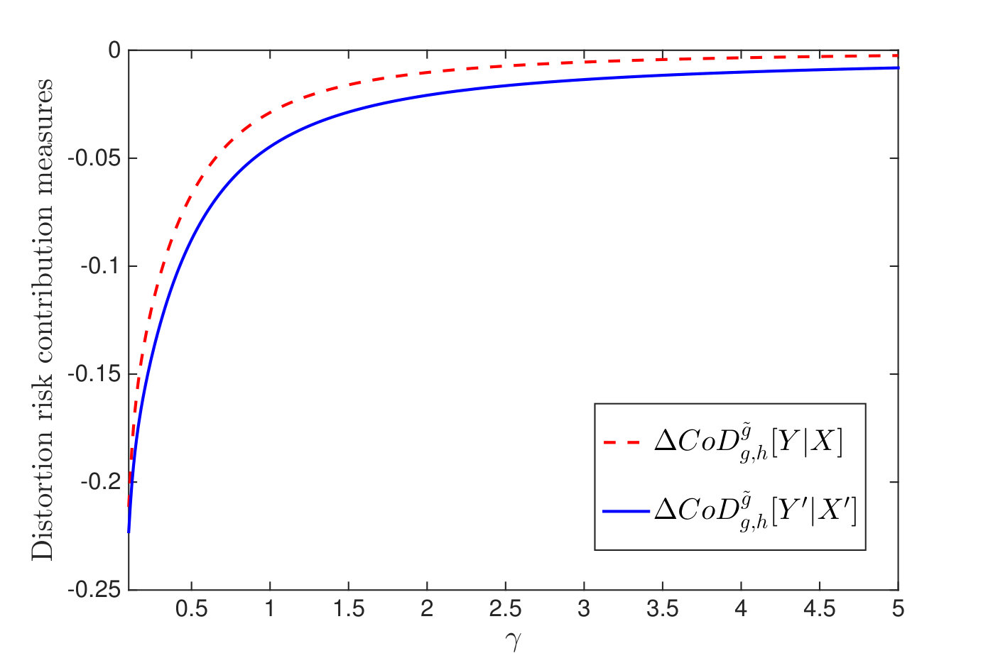 Figure 14
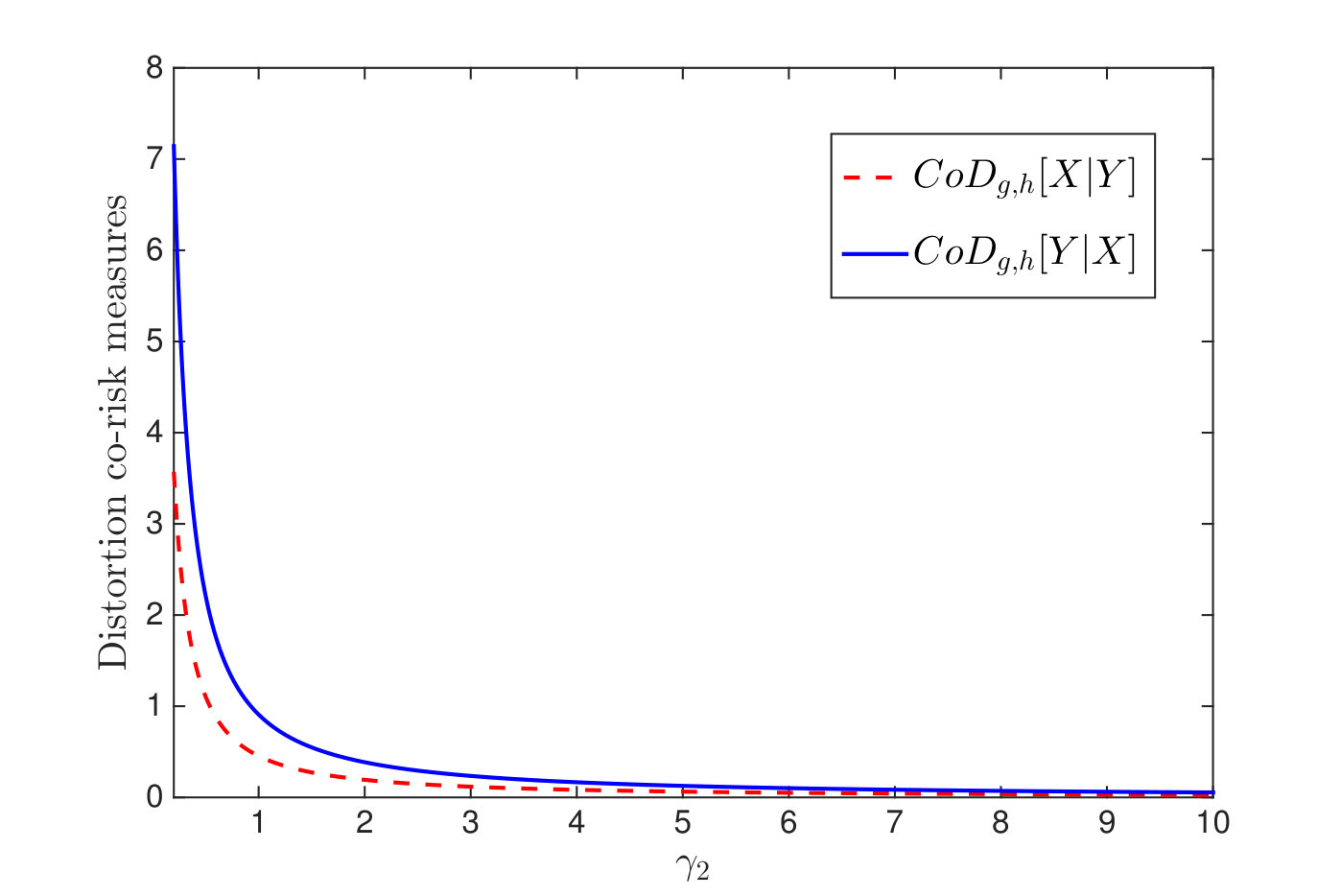 Figure 15
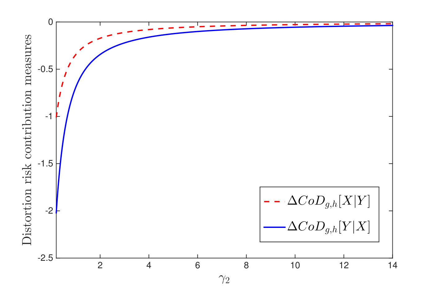 Figure 16
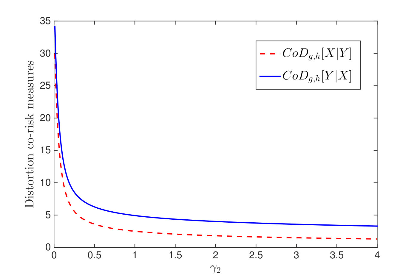 Figure 17
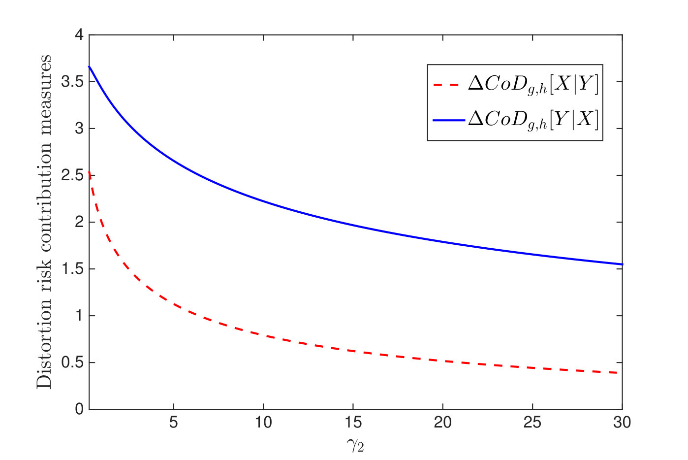 Figure 18
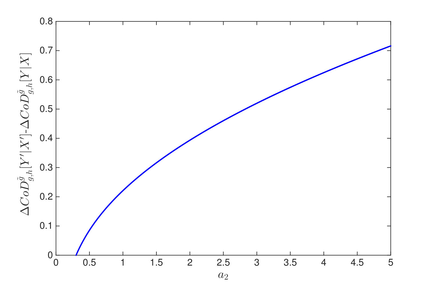 Figure 19
Peer Reviews
No public reviews on file for this paper yet. If you reviewed it on a platform where reviews are public (OpenReview, ICLR, NeurIPS, ICML), you can paste yours below so the community can read it here.
Videos
No videos yet. Explain this paper in a talk, walkthrough, or lecture? Add one.
Systemic Risk:
Conditional Distortion Risk Measures
Jan Dhaene
Faculty of Business and Economics
Katholieke Universiteit Leuven
Roger J. A. Laeven
Amsterdam School of Economics
University of Amsterdam, KU Leuven
and CentER
Yiying Zhang
School of Statistics and Data Science, LPMC and KLMDASR
Nankai University, Tianjin 300071, P. R. China
Abstract
In this paper, we introduce the rich classes of conditional distortion (CoD) risk measures and distortion risk contribution (CoD) measures as measures of systemic risk and analyze their properties and representations. The classes include the well-known conditional Value-at-Risk, conditional Expected Shortfall, and risk contribution measures in terms of the VaR and ES as special cases. Sufficient conditions are presented for two random vectors to be ordered by the proposed CoD-risk measures and distortion risk contribution measures. These conditions are expressed using the conventional stochastic dominance, increasing convex/concave, dispersive, and excess wealth orders of the marginals and canonical positive/negative stochastic dependence notions. Numerical examples are provided to illustrate our theoretical findings. This paper is the second in a triplet of papers on systemic risk by the same authors. In Dhaene et al. [2018], we introduce and analyze some new stochastic orders related to systemic risk. In a third (forthcoming) paper, we attribute systemic risk to the different participants in a given risky environment.
Keywords: Distortion risk measures; Co-risk measures; Risk contribution measures; Systemic risk; Copula; Stochastic orders.
JEL Classification: G22.
1 Introduction
Risk measures are commonly used as capital requirements, i.e., as real-valued mappings on a class of financial positions to determine the amount of risk capital to be held in reserve. The purpose of this risk capital is to make the risk given by the financial position taken by a financial institution, such as an insurance company or a bank, acceptable from a microprudential regulatory perspective. Prominent examples of risk measures are the Value-at-Risk (VaR) and the Expected Shortfall (ES).111Expected Shortfall is also referred to as Tail Value-at-Risk (TVaR) and Average Value-at-Risk (AVaR); see Definition 2.4 for the explicit definitions. Indeed, with the international adoption of financial regulatory frameworks such as the Basel Capital Accords for banks and the European Solvency Regulation for insurers, VaR has become the predominant measure of risk for financial institutions. Since its first adoption in the nineties of the previous century, an active area of research has analyzed the appealing and appalling properties of VaR (and, later, ES), and has developed new alternative theories of risk measurement. These theories build on a rich literature in actuarial mathematics and decision theory and have nowadays reached a high level of mathematical and economic sophistication.
Over the past decade we have witnessed several occurrences of pronounced transmissions of adverse economic events within a highly interconnected financial-economic network, at an international or even global scale. The interactions among risks in the form of stochastic interdependences, in part caused by dynamic feedback relations, should play a central role in quantitative risk analysis; see Denuit et al. [2005], Embrechts et al. [2005], Kaas et al. [2009], Laeven [2009], and Goovaerts et al. [2011] in the context of risk aggregation under VaR and ES. Since the 2008/09 global financial crisis, risk measures have increasingly been employed not just to provide microprudential assessments of marginal risks or aggregate portfolio risks, but also to evaluate forms of systemic risk: from a macroprudential perspective we are interested in the systemic risk that a failure or loss of one entity spreads contagiously to other entities or even to the entire financial system. Indeed, the complex system of financial institutions in a competitive economy induces an undeniable presence of interconnectedness. This interconnectedness can cause a collapse in part of the system as a result of a contagious disruption due to the failure of a singular player. Thus, the potential threat of the failure of a singular player can have a reverberating effect on the security and stability of the system and the economy as a whole. In the literature, several papers have proposed different conditional risk (co-risk) measures and risk contribution measures to evaluate the systemic risks emerging from a group of financial institutions and the interactions among them; see e.g., Gourieroux and Monfort [2013], Girardi and Ergün [2013], Adrian and Brunnermeier [2016], Brownlees and Engle [2016], Acharya et al. [2017], and the references therein.
As a simple measure of systemic risk, Adrian and Brunnermeier [2016] analyze the conditional VaR (CoVaR, see Definition 2.6). It is defined as the VaR of one specific financial institution, conditional upon the occurrence of an event that is specific to another financial institution. The prefix “Co” is meant to refer to “conditional” (or “co-movement”) and emphasizes the systemic nature of this measure of risk. In a sense, CoVaR provides a measure of a spillover effect. In related literature, Mainik and Schaanning [2014] introduce the conditional expected shortfall (CoES) and Acharya et al. [2017] propose the marginal expected shortfall (MES); see Definitions 2.7 and 2.8. For a given choice of such co-risk measures, the associated risk contribution measure evaluates how a stress scenario for one component incrementally affects another component or the entire system. Examples of risk contribution measures including CoVaR (Definition 2.9) and CoES (Definition 2.10) can be found in Girardi and Ergün [2013], Mainik and Schaanning [2014], and Adrian and Brunnermeier [2016]. Using data on U.S. financial institutions over the period 2005-2014 Kleinow et al. [2017] compare several commonly used systemic risk metrics, including CoVaR and MES. They illustrate that the alternative measurement approaches produce very different estimates of systemic risk. In particular, different systemic risk metrics may lead to contradicting assessments about the riskiness of different types of financial institutions. As mentioned in Mainik and Schaanning [2014] “… the dependence consistency or, say, dependence coherency of systemic risk indicators is a novel problem area that needs further study … questions for general characterizations or representations of functionals … are currently open.”
In the context of comparisons of these co-risk measures and risk contribution measures, an interesting paper by Sordo et al. [2018] provides sufficient conditions to stochastically order two random vectors in terms of their CoVaR, CoES, CoVaR, and CoES, where the conditions are expressed using conventional stochastic orders for the marginals under some assumptions of positive dependence. Furthermore, Fang and Li [2018] investigate how the marginal distributions and the dependence structure affect the interactions among paired risks under the above co-risk measures and risk contribution measures. It is well known that the VaR and ES arise as two special cases within the rich class of distortion risk measures [Yaari, 1987, Denuit et al., 2005, 2006, Goovaerts et al., 2010, Föllmer and Schied, 2011]. Distortion risk measures satisfy several appealing (in fact, characterizing) properties including monotonicity, translation invariance, comonotonic additivity, and positive homogeneity. Besides, distortion risk measures are consistent with the usual stochastic order (i.e., first-order stochastic dominance) under any distortion function, and with the increasing convex order (i.e., stop-loss order) under any concave distortion function. Furthermore, concave distortion risk measures occur naturally as building blocks of law-invariant convex risk measures [see Chapter 4 in Föllmer and Schied, 2011].
The aim of this paper is to introduce general and unified classes of conditional risk measures and risk contribution measures by means of distortion functions. This gives rise to conditional distortion (CoD) risk measures and distortion risk contribution (CoD) measures. We analyze the properties and present representations of these new systemic risk measures. We establish sufficient conditions for ordering two bivariate random vectors by the proposed systemic risk measures in terms of the canonical stochastic orders (e.g., first-order stochastic dominance, the increasing concave/convex order, the dispersive order, and the excess wealth order) between the marginals, dependence structure, distortion functions, and threshold quantiles. The interactions between paired risks are also investigated. Existing results in Mainik and Schaanning [2014], Sordo et al. [2018], and Fang and Li [2018] are generalized and extended.
In a somewhat related strand of the literature, Hoffmann et al. [2016] axiomatically introduced risk-consistent conditional systemic risk measures defined on multidimensional risks. This class consists of those conditional systemic risk measures that can be decomposed into a state-wise conditional aggregation and a univariate conditional risk measure. Their studies extend known results for unconditional risk measures on finite state spaces. Besides, Biagini et al. [2018] specified a general methodological framework for systemic risk measures via multidimensional acceptance sets and aggregation functions. Their approach yields systemic risk measures that can be given the interpretation of the minimal amount of cash that safeguards the aggregated system.
The organization of the present paper is as follows. In Section 2, we recall some useful definitions and concepts. In Section 3, we introduce conditional distortion (CoD) risk measures and distortion risk contribution (CoD) measures, and give some useful expressions employed in the sequel. Section 4 studies the comparisons of two random vectors under CoD-risk measures, and provides sufficient conditions for their ordering in terms of the usual stochastic order, the increasing convex order, and the increasing concave order of marginals, under appropriate assumptions on the dependence structure, distortion functions, and threshold quantiles. In Section 5, we present sufficient conditions for comparison of the distortion risk contribution measures in terms of the dispersive order and the excess wealth order of marginals. Section 6 investigates the interactions between paired risks under our proposed new CoD-risk measures and distortion risk contribution measures. Section 7 provides some numerical examples to illustrate our main findings. Section 8 concludes the paper.
2 Preliminaries
Throughout this paper, the term “increasing” is used for “non-decreasing” and “decreasing” is used for “non-increasing”. Expectations and density functions are assumed to exist when they appear. Let and be the set (space) of all univariate and bivariate distribution functions considered in the sequel. Furthermore, let be the set of real numbers and , and let be the set of strictly positive natural numbers. We use the expression ‘’ to denote that the random variable (or vector) has distribution , and use to denote the random vector .
2.1 Stochastic Orders
We denote by and two random variables (r.v.’s) with respective distribution functions (d.f.’s) and , survival functions and , and density functions and . Let and be the generalized inverses of the d.f.’s and of and , for , respectively, where by convention.
Definition 2.1**.**
* is said to be smaller than in the*
- (i)
likelihood ratio order (denoted by ) if is increasing in ;
- (ii)
hazard rate order (denoted by ) if is increasing in ;
- (iii)
usual stochastic order (denoted by ) if for all ;
- (iv)
increasing convex order (denoted by ) if for any increasing and convex function ;
- (v)
increasing concave order (denoted by ) if for any increasing and concave function ;
- (vi)
dispersive order (denoted by ) if , for all ;
- (vii)
excess wealth order (denoted by ) if , for all .
As is well known,
[TABLE]
Furthermore, the dispersive order is stronger than (i.e., implies) the excess wealth order, and is a partial order used to compare the variabilities among two probability distributions. For comprehensive discussions on these useful partial orders, we refer the reader to the monographs by Denuit et al. [2005], Marshall and Olkin [2007], and Shaked and Shanthikumar [2007].
2.2 Measuring Dependence
The following notions entail that, for a bivariate random vector, larger values of one component are associated with larger values of the other, in some specific sense.
Definition 2.2**.**
- (i)
The bivariate random vector is said to be totally positive of order 2 [reverse regular of order 2] (written as TP2* [RR2]) if , for all , and , for all .*
- (ii)
* is said to be stochastically increasing [decreasing] in (written as ) if , for all .*
- (iii)
The bivariate random vector is said to be positively [negatively] dependent through stochastic ordering (PDS [NDS]) if and .
- (iv)
* is said to be right tail increasing [decreasing] in (written as ) if is increasing in , for all .*
- (v)
The bivariate random vector is said to be positive [negative] quadrant dependent (PQD [NQD]) if, for all , it holds that
[TABLE]
or equivalently,
[TABLE]
The following implications (with slight abuse of notation) are well known:
[TABLE]
[TABLE]
It is also clear that if is TP2 [RR2] then it must be PDS [NDS]. Besides, is TP2 [RR2] if and only if its copula is TP2 [RR2] [see Müller and Stoyan, 2002, Cai and Wei, 2012]. For more detailed discussions, interested readers are referred to Barlow and Proschan [1975], Block et al. [1982], Joe [1997], and Denuit et al. [2005].
2.3 Comparing Dependence and Copulas
Consider a bivariate random vector with respective marginal d.f.’s and and joint d.f. . It is well known that any such bivariate d.f. admits the decomposition
[TABLE]
where is a bivariate d.f. on with uniform margins [Sklar, 1959], i.e., there exist r.v.’s such that . The function is called a copula of . If both and are continuous, then is uniquely determined by . The copula characterizes the dependence of the random vector . We also denote by the joint tail function for two uniform r.v.’s whose joint d.f. is the copula , that is,
[TABLE]
The joint tail function should not be confused with the survival copula of and , which is defined as
[TABLE]
The survival copula couples the joint survival function to its univariate margins (survival functions) in a manner completely analogous to how a copula links the joint d.f. to its margins. Clearly, .
We next recall the definition of the concordance order [see Definition 2.8.1 in Nelsen, 2007].
Definition 2.3**.**
Given two copulas and , is said to be smaller than in concordance order (denoted as ) if , for all .
The concordance order is also referred to as the correlation order or the positive quadrant dependence (PQD) order in the literature [see Dhaene and Goovaerts, 1996, 1997, Nelsen, 2007]. It is a partial order as not every pair of copulas is concordance-comparable. Besides, the canonical scale-free dependence measures given by Kendall’s tau and Spearman’s rho are well known to be increasing with respect to the concordance order.
2.4 Distortion Risk Measures
We state the following definition:
Definition 2.4**.**
The VaR and ES of a r.v. with d.f. at confidence level are defined as
[TABLE]
and
[TABLE]
provided that the integral exists.
VaR and ES occur as special cases of distortion risk measures [Yaari, 1987, Denuit et al., 2005, 2006, Dhaene et al., 2006, Goovaerts et al., 2010, Föllmer and Schied, 2011]. In full generality, a distortion function is an increasing function such that and . The set of all distortion functions is denoted by . A distortion risk measure, then, is a functional mapping the elements of to the real line, as follows:
Definition 2.5**.**
For a distortion function , the distortion risk measure of a r.v. with d.f. is defined as
[TABLE]
In particular, if is a nonnegative r.v., then
[TABLE]
It is well known that distortion risk measures enjoy, and can be characterized by, the properties of monotonicity, translation invariance, comonotonic additivity, and positive homogeneity. Besides, distortion risk measures are consistent with the usual stochastic order under any distortion function , and with the increasing convex order under any concave distortion function. Wirch and Hardy [2001] showed that a distortion risk measure is coherent, i.e., monotonic, translation invariant, positively homogeneous, and subadditive [see e.g., Föllmer and Schied, 2011, Laeven and Stadje, 2013] if and only if the distortion function is concave. Furthermore, concave distortion functions are the building blocks of law-invariant convex risk measures [see Chapter 4 in Föllmer and Schied, 2011].
The two prominent examples of distortion risk measures given by and correspond to the distortion functions and , for , respectively. Obviously, the distortion function for VaR is not continuous but left-continuous, while the distortion function for ES is continuous and concave but not differentiable everywhere. Besides, the incomplete beta function, the Wang distortion or Esscher-Girsanov transform, and the lookback distortion are commonly used special cases of distortion functions; see Denuit et al. [2006] and Goovaerts and Laeven [2008]. It is easily verified [see e.g., Belles-Sampera et al., 2014] that for a r.v. and any two distortion functions , implies that .
Next, we introduce the notion of a dual distortion function. Consider a distortion function and define the related function by , for . Obviously, is also a distortion function, called the dual distortion function of . It is well known that, for any r.v. and distortion function , and [see Lemma 5 in Dhaene et al., 2012]. Note that if is left-continuous, then is right-continuous (c.f. Theorems 4 and 6 in Dhaene et al. [2012]).
For a right-continuous distortion function , the transformation of the tail function of given by defines a new tail function associated to a r.v. , which is the distorted counterpart of the r.v. , induced by distorting with distortion function .
For more discussions on the properties and applications of distortion risk measures, one may refer to Wang et al. [1997], Hürlimann [2004], Denuit et al. [2005, 2006], Dhaene et al. [2006], Balbás et al. [2009], and Dhaene et al. [2012].
2.5 Co-Risk Measures and Risk Contribution Measures
Conditional risk (co-risk) measures are increasingly employed as measures of systemic risk. Prototypical examples of co-risk measures include the conditional Value-at-Risk (CoVaR) [Adrian and Brunnermeier, 2016, Girardi and Ergün, 2013], the conditional Expected Shortfall (CoES) [Mainik and Schaanning, 2014], and the marginal Expected Shortfall (MES) [Acharya et al., 2017]. For a given co-risk measure, the corresponding risk contribution measure assesses the incremental effect of a stress scenario. Well known examples of risk contribution measures include CoVaR and CoES; see Girardi and Ergün [2013], Mainik and Schaanning [2014], and Adrian and Brunnermeier [2016].
The definition of CoVaR is given as follows:
Definition 2.6**.**
Let . Then,
[TABLE]
The above definition is adapted by Mainik and Schaanning [2014] to the case of CoES, under which the coherence of ES is inherited by CoES:
Definition 2.7**.**
Let . Then,
[TABLE]
One easily verifies that, with continuous marginals, the CoES can be represented through a conditional expectation of , in a manner similar to the familiar representation of ES:
[TABLE]
The definition of MES is given as follows:
Definition 2.8**.**
Let . Then,
[TABLE]
To measure the risk contribution of to , one may compare , which is the VaR of conditional upon being in a stress scenario, to , which evaluates unconditionally. Alternatively, one may replace the benchmark by the conditional VaR of given that exceeds its median [see Mainik and Schaanning, 2014, Adrian and Brunnermeier, 2016].
Definition 2.9**.**
Let . Then,
[TABLE]
Risk contribution measures can, of course, also be defined by invoking e.g., CoES, as follows [see Acharya et al., 2017, Karimalis and Nomikos, 2018]:
Definition 2.10**.**
Let . Then,
[TABLE]
3 Conditional Distortion Risk Measures and Distortion Risk Contribution Measures
Consider a bivariate random vector with marginal d.f.’s and joint d.f. . We define the conditional distortion (CoD) risk measure as a mapping from a bivariate distribution to the real line. Specifically, the CoD-risk measure is defined as follows.
Definition 3.1**.**
For ,
[TABLE]
where is presented in Definition 2.5.
Remark 3.2**.**
- (a)
Note that in Definition 3.1 and are distortion functions imposed on the d.f.’s of and , respectively.
- (b)
Obviously, the CoD-risk measure presented in Definition 3.1 contains the CoVaR and CoES as special cases. More explicitly, we have
- (i)
if and , then ;
- (ii)
if and , then .
- (iii)
if and , then .
Besides, the CoD-risk measure provides two other related types of conditional risk measures:
- (iv)
if and , then ;
- (v)
if and , then
[TABLE]
which was defined in Equation (10) of Boyle and Kim [2012]**.
- (c)
The CoD-risk measure does not in general satisfy the subadditivity property; for example, if , it reduces to the VaR, which is not subadditive in general. However, if is concave then the CoD-risk measure inherits the subadditivity property of .
- (d)
It should be noted that we can replace by any real value to generalize Definition 3.1. However, all of the existing methods concerned with VaR, median, and ES can be treated as special cases of distortion risk measures under appropriate conditions.
To illustrate the generality of CoD-risk measures, the following example provides an illustration of the class of CoD-risk measures that goes beyond the existing conditional risk measures such as CoVaR, CoES, and MES that are present in the current literature.
Example 3.3**.**
Assume that is a nonnegative r.v. and consider the distortion function , for and . Let be independent copies of the conditional r.v. , for . According to Definition 3.1, we then have
[TABLE]
where is the maximum order statistic of . This means that the CoD-risk measure can be represented as the expectation of the maximum order statistic computed from a set of i.i.d. r.v.’s with d.f. .
For a given CoD-risk measure, we can define the associated distortion risk contribution (CoD) measure, as follows.
Definition 3.4**.**
For ,
[TABLE]
where
[TABLE]
Remark 3.5**.**
The distortion risk contribution measure defined in Definition 3.4 contains and as special cases. Indeed,
- (i)
if and , then ;
- (ii)
if and , then .
Furthermore, the distortion risk contribution measure also provides two related contribution measures which are absent in the existing literature:
- (iii)
if and , then
[TABLE]
- (iv)
if and , then
[TABLE]
It should be mentioned that Boyle and Kim [2012] defined one type of risk contribution measure (see their Equation (8)) as
[TABLE]
for which the conditional event is based on but not .
The following example provides the expression of the distortion risk contribution measure of Definition 3.4, under the setup of Example 3.3.
Example 3.6**.**
Under the setup of Example 3.3, we have
[TABLE]
where is the maximum order statistic of with being independent copies of , for .
We can also define risk contribution measures with respect to different distortion functions for the risk , henceforth sometimes referred to as distortion risk contribution measures of Type-II to distinguish them from the distortion risk contribution measures of Type-I in Definition 3.4:
Definition 3.7**.**
For ,
[TABLE]
Remark 3.8**.**
It is worth noting that the distortion risk contribution measure of Definition 3.7 contains and as special cases. More explicitly,
- (i)
if , , and , then ;
- (ii)
if , , and , then .
The next example provides an illustration of the distortion risk contribution measures arising from Definition 3.7.
Example 3.9**.**
Under the setup of Example 3.3, let be independent copies of the conditional r.v. , for . Then,
[TABLE]
where and are the maximum order statistics of and , respectively.
In the next theorems, we present some useful expressions and properties of our three types of CoD-risk measures and distortion risk contribution measures introduced in Definitions 3.1, 3.4, and 3.7.
Theorem 3.10**.**
Let where is a copula of . If is continuous and strictly increasing, and is left-continuous, then
[TABLE]
where , for , and for .
Proof.
Since is continuous and strictly increasing, , and the marginals of are uniform, it follows that . Then, the d.f. of can be written as
[TABLE]
which in turn implies that by using the argument that the event is equivalent to , for any . Hence, by applying Fubini’s theorem and a change of variable [see Theorem 6 in Dhaene et al., 2012] one can verify that
[TABLE]
Thus, the proof is established.
Remark 3.11**.**
Consider the setup of Theorem 3.10. Define the generalized upper inverses and with by convention. Since the event is equivalent to , we have , for . If now, under the setup of Theorem 3.10, were right-continuous instead of left-continuous, then, by applying Theorem 4 in Dhaene et al. [2012], expression (1) can be modified as
[TABLE]
Note that . If is continuous and strictly increasing, and is continuous and strictly increasing in for any (which implies that is continuous and strictly increasing), we have and , which implies that the distortion function in Theorem 3.10 can be either left-continuous or right-continuous (given that is continuous and strictly increasing). Then, by applying Theorem 7 of Dhaene et al. [2012], can be also assumed to be any general distortion function, i.e., a convex combination of left-continuous and right-continuous distortion functions.
Corollary 3.12**.**
Under the setup of Theorem 3.10,
- (i)
if and , then
[TABLE]
which is defined in Girardi and Ergün [2013]**;
- (ii)
if and , then
[TABLE]
which is defined in Mainik and Schaanning [2014]**.
Based on Theorem 3.10, we have the following result.
Theorem 3.13**.**
Let where is a copula of . If is continuous and strictly increasing, and is left-continuous, then
[TABLE]
[TABLE]
where , , for , and for .
4 Stochastic Orders and CoD-Risk Measures
In the sequel, we always assume that the d.f.’s of and are continuous and strictly increasing and that the distortion functions for and are left-continuous, to avoid unnecessary technical discussions. We note that, if the d.f.’s of and are continuous and strictly increasing and both and are continuous and strictly increasing in for any , then, in light of Remark 3.11, all of our results can be generalized to the case when the distortion functions for and are right-continuous or general, that is, a convex combination of left-continuous and right-continuous distortion functions [see Theorem 7 of Dhaene et al., 2012].
4.1 The Risks and Have the Same Distribution
This subsection considers sufficient conditions for the CoD-risk measures of two bivariate random vectors and to be ordered, where and have common d.f.’s. The next theorem states that the CoD-risk measure preserves the ordering induced by “” between the copulas and by the distortion functions applied to and .
Theorem 4.1**.**
Let and be two bivariate random vectors having the same marginals but different copulas and , respectively. Then, and imply that .
Proof.
Let and . From Theorem 3.10, we have
[TABLE]
where for .
We first show that . Since is increasing, this reduces to showing that , i.e., for . Thus, it suffices to show that for , that is,
[TABLE]
which is in fact guaranteed by the condition .
On the other hand, we can verify that , and because of for . Then, by using integration by parts, one has
[TABLE]
which yields that . Hence, the proof is established.
The following result, not necessarily requiring , can be easily derived from Theorem 4.1 when is the distortion function of VaR.
Corollary 4.2**.**
Let and be two bivariate random vectors having copulas and , respectively. Suppose that and , for some . Then, and imply that .
Remark 4.3**.**
Theorem 4.1 and Corollary 4.2 do not hold in general if and adopt different distortion functions, i.e., if .
Remark 4.4**.**
Under the additional assumption that , the result of Corollary 4.2 reduces to Theorem 3.4 of Mainik and Schaanning [2014].
To conclude this subsection, we investigate the effects of threshold quantiles of and and the dependence structure among on the CoD-risk measures.
Theorem 4.5**.**
Let and be two bivariate random vectors having copulas and , respectively. Suppose that and . Let and . Then if , and either one of the following two conditions holds:
- (i)
* and or or both hold;*
- (ii)
* and or or both hold.*
Proof.
We only give the proof for (i). The proof for (ii) can be established in a similar manner. We assume that and (the other two cases follow similarly). Let and . In light of Theorem 3.10, we have
[TABLE]
By making use of a change of variable , we obtain
[TABLE]
where . Similarly, by letting and , we have
[TABLE]
where . Since , , and , we have
[TABLE]
In order to show the nonnegativity of (4), it suffices to show that , for all . Since , one has , for all . Thus, it is enough to show that , for all , that is,
[TABLE]
Taking into account that , we have that
[TABLE]
Thus, by using (6), (5) can be established if we can show that
[TABLE]
Since and , it holds that
[TABLE]
which proves (7) and thus the desired result is obtained.
Theorem 4.5 states that, if and are positively [negatively] dependent through , then a larger distortion function employed for risk , more concordance of the copula, together with a larger [smaller] threshold quantile adopted for risk lead to a larger CoD-risk measure.
Remark 4.6**.**
Let be a bivariate random vector having copula . Suppose that and . Then, in light of Theorem 4.5(ii), we have . This means that if is negatively dependent of through RTD, then a larger distortion function for and a smaller distortion function for lead to a larger value of the CoD-risk measure.
Remark 4.7**.**
Let and be two bivariate random vectors having the same copula . Suppose that , and either (i) and or or both hold, or (ii) and or or both hold. Then Theorem 4.5 implies that for all . This result states that is more relevant for than if is positively [negatively] dependent of (and/or ) through RTI [RTD] and the threshold quantile of is smaller [larger] than that of , which is consistent with the systemic relevance order proposed in Definition 12 of Dhaene et al. [2018].
4.2 The Risks and Have Different Distributions
In this subsection, we present sufficient conditions on the dependence structure and distortion functions for the CoD-risk measures of two bivariate random vectors and to be ordered when and have different d.f.’s.
Sordo and Ramos [2007] provided a useful characterization of the usual stochastic order and the increasing convex order as follows. In a similar manner, we can give an equivalent characterization of the increasing concave order.
Lemma 4.8**.**
Let and be two r.v.’s with d.f.’s and , respectively. Then, if and only if
[TABLE]
for all increasing [increasing convex, increasing concave] .
Proof.
The proof for the usual stochastic order and the increasing convex order can be found in Sordo and Ramos [2007]. We only prove the characterization of the increasing concave order.
Assume that . According to Theorem 4.A.1 in Shaked and Shanthikumar [2007], we know that is equivalent to . Then, by using the equivalent characterization of the increasing convex order, it follows that
[TABLE]
for all increasing convex . Note that
[TABLE]
Hence, we have
[TABLE]
that is
[TABLE]
where is increasing and concave on . Hence, the proof is established.
Next, for two given random vectors and , we present sufficient conditions in terms of stochastic orders of the marginal d.f.’s of and , the respective copulas and dependence structure, and the distortion functions for their CoD-risk measures to be ordered.
Theorem 4.9**.**
Let and be two bivariate random vectors having copulas and , respectively. Suppose that , , and .
- (i)
Suppose that or or both hold. Then, implies that for any and increasing [increasing concave] .
- (ii)
Suppose that or or both hold. Then, implies that for any and increasing convex .
Proof.
We only give the proof for the increasing convex ordering between and . The proofs for the usual stochastic ordering and the increasing concave ordering can be obtained in a similar manner by using Lemma 4.8. Furthermore, we only consider the case of since the proof can be carried out similarly for .
Let and . In light of Theorem 3.10, we have
[TABLE]
By making use of a change of variable , we obtain
[TABLE]
where . Note that is increasing and convex in since is nonnegative and increasing in because . On the other hand, it is easy to verify that is also increasing convex due to the increasing concavity of . Hence, we know is increasing and convex in . Similarly, by we can obtain
[TABLE]
where . The desired result boils down to showing that
[TABLE]
On the one hand, by using Lemma 4.8, implies that
[TABLE]
On the other hand, implies that , and thus since . Because and , we then have
[TABLE]
which means that
[TABLE]
Upon combining (10) and (11), the desired result (9) is established.
Remark 4.10**.**
Definition 2 of Dhaene et al. [2018] defines the systemic contribution order in terms of the increasing convex order. More explicitly, consider the market of losses , the corresponding microprudential regulation , and the aggregate residual loss level . Individual loss is said to be “smaller in systemic contribution order” (denoted by ) than individual loss under microprudential regulation and aggregate loss level , if
[TABLE]
According to Theorem 4.9(i), if , , , , , and or or both hold, then implies that
[TABLE]
for all concave , which is consistent with the definition when taking .
The following result, not necessarily requiring , can be derived from Theorem 4.9 when corresponds to the distortion function of VaR.
Corollary 4.11**.**
Let and be two bivariate random vectors having copulas and , respectively. Suppose that , , and .
- (i)
Suppose that or or both hold. Then, implies that for any increasing [increasing concave] .
- (ii)
Suppose that or or both hold. Then, implies that for any increasing convex .
Remark 4.12**.**
In the special case that , the result of Corollary 4.11(i) reduces to Theorem 12 in Sordo et al. [2018].
The next result generalizes Theorem 4.9 to the case of different d.f.’s of and , where we can replace the condition ‘’ by requiring that .
Theorem 4.13**.**
Let and be two bivariate random vectors having copulas and , respectively. Suppose that , , and , where and .
- (i)
Suppose that or or both are PDS. Then, implies that for any increasing [increasing concave] .
- (ii)
Suppose that or or both are NDS. Then, implies that for any increasing convex .
Proof.
Note that if is PDS [NDS], then and . The proof is then easily obtained by combining the proof methods in Theorems 4.5 and 4.9.
5 Stochastic Orders and Distortion Risk Contribution Measures
Consider two bivariate random vectors and . This section provides sufficient conditions in terms of stochastic orders of the marginal d.f.’s of and , the respective copulas and dependence structure, and the distortion functions for their distortion risk contribution measures to be ordered.
5.1 Dispersive Order and Distortion Risk Contribution Measures
The following lemma, adapted from Sordo et al. [2018], is helpful to establish our main results linking the dispersive order between marginals with distortion risk contribution measures.
Lemma 5.1**.**
Let and be two continuous r.v.’s with d.f.’s and , respectively. Let be a convex distortion function and let be another right-continuous distortion function such that , for all . Denote by [] the distorted r.v.’s induced from [] by the distortion functions []. If , then
- (i)
, for ;
- (ii)
, for .
Proof.
The proof can be obtained by using similar arguments as in Lemma 14 in Sordo et al. [2018], and thus is omitted here for brevity.
5.1.1 Type-I Distortion Risk Contribution Measures:
We first study the sufficient conditions for .
Theorem 5.2**.**
Let and be two bivariate random vectors having copulas and , respectively. Suppose that and .
- (i)
If , and or or both hold, then for any .
- (ii)
If , and or or both hold, then for any .
Proof.
We only give the proof of (i) since the proof of (ii) is similar by applying Lemma 5.1(i). Suppose that . According to Theorem 3.13 and the proof of Theorem 3.10, we have
[TABLE]
where and are the distorted r.v.’s induced from and by the concave distortion functions
[TABLE]
Since , it clearly holds that for all . From and Lemma 14 in Sordo et al. [2018], we have
[TABLE]
which yields the desired result since is increasing in .
The next theorem generalizes Theorem 5.2 to the case where and may have different d.f.’s.
Theorem 5.3**.**
Let and be two bivariate random vectors having copulas and , respectively. Let and . Suppose that .
- (i)
If is PDS, , and , then for any .
- (ii)
If is NDS, , and , then for any .
The following result is partially taken from Theorem 5 in Sordo et al. [2015] and the proof for the case of a convex distortion function can be established using similar arguments as in the proof of Theorem 5 in Sordo et al. [2015].
Lemma 5.4**.**
Let be a r.v. and let be a concave [convex] distortion function. Then , where is the distorted r.v. induced from by applying the distortion function .
Recall that a (nonnegative) r.v. has an increasing [decreasing] failure rate (IFR [DFR]) if, and only if, its survival function is log-concave [log-convex].
Theorem 5.5**.**
Let be a bivariate random vector with copula . Assume that is DFR. Then for any if either one of the following two conditions holds:
- (i)
* and ;*
- (ii)
* and .*
Proof.
We only give the proof for (i) since the proof can be established in a similar manner for (ii). According to Theorem 3.13 and the proof of Theorem 3.10, we have
[TABLE]
where is a distorted r.v. induced from by the concave distortion function
[TABLE]
Then, from Lemma 5.4, we have . Since is DFR, it follows that upon invoking Theorem 3.B.20(a) of Shaked and Shanthikumar [2007]. Therefore, it holds that
[TABLE]
which implies that is increasing in . Since and , we then have that
[TABLE]
which yields the desired result.
Remark 5.6**.**
If , is DFR, , , and such that , then Theorem 5.5 reduces to the result of Theorem 17 in Sordo et al. [2018].
Upon combining Theorems 5.2 and 5.5, the following result can be obtained immediately, which generalizes the result of Corollary 19 in Sordo et al. [2018].
Corollary 5.7**.**
Let and be two bivariate random vectors having copulas and , respectively. Suppose that , or or both hold, and or or both are DFR. Then, , , and imply that for any .
The following result generalizes the above result to the case of risks and having different d.f.’s.
Theorem 5.8**.**
Let and be two bivariate random vectors having copulas and , respectively. Let and . Suppose that or or both are PDS, and or or both are DFR. Then, , , , and imply that for any .
Proof.
By using the proof method in Theorem 4.13, the result can be obtained from Theorem 5.3.
5.1.2 Type-II Distortion Risk Contribution Measures:
In this subsection, we turn our attention to studying how the dependence structure, threshold quantile of , and the stochastic ordering according to which varies change the value of the distortion risk contribution measure .
Theorem 5.9**.**
Let and be two bivariate random vectors having the same copula . Suppose that and , where and . Then, and is PDS imply that for any .
Proof.
In light of Theorem 3.13 and , one can observe that
[TABLE]
[TABLE]
where and are the distorted r.v.’s induced from by the concave distortion function (this is due to the fact that is PDS implies that )
[TABLE]
and and are also the distorted r.v.’s induced from by (13).
On the other hand, the condition that is PDS implies that is right tail increasing in if . Thus, we know
[TABLE]
is increasing in for . Therefore, it follows that for because of . Then, the desired result can be obtained from Lemma 14 in Sordo et al. [2018].
Remark 5.10**.**
Theorem 5.9 contains Theorem 20 of Sordo et al. [2018] as a special case when , , and with . It is also worth noting that the condition that “ is TP2” used there can be weakened by “ is PDS” as seen in Theorem 5.9. Besides, the condition is equivalent to . Therefore, a sufficient condition for this is to require .
The next result provides some other sufficient conditions in terms of the negative dependence structure of the copula.
Theorem 5.11**.**
Let and be two bivariate random vectors having the same copula . Suppose that , , and . Then, , is NDS and imply that for any .
Proof.
Upon using Lemma 5.1(ii), the proof can be established in a similar manner to that of Theorem 5.9 and is thus omitted here for brevity.
5.2 Excess Wealth Order and Distortion Risk Contribution Measures
For a r.v. with d.f. , Sordo [2008] established an equivalence characterization between the excess wealth order and the class of risk measures of the form
[TABLE]
where and are two distortion functions.
Lemma 5.12**.**
[Sordo, 2008]* Let and be two r.v.’s with d.f.’s and , respectively. Then, if and only if for all such that and are convex on .*
Theorem 5.13**.**
Let and be two bivariate random vectors having copulas and , respectively. Suppose that , or or both hold, is concave, and is convex, where . Then, and imply that for any .
Proof.
Assume that (the case can be dealt with analogously). Note that
[TABLE]
[TABLE]
Since is concave and is convex, it follows from Lemma 5.12 that
[TABLE]
where the last inequality is due to the fact that implies . Hence, the proof is established.
It is interesting to also study sufficient conditions for the ordering of and by using the excess wealth order among the marginals. This is left as an open problem.
6 Interaction between Paired Risks under CoD-Risk Measures and Distortion Risk Contribution Measures
Recently, Fang and Li [2018] studied how the marginal d.f.’s and the dependence structure affect the interactions among paired risks under the CoVaR, CoES, CoVaR, and CoES measures. In this section, we shall establish some novel results for our CoD-risk measures and distortion risk contribution measures, which generalize the corresponding ones established in Fang and Li [2018].
Theorem 6.1**.**
Let be a bivariate random vector with copula . Assume that is symmetric, , and .
- (i)
If , , and , we have for any .
- (ii)
If , , and , we have for any .
- (iii)
If , , and is PDS, we have for any concave .
- (iv)
If , , and is NDS, we have for any convex .
- (v)
If , , and is PDS, we have for any .
- (vi)
If , , and is NDS, we have for any .
Proof.
Proof of (i) and (ii): By using (8), the desired result is equivalent to showing that
[TABLE]
where and . Since is symmetric, we have . By using , we have
[TABLE]
On the other hand, in light of and , one can verify that . Thus, it holds that
[TABLE]
Hence, the proof is completed.
Proof of (iii) and (iv): In light of the proof of (i) and (ii) and the proof of Theorem 4.9, it is easy to see that both and are increasing and convex due to being PDS. Besides, due to and being PDS. Thus, the concavity of implies that and are increasing and convex. Then, the proof of (iii) is completed by using Lemma 4.8 and the second part of the proof of (i) and (ii). Result (iv) can be proved in a similar manner and thus is omitted here.
Proof of (v) and (vi): The proof can be obtained by using that of (i) and (ii), Theorem 5.2, and Theorem 5.3.
The next result can be proved easily by using similar arguments as in the proof of Theorem 5.13, and thus we omit the proof for brevity.
Theorem 6.2**.**
*Let be a bivariate random vector with copula . Assume that is symmetric and . If , is PDS, is concave, and is convex, where , then for any . *
It would be of great interest to obtain sufficient conditions for ordering co-risk measures and risk contribution measures when the copula is asymmetric. This research question is left as an open problem.
7 Numerical Examples
This section provides some numerical examples to illustrate our main findings. Based on our results developed in the previous sections, the choice of the d.f.’s and distortion functions of and can be arbitrary since we only need the relation between and /. Therefore, we do not specify the explicit d.f.’s of and in most of our examples. We shall provide illustrations of our main results both for positive and negative dependence structures, which are represented by the Gumbel copula and the Farlie-Gumbel-Morgenstern (FGM) copula, respectively.
7.1 The Gumbel Copula
The Gumbel copula is defined as
[TABLE]
It corresponds to the independence copula when , and to the comonotonic copula when . It can be inferred from Wei and Hu [2002] that if . Besides, is PDS for all . Interested readers are referred to Joe [1997] and Nelsen [2007] for more discussions.
Example 7.1** (CoD-risk measures).**
Assume that has a standard normal d.f. and for some chosen d.f. of and distortion function . Let for . Note that is decreasing in for any .
- (a)
For different values of the dependence parameter , we plot the values of for in Figure 1. It is readily apparent that the CoD-risk measure decreases as the distortion function of gets smaller (i.e., gets larger) for fixed dependence parameter , and it increases when the positive dependence gets stronger (i.e., gets larger). This illustrates the result of Theorem 4.1.
- (b)
For different values of the dependence parameter , we plot the values of as varies from 0.7 to 0.99 in Figure 1, from which we observe that the CoD-risk measure increases as the threshold quantile gets larger for fixed dependence parameter , and it increases when the positive dependence gets stronger (i.e., gets larger). Therefore, the theoretical finding in Theorem 4.5(i) is verified.
- (c)
Consider and such that but . Assume that , , , and . Figure 1 gives the plots of , , , and for different values of , which implies that is increasing and concave on . It is readily apparent that these four types of CoD-risk measures become smaller as increases, i.e., as the distortion function becomes smaller. Moreover, for any fixed , we have
[TABLE]
[TABLE]
while and cannot be compared. These observations validate the results of Theorem 4.13(i).
The next example supports our comparison results for the distortion risk contribution measures.
Example 7.2** (Distortion risk contribution measures).**
In this example, we assume that the distortion functions applied to and are of the form of a power function.
- (a)
Suppose that and with and . Thus, it holds that . Let and , for . Figure 2 displays the plots of and on , from which one can observe that for any fixed , and both of them are increasing with respect to ‘’. This supports the result of Theorem 5.2(i).
- (b)
Let , , and . It is clear that is DFR. The value of is plotted in Figure 2 for different distortion functions applied to . It is straightforward to observe that is decreasing with respect to , which verifies Theorem 5.5(i).
- (c)
Let , , with parameter and with parameter . Set , , , , , and . Figure 2 plots and on . We observe that both and are increasing with respect to , and for any fixed , which validates the result of Theorem 5.8.
- (d)
Assume that , , , , , and with . The difference function between and is plotted in Figure 2, which is always negative for all . Thus, the result of Theorem 5.9 is validated.
Next, we present an example to illustrate the condition in Theorem 5.13.
Example 7.3**.**
Assume that for . Let be the Gumbel copula with dependence parameter . It is easy to verify that is concave and . Observe that
[TABLE]
- (a)
Set and . Figure 3 plots on under different values of , which indicates the convexity of .
- (b)
Set and . Figure 3 plots on under different values of , from which one can observe the convexity of .
The following example illustrates Theorem 5.13.
Example 7.4**.**
Assume that , , , and . Clearly, it holds that but nor [see Example 24 in Sordo et al., 2018]. As displayed in Figure 4, for , which shows the effectiveness of Theorem 5.13.
Next, we present a numerical example to show the effectiveness of Theorem 6.1.
Example 7.5**.**
Let be the Gumbel copula with dependence parameter . Assume that , , , and for . It is easy to verify that and . Moreover, one can calculate that . Figure 5 displays and for , and Figure 5 plots and for . Obviously, and for . Therefore, the results of Theorem 6.1(i) and Theorem 6.1(v) are supported.
7.2 The Farlie-Gumbel-Morgenstern Copula
The Farlie-Gumbel-Morgenstern (FGM) copula is defined as
[TABLE]
If , then reduces to the independence copula. Furthermore, is RR2 [TP2] for [] and implies that . For more details on its properties, we refer to Joe [1997] and Nelsen [2007].
The following examples show the effectiveness of Theorem 4.5(ii), Theorem 4.9(ii), Theorem 5.3(ii), Theorem 5.5(ii), and Theorem 6.1 under the negative dependence characterized by the FGM copula.
Example 7.6**.**
- (a)
Set and for . Figure 6 displays on for different values of the dependence parameter . One readily observes that is decreasing with respect to for any fixed , while it is increasing in for any fixed . This agrees with the result of Theorem 4.5(ii).
- (b)
Set , , , , and . Let for and , which means that is increasing and convex. The values of and are plotted in Figure 6 for , from which it is clear that for . Thus, the result of Theorem 4.9(ii) is validated.
- (c)
Suppose that , , , , , and . It is plain that , , and . As observed from Figure 6, for , which illustrates Theorem 5.3(ii).
- (d)
*Set , , and . Thus, is DFR. Let for . As shown in Figure 6, the value of is increasing with respect to , which validates the theoretical finding of Theorem 5.5(ii). *
Finally, a numerical example is provided to show the effectiveness of Theorem 6.1 under the case of negative dependence.
Example 7.7**.**
Let be the FGM copula with dependence parameter . Assume that , , , and for . It is easy to verify that and thus since both and are DFR. Moreover, one can calculate that . Figure 7 displays and for , and Figure 7 plots and for . Note that while for all , and thus the results of Theorems 6.1(ii) and 6.1(iv) are validated.
8 Conclusions
We have introduced the rich classes of conditional distortion (CoD) risk measures and distortion risk contribution (CoD) measures, which include many of the existing measures proposed in the academic literature related to systemic risk as special cases. We have analyzed their properties and representations. We have given sufficient conditions for two random vectors to be ordered by the proposed measures, which are expressed using the conventional stochastic order, the increasing convex [concave] order, the dispersive order, and the excess wealth order of marginals, under explicit assumptions of positive or negative dependence, distortion functions, and threshold quantiles. Numerical examples have been provided to illustrate the validity of our theoretical findings. This work is the second in a triplet of papers on systemic risk by the same authors. In Dhaene et al. [2018], we introduce and investigate some new stochastic orders that can be applied in the context of systemic risk evaluation, while the present article introduces conditional distortion risk measures applicable in this context. In a third (forthcoming) paper, we will combine the results of both papers to attribute systemic risk to the different participants in a given risky system.
Acknowledgements
Jan Dhaene acknowledges the financial support of the Research Foundation Flanders (FWO) under grant GOC3817N. Roger Laeven acknowledges the financial support of the Netherlands Organization for Scientific Research under grant NWO VIDI. Yiying Zhang acknowledges the financial support and nice working place from the Actuarial Research Group at KU Leuven and the Amsterdam Center of Excellence in Risk and Macro Finance at the University of Amsterdam during his visit.
The reference list from the paper itself. Each links out to its DOI / PubMed record.
- 1Acharya et al. [2017] Viral V. Acharya, Lasse H. Pedersen, Thomas Philippon, and Matthew Richardson. Measuring systemic risk. The Review of Financial Studies , 30(1):2–47, 2017.
- 2Adrian and Brunnermeier [2016] Tobias Adrian and Markus K. Brunnermeier. Co Va R. American Economic Review , 106(7):1705–1741, 2016.
- 3Balbás et al. [2009] Alejandro Balbás, José Garrido, and Silvia Mayoral. Properties of distortion risk measures. Methodology and Computing in Applied Probability , 11(3):385, 2009.
- 4Barlow and Proschan [1975] Richard E. Barlow and Frank Proschan. Statistical Theory of Reliability and Life Testing . Holt, Rinehart, and Winston, New York., 1975.
- 5Belles-Sampera et al. [2014] Jaume Belles-Sampera, Montserrat Guillén, and Miguel Santolino. Glue Va R risk measures in capital allocation applications. Insurance: Mathematics and Economics , 58:132–137, 2014.
- 6Biagini et al. [2018] Francesca Biagini, Jean-Pierre Fouque, Marco Frittelli, and Thilo Meyer-Brandis. A unified approach to systemic risk measures via acceptance sets. Mathematical Finance , 2018. doi: https://doi.org/10.1111/mafi.12170 .
- 7Block et al. [1982] Henry W. Block, Thomas H. Savits, and Moshe Shaked. Some concepts of negative dependence. The Annals of Probability , 10(3):765–772, 1982.
- 8Boyle and Kim [2012] Phelim Boyle and Joseph H. T. Kim. Designing a countercyclical insurance program for systemic risk. Journal of Risk and Insurance , 79(4):963–993, 2012.