On the constant-roll inflation with large and small $\eta_H$
Qing Gao, Yungui Gong, Zhu Yi

TL;DR
This paper investigates the duality between large and small $ ta_H$ in constant-roll inflation, concluding that the duality does not hold and providing observational constraints on $ ta_H$ for different inflation models.
Contribution
It clarifies the non-existence of duality between large and small $ ta_H$ in constant-roll inflation and derives observational bounds on $ ta_H$ for models with increasing or decreasing $ psilon_H$.
Findings
Duality between large and small $ ta_H$ does not exist.
Constraints on $ ta_H$ for models with increasing $ psilon_H$.
Constraints on $ ta_H$ for models with decreasing $ psilon_H$.
Abstract
We study the seemingly duality between large and small for the constant-roll inflation with the second slow-roll parameter being a constant. In the previous studies, only the constant-roll inflationary models with small are found to be consistent with the observations. The seemingly duality suggests that the constant-roll inflationary models with large may be also consistent with the observations. We find that the duality between the constant-roll inflation with large and small does not exist because both the background and scalar perturbation evolutions are very different. By fitting the constant-roll inflationary models to the observations, we get at the 95\% C.L if we take for the models with increasing in which inflation ends when , and at the 68\%…
Click any figure to enlarge with its caption.
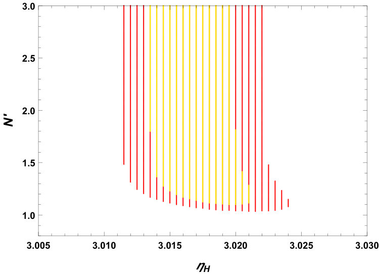 Figure 1
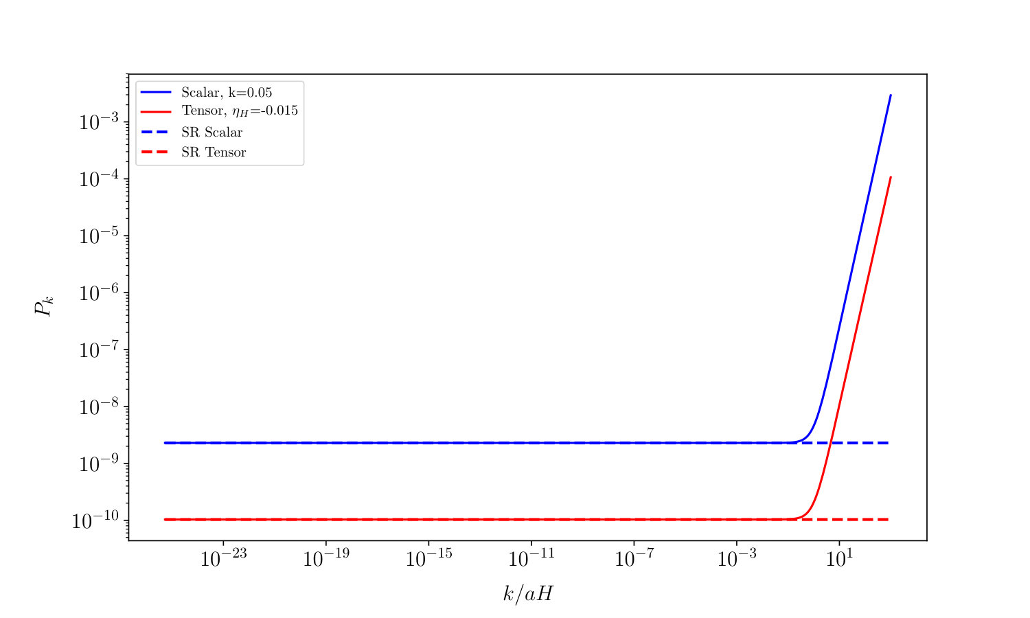 Figure 2
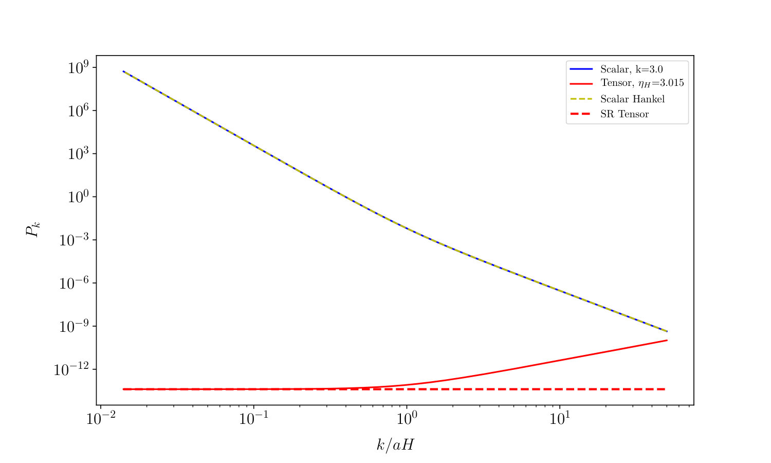 Figure 3
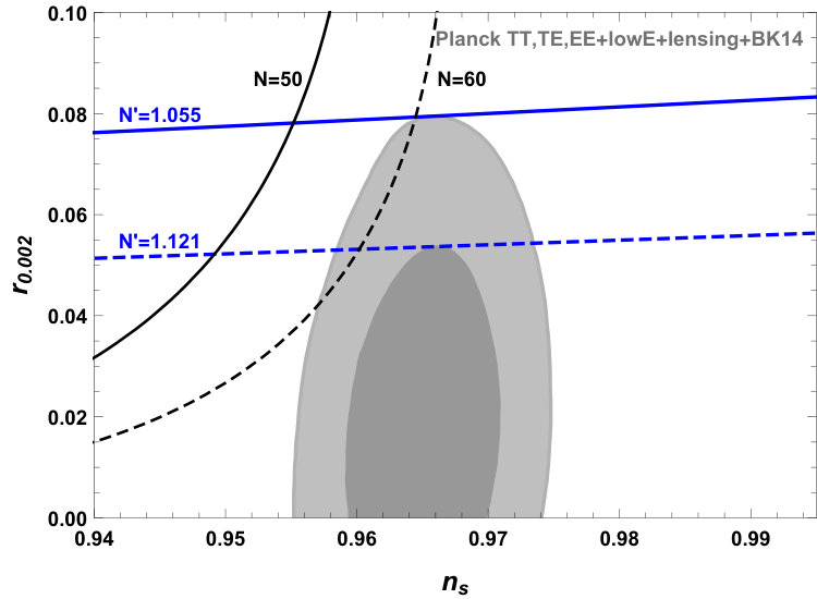 Figure 4
Peer Reviews
No public reviews on file for this paper yet. If you reviewed it on a platform where reviews are public (OpenReview, ICLR, NeurIPS, ICML), you can paste yours below so the community can read it here.
Videos
No videos yet. Explain this paper in a talk, walkthrough, or lecture? Add one.
On the constant-roll inflation with large and small
Qing Gao
School of Physical Science and Technology, Southwest University, Chongqing 400715, China
Yungui Gong
School of Physics, Huazhong University of Science and Technology, Wuhan, Hubei 430074, China
Zhu Yi
School of Physics, Huazhong University of Science and Technology, Wuhan, Hubei 430074, China
Abstract
We study the seemingly duality between large and small for the constant-roll inflation with the second slow-roll parameter being a constant. In the previous studies, only the constant-roll inflationary models with small are found to be consistent with the observations. The seemingly duality suggests that the constant-roll inflationary models with large may be also consistent with the observations. We find that the duality between the constant-roll inflation with large and small does not exist because both the background and scalar perturbation evolutions are very different. By fitting the constant-roll inflationary models to the observations, we get at the 95% C.L if we take for the models with increasing in which inflation ends when , and at the 68% C.L., and at the 95% C.L. for the models with decreasing .
I Introduction
Inflation explains the flatness and horizon problems in standard cosmology, and the quantum fluctuations of the inflaton seed the large scale structure of the Universe and leave imprints on the cosmic microwave background radiation Guth (1981); Linde (1982); Albrecht and Steinhardt (1982); Starobinsky (1980); Guth and Pi (1982). To solve the problems such as the flatness, horizon and monopole problems, the number of -folds remaining before the end of inflation must be large enough and it is usually taken to be due to the uncertainties in reheating physics. This requires the potential of the inflaton to be nearly flat, i.e., the slow-roll inflation. The temperature and polarization measurements on the cosmic microwave background anisotropy conformed the nearly scale invariant power spectra predicted by the slow-roll inflation and gave the constraints (68% C.L.) and (95% C.L.) Akrami et al. (2018); Ade et al. (2018).
Recently, the constant-roll inflation with being a constant Martin et al. (2013); Motohashi et al. (2015) attracted some attentions because the inflationary potential and the background equation of motion can be solved analytically. The slow-roll parameter is a constant and it may not be small, the model is different from the typical slow-roll inflationary models. In particular, when the inflationary potential becomes very flat, , we get the ultra slow-roll inflation Tsamis and Woodard (2004); Kinney (2005). Due to the violation of the slow-roll condition, the curvature perturbation may evolve outside the horizon and the slow-roll results may not be applied Leach and Liddle (2001); Leach et al. (2001); Kinney (2005); Jain et al. (2007); Namjoo et al. (2013); Martin et al. (2013); Motohashi et al. (2015); Yi and Gong (2018). However, for the constant-roll inflation with , the slow-roll parameter decreases with time and is small during inflation, so we can still use the standard method of Bessel function approximation to calculate the power spectra. Neglecting the contribution from , it was found there exists a duality between the ultra slow-roll inflation and the slow-roll inflation Tzirakis and Kinney (2007); Morse and Kinney (2018), i.e., if we replace by , we get the same result for the scalar spectral tilt. Recall that the observational data constrained to be small Motohashi and Starobinsky (2017a); Gao (2018); Galvez Ghersi et al. (2018), these results are in conflict with the duality relation, so it is necessary to revisit the observational constraint to include the constraint on the ultra-slow inflation. For the ultra slow-roll inflation, it is legitimate to neglect . For the typical slow-roll inflation, and are in the same order, so cannot be neglected and it is interesting to discuss the duality up to the first order of in the constant-roll inflation. The difference in may cause different amplitudes for the power spectra or different energy scale of inflation. Furthermore, due to the smallness of in the ultra slow-roll inflation, it can be used to generate a large curvature perturbation at small scales which produces primordial black holes and secondary gravitational waves Germani and Prokopec (2017); Motohashi and Hu (2017); Di and Gong (2018). For more discussion on the constant-roll inflation, please see Refs. Motohashi and Starobinsky (2017b); Oikonomou (2017); Odintsov and Oikonomou (2017); Nojiri et al. (2017); Dimopoulos (2017); Ito and Soda (2018); Karam et al. (2018); Fei et al. (2017); Cicciarella et al. (2018); Anguelova et al. (2018); Gao et al. (2018); Mohammadi and Saaidi (2018); Pattison et al. (2018).
In this paper, we extend the discussion of the duality between the ultra slow-roll inflation and the slow-roll inflation to include the effect of . The paper is organized as follows. In the Sec. II, we review the constant-roll inflation and discuss the duality between the ultra slow-roll inflation with large constant and the slow-roll inflation with small constant . In Sec. III, we fit constant roll models to the observational data. The conclusions are drawn in Sec. IV.
II The constant-roll inflation
We use the Hubble flow slow-roll parameters Liddle et al. (1994),
[TABLE]
where and . In particular, the first three slow-roll parameters are
[TABLE]
[TABLE]
[TABLE]
and the evolution of the slow-roll parameters are
[TABLE]
[TABLE]
where . For the constant-roll inflation with constant , we get . From Eq. (5), we see that if , then increases monotonically with time. Otherwise, if , then decreases monotonically with time. Since , so decreases monotonically with time for the constant-roll inflationary model with , such as the ultra slow-roll inflation with .
The scalar perturbation is governed by Mukhanov-Sasaki equation Mukhanov (1985); Sasaki (1986),
[TABLE]
where
[TABLE]
, is the conformal time, and the mode function for a Fourier mode is related with the curvature perturbation by . To the first order of , , and Eq. (7) becomes
[TABLE]
where
[TABLE]
Since is a constant and the change of can be neglected which is true for both slow-roll and ultra slow-roll inflation 111For the ultra slow-roll inflation, can be very small because it decreases with time., so can be approximated as a constant, the solution to Eq. (9) for the mode function is the Hankel function of order ,
[TABLE]
Therefore, the power spectrum of the scalar perturbation is
[TABLE]
The amplitude of the power spectrum at the horizon crossing is
[TABLE]
The scalar spectral tilt is
[TABLE]
Following the same procedure, we get the power spectrum of the tensor perturbation and the tensor to scalar ratio
[TABLE]
If we neglect the contribution of in Eqs. (10), (14) and (15), we see that these expressions are unchanged if we replace by , i.e., there exists a duality between and as observed in Tzirakis and Kinney (2007); Morse and Kinney (2018). It this duality is true, then we can apply the usual slow-roll results to ultra slow-roll inflationary models. In the previous analysis of the observational constraints on constant-roll inflation, only the model with small was found to be consistent with the observations Motohashi and Starobinsky (2017a); Yi and Gong (2018); Gao (2018); Galvez Ghersi et al. (2018). This duality relation suggests that the ultra slow-roll inflationary models may also be consistent with the observations. To investigate whether this is true, we discuss the issue of duality below.
II.1 The constant-roll models
From Eq. (3), we get
[TABLE]
for . For , the general solution is the form of trigonometric functions and . Following Ref. Motohashi et al. (2015), for we consider the particular solutions
[TABLE]
with the potential ,
[TABLE]
and
[TABLE]
For , the particular solutions are
[TABLE]
and
[TABLE]
For the constant-roll inflation, is known, so is determined from the relation 222For these potentials, solutions other than the constant-roll inflation exist.. We don’t consider the exponential solution because the corresponding power-law inflation is excluded by the observations. The models (18) and (22) were studied in Refs. Motohashi et al. (2015); Motohashi and Starobinsky (2017a); Morse and Kinney (2018); Galvez Ghersi et al. (2018). For the model (18), , so we need to introduce some mechanism to end inflation. The model (20) was studied in Ref. Yi and Gong (2018). As discussed in Ref. Yi and Gong (2018), in the model (20), and , so there is no inflation in this model if , i.e., the model cannot support ultra slow-roll inflation and it is not applicable to the discussion of the duality relation.
II.2 The duality between the slow-roll and the ultra slow-roll inflation
For the slow-roll inflation with and , we get
[TABLE]
[TABLE]
and
[TABLE]
For the ultra slow-roll inflation with and , we get
[TABLE]
[TABLE]
and
[TABLE]
From Eq. (29), we see that to be consistent with the observations , we must take because , so the constant-roll inflation with may be consistent with the observations.
Eqs. (25) and (28) show that the amplitudes of the power spectra for both the slow-roll and ultra slow-roll inflation have the same form. From Eqs. (26) and (29), we see that the power spectra for both the slow-roll and ultra slow-roll inflation are nearly scale invariant. If we neglect in Eqs. (26) and (29), the expressions for the slow-roll inflation with and the ultra slow-roll inflation with are the same, so it seems that there exists a duality between and . In particular, the model (18) is self-dual when . The model (18) with is dual to the model (22) with . Note that for the model (18), while for the model (22). For the model (18) with , the inflaton climbs up instead of rolling down the potential and the constant-roll inflationary solution is not an attractor Motohashi et al. (2015). Furthermore, as shown in Ref. Motohashi et al. (2015), in the model (18) with , the curvature perturbation grows on both the sub-horizon and super-horizon scales, but the curvature perturbation decreases on the sub-horizon scales and is frozen on the super-horizon scales in both the model (18) with and the model (22) as shown in Figs. 1 and 2, so this duality is false because the behaviors of the background and the curvature perturbations are totally different for the constant-roll inflation with large and small . Due to the growth of the curvature perturbations on super-horizon scales for the constant-roll model (18) with , the scalar power spectrum (12) should be evaluated at the end of inflation instead of the horizon crossing Namjoo et al. (2013); Cheng et al. (2016, 2018); Byrnes et al. (2018); Passaglia et al. (2018). For the model (20), because no inflation happens if , so the duality is inapplicable to this model. For the same reason, the model (24) is not dual to the model (20).
Furthermore, is usually not negligible for the slow-roll inflation while it may be negligible for the ultra slow-roll inflation, the amplitudes (25) and (28) for both the scalar and tensor spectra will be different when the effect of is included, so there is no duality in the constant-roll inflation with large and small . In particular, for the ultra slow-roll inflation, the scalar perturbation may be very large and the tensor to scalar ratio may be negligible.
III The observational constraints
For the slow-roll inflation, in terms of the remaining number of e-folds before the end of inflation, from Eq. (5), we get
[TABLE]
where we impose the condition of the end of inflation . This formulae only applies to the model with , like the model (20).
For the ultra slow-roll inflation, decreases monotonically with time and inflation does end, we need some mechanisms to end inflation. Instead of using , we introduce the number of -folds after the start of inflation Galvez Ghersi et al. (2018). From Eq. (5), we get
[TABLE]
where is an integration constant. Take , we get
[TABLE]
Substituting Eq. (31) into Eqs. (14) and (15), we can calculate and for the constant-roll inflation with increasing . Substituting Eq. (33) into Eqs. (14) and (15), we can calculate and for the constant-roll inflation with decreasing . The results along with the Planck 2018 and BICEP2 constraints Akrami et al. (2018); Ade et al. (2018) are shown in Fig. 3. In Fig. 3, the black lines represent the calculated results with Eq. (31) and the blue lines denote the calculated results with Eq. (33). The model with increasing is excluded by the observations if we take (the solid black line) and is marginally consistent with the observations at the 95% level if we take (the dashed black line). The constraint is at the 95% C.L for . The model with decreasing is consistent with the observations, we find that at the 68% C.L. and at the 95% C.L. The constraints on the parameters and for the model (33) are shown in Fig. 4. We get at the 68% C.L., and at the 95% C.L. These results show that there is no duality between and .
IV Conclusions
For the constant roll model (18), and some mechanisms need to be introduced to end the inflation. The scalar perturbation grows on the sub-horizon scales if and the super-horizon scales if . If , the inflaton climbs up the potential and the constant roll solution is not an attractor. For the constant roll model (20), and enough inflation happens only if because in this model.
To the first order of , we derive the formulae for and . If we neglect the contribution of which is a reasonable assumption for the constant roll inflationary models with decreasing during inflation, there exists a duality between small and large with for the expressions of and . Therefore, it seems that the models (18) and (20) are self dual if , the model (18) with is dual to the model (22), the model (20) with is dual to the model (24). As discussed above, there is no inflation in the model (20) with and the behaviors of the background and scalar perturbations for the model (18) with are very different from those in the model (18) with and the model (22), so the seemingly duality between the constant-roll inflation with large and small does not exist. By fitting the constant roll models to the observations, we find that the model with increasing is excluded by the observations if we take . If we take , the constraint is at the 95% C.L. For the models with decreasing , we obtain that at the 68% C.L., and at the 95% C.L. These results confirm that the duality between and does not exist.
Acknowledgements.
This research was supported in part by the National Natural Science Foundation of China under Grant Nos. 11605061 and 11875136, the Major Program of the National Natural Science Foundation of China under Grant No. 11690021, the Fundamental Research Funds for the Central Universities under Grant Nos. XDJK2017C059 and SWU116053. Qing Gao acknowledges the financial support from China Scholarship Council for sponsoring her visit to California Institute of Technology, and thanks California Institute of Technology for the hospitality.
The reference list from the paper itself. Each links out to its DOI / PubMed record.
- 1Guth (1981) A. H. Guth, Phys. Rev. D 23 , 347 (1981) . · doi ↗
- 2Linde (1982) A. D. Linde, Phys. Lett. B 108 , 389 (1982) . · doi ↗
- 3Albrecht and Steinhardt (1982) A. Albrecht and P. J. Steinhardt, Phys. Rev. Lett. 48 , 1220 (1982) . · doi ↗
- 4Starobinsky (1980) A. A. Starobinsky, Phys. Lett. B. 91 , 99 (1980) . · doi ↗
- 5Guth and Pi (1982) A. H. Guth and S. Y. Pi, Phys. Rev. Lett. 49 , 1110 (1982) . · doi ↗
- 6Akrami et al. (2018) Y. Akrami et al. (Planck), “Planck 2018 results. X. Constraints on inflation,” (2018), ar Xiv:1807.06211 [astro-ph.CO] .
- 7Ade et al. (2018) P. A. R. Ade et al. (BICEP 2, Keck Array), “BICEP 2 / Keck Array X: Constraints on Primordial Gravitational Waves using Planck, WMAP, and New BICEP 2/Keck Observations through the 2015 Season,” (2018), ar Xiv:1810.05216 [astro-ph.CO] .
- 8Martin et al. (2013) J. Martin, H. Motohashi, and T. Suyama, Phys. Rev. D 87 , 023514 (2013) , ar Xiv:1211.0083 [astro-ph.CO] . · doi ↗